Chapter 6

Mapping Samples to a Disk

Objectives

By the end of this chapter you should:

• understand the requirements for a good mapping technique from a square to a disk;
• understand how the concentric map is implemented.

We require sample points distributed on a unit disk for the simulation of depth of field with a circular camera lens in Chapter 10 and for shading with disk lights in Chapter 18. As we can already generate samples on a unit square, it’s natural to generate these as before and then map them to a unit disk. Although a number of techniques can be used for this task, some are better than others.

The basic requirement for a good mapping technique is that if the sample points are well-distributed on the unit square, they will also be well-distributed on the disk. In other words, the map should not introduce significant amounts of distortion. As it turns out, this is not trivial to achieve. Another requirement is that the map fits in well with the shading architecture described in the previous chapter.

6.1 Rejection Sampling

Rejection sampling is a technique for generating sample points that satisfy specified geometric conditions. To use rejection sampling to produce samples on a disk, we generate samples on a square that just contains the disk but only keep those samples that are on the disk. Figure 6.1 illustrates this technique with 256 multi-jittered samples.

The best aspect of rejection sampling is that there’s no distortion, but a technical problem is that only a subset of the original samples are kept. This raises the question of what can happen if you only use a subset of a sampling pattern. This question also arose in the previous chapter, but the answer depends on the sampling technique. Although subsets of uniform, random, and jittered pattern are still uniform, random, and jittered patterns, respectively, this does not apply to n-rooks, multi-jittered, or Hammersley sampling. For example, if we used n-rooks to generate the samples on the square, the samples on the disk would not satisfy the n-rooks condition. Although the index shuffling should allow us to avoid serious aliasing problems, it’s far from ideal to have different numbers of samples in different sampler objects. Rejection sampling therefore does not fit in well with my shading architecture.

6.2 The Concentric Map

It’s better to generate the samples on a unit square, where we can specify their exact number and then map all of them to a unit disk. Although there are a couple of simple maps that do this, they significantly distort the samples. The best technique is Shirley’s concentric map, visualized in Figure 6.2, which maps concentric squares to concentric circles and has low distortion. It therefore keeps points that are close together on the square close together on the disk.

We first map the samples to the square [−1, 1]2, where each triangular quarter has to be considered separately. These are the four colored triangles numbered 1–4 in Figure 6.3(a), defined by the lines x = y and x = −y. They are mapped to the corresponding colored sectors of the disk shown in Figure 6.3(b). Although the mapping technique is the same in each quarter, we have to consider these separately because we can’t write the complete map as a single set of equations.

For each quarter of the square, Table 6.1 gives the x and y inequalities defined by the lines x = y and x = −y, the angular range of the corresponding sector, and the map equations.

To implement the map, we add an array disk_samples to the Sampler class to hold the new samples. We also need to add a function map_samples_to_unit_disk to perform the map. This is a member function of the Sampler class because the map is independent of the sampling technique. Listing 6.1 shows the code.

The function map_samples_to_unit_disk is called when we construct an object that has to supply samples on a disk. The object’s set_samplerfunction is the appropriate place to call this. See Listing 10.2 for an example.

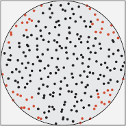
Figure 6.4 shows the samples in Figure 6.1(a) after they have been mapped to the unit disk. The red samples were originally outside the disk.

Finally, the Sampler class requires the function sample_unit_disk, but as this is identical to sample_unit_squareexcept for the name of the samples array, I won’t reproduce the code here. It’s in the file Sampler.cpp on the book’s website. Listing 10.4 shows an example of where this function is called.

void

Sampler::map_samples_to_unit_disk(void) {

     int size = samples.size();

     float r, phi;                                    // polar coordinates

     Point2D sp;                                      // sample point on unit 

     disk

     disk_samples.reserve(size);

     for (int j = 0; j < size; j++) {

           // map sample point to [-1, 1]  [-1,1]

           sp.x = 2.0 * samples[j].x - 1.0;

           sp.y = 2.0 * samples[j].y - 1.0;

           if (sp.x > -sp.y) {                        // sectors 1 and 2

                 if (sp.x > sp.y) {                   // sector 1 

                       r = sp.x;

                       phi = sp.y / sp.x;

                 }

                 else {                               // sector 2

                       r = sp.y;

                       phi = 2 - sp.x / sp.y;

                 }

           }

           else {                                     // sectors 3 and 4

                 if (sp.x < sp.y) {                   // sector 3

                       r = -sp.x;

                       phi = 4 + sp.y / sp.x;

                 }

                 else {                               // sector 4

                       r = -sp.y;

                       if (sp.y != 0.0)               // avoid division by zero 

                       at origin

                             phi = 6 - sp.x / sp.y;

                       else

                             phi = 0.0;

                 }

           }

           phi *= pi / 4.0;

           disk_samples[j].x = r * cos(phi);

           disk_samples[j].y = r * sin(phi);

     }

}

Listing 6.1. The function Sampler::map_samples_to_unit_disk.

Further Reading

The concentric map was developed by Shirley in the early 1990s, but the most accessible reference is Shirley and Chiu (1997). Listing 6.1 is based on code in this reference.

Pharr and Humphreys (2004) also discusses maps from squares to disks. In addition to the concentric map, they discuss two maps that distort the distribution of points. One of these is the polar map $\left(r,\theta \right)=(\sqrt{r_1}, 2\pi r_2)$.

Questions

• 6.1.  It’s simple to generate a specified number of samples on a disk with rejection sampling using one of the sampling techniques discussed in Chapter 5. Which technique is this?
• 6.2.  Suppose we used rejection sampling as in Figure 6.1(a) with n uniformly distributed samples in the square. In the limit n → ∞, what fraction of the samples will be on the disk?

Exercises

• 6.1.  Examine Figure 6.3, Table 6.1, and the code in Listing 6.1 for the concentric map. Make sure you understand the x and y inequalities for each quarter of the square and how the formulae are implemented in the code.