
Chapter 10
Depth of Field

Image courtesy of Tania Humphreys
Objectives
By the end of this chapter, you should:
- understand how depth of field is simulated in ray tracing;
- have implemented a thin-lens camera.
The depth of field of a camera is the range of distances over which objects appear to be in focus on the film. A photographer can set the depth of field of a real camera by adjusting the camera lens. In contrast, everything is in focus with the pinhole camera we modeled in Chapter 9 because the “lens” is infinitely small. Real cameras have finite-aperture lenses that only focus perfectly at a single distance called the focal distance. I’ll present here a virtual camera that simulates depth of field with a finite-radius circular lens.
10.1 Thin-Lens Theory
We first need to cover some classic thin-lens theory from optics. Figure 10.1 shows the cross section of a thin lens composed of two spherical surfaces, and some rays that go through the lens. A magnifying glass is a good model for this.1 Thin-lens theory is an approximation that applies when the thickness of the lens is negligible compared to its radius. In this case, the lens has a number of simple and useful optical properties. Consider a plane that’s perpendicular to the lens axis, for example, the plane labeled the focal plane in Figure 10.1. As there’s nothing special about this, it doesn’t matter where it’s located. A thin lens will focus points on this plane onto another plane on the other side of the lens. This is the image plane in Figure 10.1. Every point p on the focal plane has a corresponding image p′ on the image plane. For an ideal thin lens, every ray from p that hits the lens goes through the point p′. If this lens were in a real camera and the film were on the image plane, the focal plane would be in focus, but everything else would be out of focus to varying degrees.
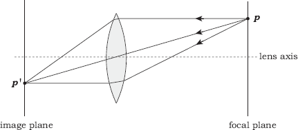
Cross section through a thin lens showing a focal plane and its corresponding image plane.
Each focal plane and image plane exist as a matched pair. They are also interchangeable because light can travel either direction, a fact that I’ll use in Section 10.2. In Figure 10.2, I’ve added a second pair of focal and image planes to the configuration shown in Figure 10.1. The important thing to notice here is that different rays from q hit the image plane of p′ at different places. For rays that only make a small angle with the lens axis, the area they cover is roughly circular and is known as the circle of confusion. If we placed a film on this image plane in Figure 10.2, q would be out of focus. The further q gets from the focal plane of p (on either side), the larger the circle of confusion becomes, and the more out of focus q becomes.

Rays starting a point q go through the image plane of p at different locations, with the result that q will appear out of focus.
The depth of field of a camera is the range of distances parallel to the lens axis in which the scene is in focus. By this definition, a camera made with the above thin lens would have zero depth of field. In contrast, photographs taken with traditional film cameras can appear in focus over finite distances, or off to infinity, because of the finite size of the film grains. In ray tracing and digital cameras, the image can appear in focus over the range of distances where the circle of confusion is smaller than a pixel.
Figures 10.1 and 10.2 also illustrate another property of a thin lens: a ray that goes through the center of the lens is not refracted. I’ll also use this in Section 10.2.
10.2 Simulation
To simulate depth of field, we have to simulate the optical properties of the thin lens discussed above. Although to do this exactly would be a complex process, it turns out that we can make a couple of simplifications and still get convincing results. First, we represent the lens with a disk. Because the disk has zero thickness, we are not quite simulating a real thin lens, which always has finite thickness. The disk is centered on the eye point of the camera and is perpendicular to the view direction, as Figure 10.3 illustrates. Second, we don’t calculate exactly how the light is refracted as it passes through the lens.
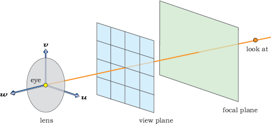
A thin-lens camera consists of a disk for the lens, a view plane (as usual), and a focal plane, all perpendicular to the view direction.
The simulation usually requires a large number of rays per pixel whose origins are distributed over the surface of the lens. We can use the concentric map from Chapter 6 to perform the distribution. Figure 10.4 shows two light paths that join corresponding points on the focal and image planes,2 where one is the straight line through the center of the lens and the other is through a sample point on the lens. For each path, we start a primary ray on the lens.
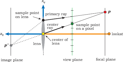
This figure shows two rays projected onto the (xv, zv)-plane. The center ray starts at the center of the lens and hits the focal plane at p. The primary ray starts at a sample point on the lens and also hits the focal plane at p.
The center ray starts at the eye point at the center of the lens and goes through a sample point on a pixel. In common with the pinhole camera, the thin lens camera has the view plane on the opposite side of the lens as the image plane, but this doesn’t invalidate the simulation. The primary ray starts on a sample point on the lens. To simulate depth of field we perform the following three tasks:
- compute the point p where the center ray hits the focal plane;
- use p and the sample point on the lens to compute the direction of the primary ray so that this ray also goes through p;
- ray trace the primary ray into the scene.
There are a couple of things to note about this procedure. First, the center ray doesn’t contribute any color to the pixel; we only use it to find out where p is. It’s the primary rays that form the image. The second thing to notice is that the process does take refraction through the lens into account. The two paths from p′ to p are thin-lens paths for an infinitely thin lens, but we don’t start the rays at p′ and refract them through the lens. Instead, we start the primary rays on the lens but make sure they point in the correct direction.
The above process produces good results, but if we used a single center ray for each pixel, all primary rays for a given pixel would hit the focal plane at the same point p, as Figure 10.5 illustrates. This will result in the focal plane being perfectly in focus but with no antialiasing.

If all of the primary rays for a given pixel hit the focal plane at the same point, it will be in perfect focus but will not be antialiased.
Although the blurring effects of depth of field can obliterate aliasing artifacts as hit points move away from the focal plane, it’s still best to use antialiasing, because this improves the appearance of the scene that’s near the focal plane. We can easily accomplish this by using a different center ray for each primary ray. See Figure 10.6, where four center rays go through different sample points on the pixel and therefore hit the focal plane at different locations.

Figure 10.7 shows four primary rays that start at sample points on the lens and hit the focal plane at the four points shown in Figure 10.6. Notice that the top ray does not go through the pixel that’s being sampled, but that’s all right because there’s no geometric requirement for that to happen with thin-lens primary rays.

Four primary rays that start at sample points on the lens and hit the focal plane at the same points that the center rays in Figure 10.6 hit it.
This technique fits in well with the sampling architecture from Chapter 5, where for each pixel, we use the same number of samples for antialiasing and sampling the lens. We can also use different sampling techniques for each, if we want to.
We don’t have to trace the center rays to find out where they hit the focal plane. Instead, we can use similar triangles as indicated in Figure 10.8. This is a projection of the rays and points onto the (xv, zv) plane, where the three relevant points are a pixel sample point ps on the view plane, a sample point ls on the lens, and the point p on the focal plane. The viewing coordinates of these points are
p=(px,py,-f),ps=(psx,psy,-d),ls=(lsx,lsy,0),
where f is the focal length of the camera, because this is the distance along the view direction that’s in focus, and d is the view-plane distance. These will be user-specified parameters for the thin-lens camera described in Section 10.3.

The x- and y-components of ps are known quantities, given by Equations (9.4). The x- and y-components of ls are also known because the sampler object stored in the thin-lens camera returns a sample point on a unit disk, and the x- and y-components are then multiplied by the lens radius (see Listing 10.4). It follows from similar triangles that
px=psx(f/d) (10.1)
and
py=psy(f/d). (10.2)
The direction of the primary ray is then
dr=p-ls=(px-lsx)u+(py-lsy)v-fw. (10.3)
As this is not a unit direction, you will have to normalize it before tracing the ray.
10.3 Implementation
The ThinLens camera class is declared in Listing 10.1. Although this has a number of new data members, we don’t need to store the number of lens samples because these are accessed in lockstep with the pixel samples.
class ThinLens: public Camera {
public:
// constructors, access functions, etc
void
set_sampler(Sampler* sp);
Vector3D
ray_direction(const Point2D& pixel_point, const Point2D&
lens_point) const;
virtual void
render_scene(World& w);
private:
float lens_radius; // lens radius
float d; // view plane distance
float f; // focal plane distance
float zoom; // zoom factor
Sampler* sampler_ptr; // sampler object
};
Listing 10.1. Declaration of the class ThinLens
void
ThinLens::set_sampler(Sampler* sp) {
if (sampler_ptr) {
delete sampler_ptr;
sampler_ptr = NULL;
}
sampler_ptr = sp;
sampler_ptr->map_samples_to_unit_disk();
}
Listing 10.2. The function ThinLens::set_sampler.
Vector3D
ThinLens::ray_direction(const Point2D& pixel_point, const Point2D& lens_point)
const {
Point2D p; // hit point on focal plane
p.x = pixel_point.x * f / d;
p.y = pixel_point.y * f / d;
Vector3D dir = (p.x - lens_point.x) * u + (p.y - lens_point.y) * v - f * w;
dir.normalize();
return (dir);
}
Listing 10.3. The function ThinLens::ray_direction.
In contrast to the function ViewPlane::set_sampler in Listing 5.3, the ThinLens::set_sampler function in Listing 10.2 doesn’t use regular sampling when the number of samples per pixel is one. Instead, their distribution will be determined by the type of sampling object used. The ray origins will be randomly distributed over the surface of the lens when we use random, jittered, and multi-jittered sampling. As a result, the images will become progressively noisier as the lens radius increases. This will, however, quickly show you the depth-of-field effects. See Figure 10.9(b) for an example. Note that ThinLens::set_sampler also maps the sample points to the unit disk.

(a) When the lens radius is zero, the image is the same as a pinhole-camera image with everything in focus; (b) noisy image from using one random sample per pixel.
The function ray_direction in Listing 10.3 follows directly from Equations (10.1)–(10.3).
Finally, the ThinLens::render_scene function in Listing 10.4 illustrates how the pixel and lens sampling work together.
10.4 Results
Listing 10.5 shows part of the build function for the following images. Notice that the pixel size is 0.05, which is much smaller than the default value of 1.0. This is so that we use a view-plane distance (40) that’s less than the focal distances used in the images below. All this does, however, is make the camera configuration consistent with the figures in Section 10.2. You need to look at Questions 10.1 and 10.2 and do Exercise 10.2.
Figures 10.9 and 10.10 show three boxes and a plane with checker textures. Figure 10.9(a) shows the scene with everything in focus by using a lens radius of zero. Figure 10.9(b) shows the noisy type of image that results from using a single multi-jittered sample per pixel and a lens radius of one. Here, the front face of the far box is on the focal plane and is therefore in focus.
void
ThinLens::render_scene(World& w) {
RGBColor L;
Ray ray;
ViewPlane vp(w.vp);
int depth = 0;
Point2D sp; // sample point in [0, 1] X [0, 1]
Point2D pp; // sample point on a pixel
Point2D dp; // sample point on unit disk
Point2D lp; // sample point on lens
w.open_window(vp.hres, vp.vres);
vp.s /= zoom;
for (int r = 0; r < vp.vres - 1; r++) // up
for (int c = 0; c < vp.hres - 1; c++) { // across
L = black;
for (int n = 0; n < vp.num_samples; n++) {
sp = vp.sampler_ptr->sample_unit_square();
pp.x = vp.s * (c - vp.hres / 2.0 + sp.x);
pp.y = vp.s * (r - vp.vres / 2.0 + sp.y);
dp = sampler_ptr->sample_unit_disk();
lp = dp * lens_radius;
ray.o = eye + lp.x * u + lp.y * v;
ray.d = ray_direction(pp, lp);
L += w.tracer_ptr->trace_ray(ray, depth);
}
L /= vp.num_samples;
L *= exposure_time;
w.display_pixel(r, c, L);
}
}
Listing 10.4. The function ThinLens::render_scene.
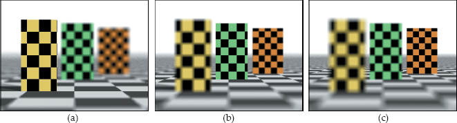
Each of these images shows the camera focused on the front face of one of the boxes, where the view plane distance is 40 and the focal distance is 50 (a), 74 (b), and 98 (c).
Figure 10.10 shows the scene where the camera is focused on the front face of each of the three blocks in turn. Notice how your attention is drawn to the block that’s in focus. These images were rendered with a lens size of 1.0. Although the 100 samples per pixel used here is adequate for most parts of these images, there’s still noise near the horizon.
void
World::build(void) {
int num_samples = 100;
vp.set_hres(400);
vp.set_vres(300);
vp.set_pixel_size(0.05);
vp.set_sampler(new MultiJittered(num_samples));
vp.set_max_depth(0);
tracer_ptr = new RayCast(this); // see Section 14.5
background_color = white;
Ambient* ambient_ptr = new Ambient;
ambient_ptr->scale_radiance(0.5);
set_ambient_light(ambient_ptr);
ThinLens* thin_lens_ptr = new ThinLens;
thin_lens_ptr->set_sampler(new MultiJittered(num_samples));
thin_lens_ptr->set_eye(0, 6, 50);
thin_lens_ptr->set_lookat(0, 6, 0);
thin_lens_ptr->set_view_distance(40.0);
thin_lens_ptr->set_focal_distance(74.0);
thin_lens_ptr->set_lens_radius(1.0);
thin_lens_ptr->compute_uvw();
set_camera(thin_lens_ptr);
...
}
Listing 10.5. Part of a build function that demonstrates how to construct a thin-lens camera.
As the lens size increases, the amount of blurriness in the images increases because the radius of the circle of confusion at a given distance from the focal plane is proportional to the lens radius. The effective depth of field also decreases because the radius of confusion becomes larger than a pixel at a smaller distance from the focal plane. These effects are demonstrated in Figure 10.11(a), which is the same as Figure 10.10(c) but rendered with a lens radius of 3.0. To keep noise to an acceptable level, we usually need to use more samples per pixel as the radius increases.

(a) As the lens radius increases, the image becomes more out of focus, the depth of field decreases, and we require more samples per pixel. This image was also rendered with 100 samples per pixel and is quite noisy; (b) a large value for the focal distance results in the whole image being out of focus except the horizon.
In Figure 10.11(b), the focal distance is 100000, which is essentially infinity, and as a result, the horizon is the only part of the scene in focus. In this image, the lens diameter is 0.25.
Further Reading
As thin-lens theory is a part of classic geometric optics, most optics textbooks discuss it. See, for example, Hecht (1997).
The landmark paper by Cook et al. (1984) was the first paper to simulate depth of field in ray tracing. This paper also introduced motion blur, soft shadows, glossy reflection, and glossy transmission!
Kolb et al. (1995) used a physically based camera model with a finiteaperture, multi-element thick lens for ray tracing. This is a much more sophisticated camera model than the one discussed here.
Questions
- 10.1. Is the simulation in Section 10.2 still applicable when the view plane is farther from the lens than the focal plane?
- 10.2. How do you zoom with a thin-lens camera?
- 10.3. Figure 10.12 shows a thin box with a mirror material, sitting on a ground plane. The focal plane, which I’ve added to the scene and rendered in red to make it visible, cuts the ground plane behind the box. The part of the plane that’s reflected in the box is therefore not only in front of the focal plane but is actually farther away from it than the box . Why, then, is part of the reflected plane in focus?

- 10.4. Figure 10.13 is the same as Figure 10.9(b), except that it’s rendered with one regular sample per pixel. Can you explain the result?

Exercises
- 10.1. Implement a thin-lens camera as described here and test it with the images in Section 10.4.
- 10.2. Experiment with different values for the view-plane distance, focal distance, lens radius, and number of samples per pixel. In particular, render some images when the view-plane distance is larger than the focal distance.
- 10.3. Experiment with different sampling patterns on the lens, including Hammersley sampling.
1. After reading Chapters 19 and 27, you should be able to model and render a magnifying glass.
2. In this and other 2D figures, I’ve drawn the lens with a finite thickness to make it visible.