CHAPTER 20

Studio Monitoring Systems

Ideally, the main control room monitoring system in any studio should be of high resolution, full audio bandwidth, low distortion and should be able to provide sufficient sound pressure level at the mixing position for all forms of music recording likely to be undertaken in the studio. As discussed in the previous chapter, there are people, some of them with great skill, flair and experience, who choose to work principally on their favourite mid or small sized monitor loudspeakers, but that does not negate the need for a high-quality system. If they choose not to use the large monitors, then it is their prerogative to do so. Nevertheless, it should be incumbent on all professional studios to have available a full range monitor system for persons who wish either to work on them as standard practice, or to use them to check for things which are outside of the range of performance of the small monitors.

Although studio monitor system design is a huge subject, well beyond the scope of this book (see Bibliography), this chapter discusses many of the aspects of the component parts of a monitor system which need to be taken into consideration, both in terms of the functionality of the entire control room, and the way that they may influence overall results. For example, the characteristics of a cabinet which influence the way that it needs to be mounted, or the effects of loudspeaker cables which may dictate the siting of the amplifiers. It needs to be well understood that loudspeaker systems are not self-contained, independent entities which can simply be wheeled into a control room and be expected to be ready for use as soon as the acoustic construction has been completed. In fact, there are several aspects of studio monitor design that cannot be considered independently of the control room design as a whole.

20.1 The Constituents of the System

The monitor chain really begins in the monitor circuitry of the mixing console, because everything heard in the control room will pass through the console’s monitor level control. The circuits which feed that control, the input selector circuits, are therefore the true front end of the monitor system. From the mixing console we then need audio cables to the inputs of the crossover if the loudspeaker system is active or to the amplifiers if the system is passive.

In the former case we would then pass to the amplifiers and on to the loudspeaker drive units via suitable loudspeaker cables. In the latter case, the amplifiers would connect to the high-level crossover via suitable loudspeaker cable, and thence to the loudspeaker drive units. The drive units (drivers) will be mounted in some form of enclosure, which will modify their free-air response, and from the cabinet mounted drivers the air in the room will couple the loudspeaker vibrations to the ears, via any obstructions that they may find in their way. This entire pathway describes a studio monitor system.

In a monitor system there are therefore many different component parts, and not only the parts themselves determine the overall system response. The interfacing must also be considered, because interactions can take place between inputs and outputs which must be carefully and suitably matched if response disturbances are not to result in signal degradation. The interfacing cables can also be sources of interference and general signal degradation if not chosen appropriately, although the better professional equipment tends to be much more tolerant of cabling than a lot of the domestic hi-fi equipment due to the generally more robust circuits in the input and output stages. Nevertheless, care still needs to be exercised when selecting appropriate cabling.

Let us therefore consider the needs and pitfalls as a signal passes from the output busses of a mixing console on its way to the ears of the recording personnel. In this way, we can discuss the options available and any problems as they arise. The description of the monitor system in the previous couple of paragraphs seems simple enough, but the realities are somewhat more complicated. Inevitably, this will be a chapter of some considerable length, because the options and dilemmas are multifarious.

20.2 Console Monitor Circuitry

On completion of a control room it is customary for studio designers to play a range of recordings which are well known to them in order to confirm, aurally, that all is performing according to expectation. As mentioned in Chapter 18, the introduction of a mixing console into a room can cause considerable acoustic disturbance, which in the past has often been confused with a change in sound due to the mixing console electronics. Nevertheless, the monitor circuitry of many consoles leaves much to be desired, and so there are two ways that a mixing console can degrade the monitoring performance of a control room: acoustically and electrically.

The classic test for mixing console electronic transparency is to connect a signal source directly to the power amplifiers in the case of a passive loudspeaker system or to the input of the electronic crossover if the system is multi-amplified. In either case, care should be taken to ensure that the signal source (CD or DVD player, for example) has outputs that are suitable for driving the crossover or amplifier inputs correctly. The next stage is to listen carefully to a selection of recordings, and then listen again with the signal source connected via the ‘tape returns’ of the console monitor circuitry. If any difference is heard in the signal clarity, stereo width, transparency, stereo imaging, frequency response or any other aspect of the sound quality, then one should begin to worry about the console monitor circuitry. All too often, a difference is heard, and in some cases it is not a subtle difference. Many very expensive mixing consoles are not immune to this problem. It should be noted that such tests can only be truly meaningful if the signal source is of very high quality. If, for example, a cheap CD player is used, it may itself limit the reproduction quality to such a degree that the lesser degradation due to the console would not be evident, so any D to A converters used in these tests should also be of the highest quality.

There seems to be a tendency amongst many mixing console manufacturers to cut costs in the monitor circuits, in the misguided belief that as they are not in the direct signal path of the recording they are somehow less important than the mixing busses in terms of minimising noise and maximising quality. Of course the mixing bus outputs are of great importance, because the final programme will pass through them, but unless the monitor circuitry is of equal quality, or better, then one has no way of knowing the precise quality of what is being recorded.

Some mixing consoles of reputable manufacture have been shown to be seriously lacking in terms of monitor circuit quality. Sometimes as little as an extra €6 or €7 per stereo monitor channel could significantly increase the quality of the sound that passes through them. Unfortunately, the competition between the manufacturers is so fierce that the cost of improvement to six stereo monitor inputs (mix out, tape returns, etc.), which could add €100 to the price of a console, is a cost which they would rather avoid. Believe it or not, consoles costing €100,000 or more have been subject to such miserly cost cutting. This seems totally disgraceful, but it is a reality of the de-professionalisation of the music recording industry. Even studios that are trying hard to be professional are often subject to performance degradation due to hidden cost cutting of a nature such as described above.

In fact, one reason why manufacturers have got away with such shoddy practices is because many of the monitor systems used in current studios are of too poor quality to reveal the problems. It has been demonstrated clearly in studios with excellent monitoring that differences that can be plain for all to hear can be rendered totally inaudible on loudspeakers such as NS10s. This must not, however, be taken as a criticism of the NS10s, per se, because they were never intended to be used as the principle quality references. Their value has been in achieving appropriate musical balances, and on certain styles of music they have shown themselves to be useful tools for such work. However, it does emphasise once again the need for high resolution monitoring in a professional studio, irrespective of whether they are going to be generally used for mixing, or not.

Clearly, it is what is on the main mixing busses which goes to the recording medium, but all the decisions about the correctness or suitability of the sound will be made via a monitor system which begins with the pick up of the monitor signal from those mixing busses. The dials and gauges on a racing car do not directly affect the performance of the car, but they do influence its performance via the information which they feed to the driver. Monitoring is somewhat similar, the ultimate performance of a mix or a recording is affected by the information that the monitors feed to the musicians and recording personnel during the recording or mixing process.

Sometimes, it must be said, the lack of attention to detail in the monitor circuits of quite expensive mixing consoles can be disgraceful. Flimsy printed circuit tracks that are badly screened and of very unequal length, in what may be ostensibly balanced circuits, are often typically to be found. The ‘balanced’ circuitry is also often found to be designed around single op-amps, which cannot be used to derive truly balanced inputs. The consoles also often fail to come with adequate explanations about the circuit topologies or the recommended way of unbalancing them if it is necessary to do so; for example, whether the negative (cold) connections of the inputs or outputs should be grounded or left floating. This is relevant because not all amplifiers in studio use have balanced inputs. Inappropriate connection can be infuriatingly difficult to trace, because often no normal test equipment will show any obvious fault condition or response anomalies. However, correct termination can transform the monitoring clarity. Monitoring systems do need to be considered as single systems, and not a sum of individual parts, but what goes on inside a mixing console monitor section is rarely within the control of a studio designer. In fact, investigation and improvement is often actively discouraged by studio owners, who fear that the guarantees (warranties) may be rendered void if their brand new mixing console is modified. Manufacturers are often reluctant to make modifications at a studio’s request because it first necessitates admission that all is not as good as it could be with the stock item.

It really cannot be over-emphasised that one can no longer presume that high-quality mixing consoles have been built with the highest fidelity in mind. More often, they tend to be built for the maximisation of the characteristics for which they are individually best known, and to meet the points on the price-versus-performance curves which their marketing departments consider most profitable. Even consoles costing over €500,000 are not immune to political interference in their design. Therefore, it is down to the studio owners and users themselves to make sure that the monitor circuitry is not limiting the performance of the entire monitoring chain, and to take whatever action they deem to be appropriate if it is found to be doing so. As previously mentioned, a high-resolution monitoring system and high-quality sound sources (very high-quality D to A converters, also) will be needed for any tests, or the failings may go unnoticed, as they so often do in daily use.

20.3 Audio Cables and Connectors

In general, the higher quality mixing consoles have well-designed balanced outputs; and most professional monitor amplifiers and electronic crossovers have well-designed balanced inputs. They are usually very tolerant of the type of cable that is used to interconnect them. Nevertheless it is good engineering practice to keep cable runs to a minimum between the console outputs and the crossover or amplifier inputs, and to avoid running the cables in parallel with other cables such as data cables or power cables which may be likely to induce interference into the monitor signals.

It tends to be the case that many less expensive consoles, with less advanced output circuitry, are more sensitive to the type of cable used to feed the main monitor system. Perversely, the more money that is spent on the mixing console usually means that less money needs to be spent on the cable. Although good quality cable should always be used, esoteric cables have often been shown to exhibit little sonic benefit when used with high-quality consoles. It should be remembered that professional audio systems interface at 10 to 20 dB higher levels than domestic equipment, precisely to reduce the effects of interference. Together with the lower impedances of the inputs and outputs, this helps to make interfacing much less critical than can be the case with domestic hi-fi.

There are those who argue that the reason why no difference is usually noticeable between good quality and esoteric monitor interface cables is that one is merely adding a few metres to a monitor circuit, when the mixing console itself may contain dozens of metres of ‘normal’ cable from the monitor modules to the jackfield (patchbay) and to the output connectors. Hundreds and even thousands of metres of cable can be used in some large consoles. Some studios have been known to re-wire entire consoles with oxygen-free signal cable, and improvements in sound quality have been claimed, but few opportunities exist to compare directly the modified and unmodified consoles under the same, controlled conditions. In any case, the sheer quantity of cable within the console is likely to swamp the benefits of esoteric cables connecting the console to the main monitors. In the case of cables feeding the close-field monitors, they are most likely to be too short for subtle cable differences to show much effect due to the low impedance balanced circuitry typical of most good monitor systems. However, there is some evidence to suggest that the cable quality becomes more critical as it handles more signals that are complex, so the monitor interface cables could be more critical than those connecting a single channel module, but this is difficult to prove.

As with the cables, good quality connectors should also be used, but there is little to suggest that any significant benefits result from the use of special connectors. Good quality, well-made soldered joints are an obvious requirement.

20.4 Monitor Amplifiers

There can be no doubt that power amplifiers can sound noticeably different to one another. However, what cannot be said is that there is any absolute order of quality. Clearly, a poor amplifier will surely always be worse than a good one, but amongst good ones, things can become very dependent upon circumstances. A well-documented test took place at the Tannoy factory in Scotland in the early 1990s.¹ Intending to recommend a standard amplifier with a new range of four loudspeakers, they had difficulties in making a choice. Eventually they opted to ask some respected persons to carry out blind testing. Four amplifiers were chosen for the comparisons. What had been expected was that one amplifier would be chosen as being superior to the others by the ‘golden ears’, but the reality was very different. In repeatable tests, one of the amplifiers was chosen to be the best on two of the loudspeakers, one on another and a third amplifier on the remaining loudspeaker. Only one of the amplifiers was not chosen to be the best on any of the four loudspeakers.

Loudspeakers present an enormous range of different load conditions to the amplifier outputs, and amplifier performance can be influenced by the loading to a considerable degree. Loudspeakers with high level, passive crossovers vary enormously in the terminations that they present to the amplifiers. Some loudspeakers (principally for hi-fi use) have impedance corrected crossovers and can present an almost perfect 8 Ω load to the amplifier. At the other extreme, monitor loudspeakers such as the Kinoshitas have nominally 4 Ω impedances, but can drop to as low as 0.8 Ω at certain frequencies and under certain drive conditions. Given their enormous power handling of around 1000 W, under certain drive conditions the Kinoshitas can call for as much as 100A from the power amplifiers. This is way in excess of what many power amplifiers can deliver, even if they are rated at 1000 W into 4 Ω, which according to the specifications alone should be sufficient to drive the Kinoshitas (shown in Figure 20.1). The simple I²R formula cannot be applied to difficult loads, because reactive currents can be enormously underestimated. In the above case, it would suggest:

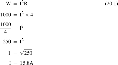
less than 16% of the true peak current demand.

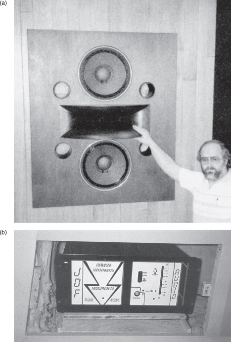
Figure 20.1:

Kinoshita ‘28 Hz’ monitor at Masterfonics, Nashville, USA, and a typical amplifier. (a) The vertical ‘D’Appolito’ mounting configuration gives rise to much less response change with position when moving around in a control room. The concept allows the simplicity of a two-way system to be a practical solution for large monitors, as well as small ones; (b) A JDF amplifier, of enormous output current capacity, of a type often used with the Kinoshita monitors.

Loudspeaker sensitivities also vary widely. Two studio monitors commonly in use in the 1990s were the large, 3 × 15 inch+horn UREI 815, and the small ATC SCM10. The sensitivity of the UREI is 103 dB at 1m distance for 1 W (more accurately 2.83 V) input. The sensitivity of the SCM10 is 81 dB at 1 m for 1 W input. The effect of the sensitivity difference is that in order to sound as loud as a 1 W input into the UREI, the SCM10 would need 158 W, which is +22 dB relative to 1 W. If both loudspeakers were to be driven by a 100 W amplifier with the intention of listening at a sound pressure level of 90 dB SPL at 2 m (equivalent to 96 dB at 1 m in free-field conditions), which is quite a reasonable monitoring level, then very different demands would be made from the amplifier. In the case of the UREI, the typical power demand from the amplifier would be less than a quarter of a watt. (1 W would produce 103 dB at 1 m, hence 6 dB less at 2 m.) For the same SPL, the ATC would need to take 32 W from the amplifier.

Amplifier distortion figures are usually quoted in relation to maximum output power prior to the onset of gross distortion. Their performance at very low output power is rarely specified, but it can have a great bearing on their sound quality under different circumstances. In the case of the ATC loudspeaker in the previous paragraph, signals 20 dB below the normal level would, during quiet passages for example, need just over a quarter of a watt. The UREI, producing a similar SPL would require only just over 2 milliwatts. The performance of different 100 W amplifiers at the 2 milliwatt level can be very different indeed. At such levels, crossover distortion in particular can become a very significant proportion of the output, and can produce rather nasty audible effects. When one considers some mid-range horn loudspeakers with sensitivities in the order of 110 dB at 1 m for 1 W, then the power requirements can be surprisingly low. When playing quieter passages of music, 20 dB below a 90 dB normal listening level at 2 m from the source, which is a perfectly reasonable situation in a studio, the power needed would be only 400 microwatts. This represents only 0.4 milliwatts. When serious listening is taking place whilst drawing only microwatts from the amplifier, Class A amplification, which is free from crossover distortion, would seem to be a wise choice, although it must be said that there are other amplifier classes which are also free from crossover (i.e. zero-crossing) distortion these days (see Bibliography – Self [2009]). It is doubtless that many high efficiency mid-range horn loudspeakers have been judged to sound harsh and distorted merely because they are reproducing distortion which their drive amplifiers exhibit at very low levels.

One very great advantage of the multi-way amplification of monitor systems is that amplifiers can be matched much more accurately and appropriately to the individual loudspeakers. The lack of crossover components between the amplifier and the loudspeaker voice coil also gives the amplifier much more authority over the movement of the diaphragm. Nevertheless, a loudspeaker drive unit is still a reactive device (see Glossary), even without passive crossover components, so simple resistive loading of the amplifier is still not achievable. However, a drive unit alone provides a much more comfortable termination to the amplifier than when fed via a high-level passive crossover. Although the aforementioned constant impedance crossover networks also provide an easier load for the amplifier to deal with, they have often been rejected on subjective listening. What is more, at very high power levels, they can become very difficult and expensive to realise. They can also dissipate considerable power in their compensation resistors, and the drawbacks can soon outweigh the advantages.

For the highest quality of monitoring systems it is better to consider the amplifiers carefully in terms of the power requirements, the distortion content at relevant power levels and their ability to drive the required loads. It is usually of little use selecting a ‘favourite’ amplifier from some other set of circumstances and then specifying it in untested circumstances. The results are likely to be less favourable than from the use of a carefully chosen amplifier for the specific purpose.

Another matter for consideration when selecting amplifiers for studio use is mechanical noise. It is now generally considered wise to mount the amplifiers as physically close as possible to the loudspeakers, in order to reduce loudspeaker cable length to a minimum. The mounting of noisy, fan-cooled amplifiers in remote racks is no longer accepted as good engineering practice. The reasons why will be dealt with in the following section. The use of quiet amplifiers, without cooling fan noise or mechanical transformer buzzes, is desirable, unless they are mounted in ventilated enclosures behind flush mounted loudspeakers. Noisy, fan-cooled amplifiers inside a control room are an absurdity, as they add to background noise levels and hence reduce the dynamic range of the monitoring chain of which they form a part. Figure 20.2 shows convection cooled amplifiers mounted below the loudspeakers in a position where loudspeaker cables can be kept to 2 m, or less, and where the clip and protection lights are clearly visible. The openings above and below the amplifiers allow an ample supply of air to circulate through the heat sinks. The cavity behind is highly acoustically damped, to prevent any resonance problems colouring the monitoring.

The close coupling of the amplifiers to the loudspeakers reduces cable impedance effects and allows better damping of loudspeaker resonances. One often sees damping factor figures of 500 or more in the specifications war amongst amplifier manufacturers, but this figure alone is rather meaningless. The damping factor is the ratio of the load impedance to the amplifier output impedance. Amplifiers can actually be made with zero output impedance, which would theoretically give an infinite damping factor, but in practice they may damp the loudspeaker no more than any other amplifier. This is because the loudspeaker cable has resistance, inductance and capacitance, which lumped together form an impedance to the signal flow. This forms part of the amplifier output impedance from the point of view of the loudspeaker. Even 0.1 Ω of loop impedance in the cable feeding an 8 Ω loudspeaker, connected to an amplifier with infinite damping, would result in an effective damping factor of no more than 8 ÷ 0.1 (or, in other words, 80). There is little to suggest that damping factors greater than 40 or 50 are directly audibly beneficial in themselves. For rapid transient response, a high instantaneous output current and a fast slew rate (the ability to make rapid voltage changes – normally measured in volts per microsecond) tend to have more influence on the sound quality than very high damping factors. When judging amplifiers it is essential to avoid the type of false syllogism which goes, ‘Cats have tails, my Rottweiler has a tail; therefore my Rottweiler is a cat’. Unfortunately, such conclusions are drawn on a daily basis. An amplifier’s performance must be considered in its place as a part of a monitor system. It must be understood that no one amplifier is the best in all circumstances.

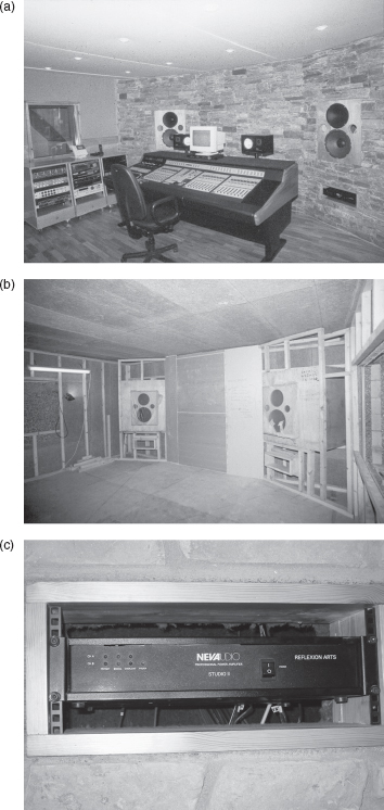
Figure 20.2:

Sonobox, Madrid, Spain. The amplifiers can be seen mounted below the loudspeakers, to ensure the shortest practical cable lengths: (a) The finished control room (2001); (b) loudspeaker and amplifier mounting during construction; (c) The cavity behind the amplifiers must be very well damped to avoid any resonant effects.

Valve (tube) amplifiers, which many music lovers value for home listening, are not usually advisable in recording studio monitor systems. The ‘nice sound’ that they can impart to the music is something that they add to a recording, and therefore the recording itself does not necessarily sound so nice without the help of the amplifier. The principal objective of monitoring is to assess what is on the recording medium, which needs transparent and neutral amplification. When recordings are good, the sound should be good; when recordings are bad, the sound should be bad. At home, when listening for pleasure, one does not really want to hear how bad a recording may be, so valve amplifiers may well be valid, but in the studio it is essential to know when one has a bad sound.

The question of the amplifiers used in ‘active’ monitors, i.e. loudspeakers with built-in amplifiers and electronic crossovers, is something of a two-edged sword. It can cut both ways. Certainly, in an integrated system the manufacturers are in control of everything. There is no loudspeaker cable problem to consider, and the whole electronics package can be designed to provide the correct acoustic response in front of the loudspeaker. In fact, it is the case with many small loudspeakers that their extended response and high output SPLs are only achievable by using dedicated electronics packages with in-built response correction and overload protection. The distortion produced during low frequency overloads in a passively crossed over system tends to send much of the distortion products into the tweeters, resulting in harsh sounds and the need for the frequent replacement of blown diaphragms or coils. By means of the use of separate amplifiers, distortion products are constrained within the bands that produce them, and therefore cannot affect components in other frequency bands.

The negative aspect of the built-in amplifiers is that in today’s marketing driven industry they have probably been built to a ‘just good enough’ quality. The user cannot upgrade the amplification system if he or she decides to spend more on the electronics than the manufacturer has allocated to them. It is an unfortunate but absolute fact that almost all such monitors are built with a competitive price higher in the order of design priorities than the absolute sound quality.

20.5 Loudspeaker Cables

The number one ‘golden rule’ about loudspeaker cables is, ‘the shorter the better’. An enormous amount of pseudo-science clouds this subject, but a few simple facts can be clearly stated. All cables exhibit a mixture of resistance, inductance and capacitance. Resistance is a bad thing, and should be minimised. It wastes power, reduces the ability of the amplifier to control the low frequency cone movement, and forms a potential divider with both the amplifier output impedance and the loudspeaker input impedance. In the former case, it affects the control of back-e.m.f.’s (see Glossary) and in the latter it can cause modification of timbre if the crossover and/or drive units have non-uniform impedance/frequency characteristics.

Inductance is also a bad thing. Its effect is frequency dependent, and series inductance will act as a low pass filter, gradually attenuating high frequencies. Inductance can also be a means of contamination by radio frequency interference, which can enter the amplifier via the loudspeaker cables and cause grittiness in the sound. Low cable inductance is essential for high-quality monitoring systems. Capacitance, however, is rather innocuous. It can, if rather large, cause instability in some amplifiers, but such instability is usually seen to be more a shortfall of the amplifiers’ ability to tolerate capacitive loads rather than being a problem due to the cable capacitance itself. Hence, if cable construction can trade inductance for capacitance, in general the lower inductance option would be preferable.

The negative effects of loudspeaker cable are exacerbated by length, and by the width of the frequency range that they are handling. Long cables from a remote amplifier room to full-range (passively crossed over) loudspeakers are a worst case. In some cases where 5–10 m of cable is run to a loudspeaker with an internal passive crossover, cables of special construction costing typically €2500 each are known to be in use. Moving the crossover away from the loudspeaker and close to the amplifier can help matters. By running separate cables from the crossover to the low frequency and high frequency drive units, the length of cable that handles the full frequency bandwidth can be restricted to the short section from the amplifier to the crossover. It also takes the crossover away from any magnetically hostile loudspeakers. Little will be improved in terms of low frequency damping, but the higher frequencies can be rendered more transparent.

The low frequency currents can often exceed the high frequency currents by thousands of times. Under such circumstances, magnetostriction effects, the attraction and repulsion between the individual cables in a pair, and the dielectric charge migration may, in high power systems, superimpose artefacts of the enormously greater low frequency currents on the high frequency signals in cables carrying full frequency band signals. By separation of the cables to the low and high frequency drivers, such superimposition can be greatly reduced. Another, more usual variation on this bi-wiring theme is where the crossover remains in the loudspeaker cabinet but the common inputs to the high and low pass sections are separated. Individual cable pairs are then run from the high frequency and low frequency filter inputs, back to the amplifier. However, the advantage of removing the crossover from the proximity of the loudspeaker drive units is that the possibility of magnetic induction effects, which can interact between the motor systems and the crossover inductors, is effectively eliminated.

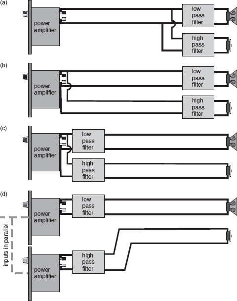
Figure 20.3:

Some wiring options for passive crossovers: (a) full-range, direct; (b) conventional bi-wiring, minimising the length of cable carrying full-range current; (c) bi-wiring with crossover filters remote from the loudspeakers; (d) amplifier inputs in parallel, poly-amplification, still using high-level, passive crossovers.

Cable conductor material is a source of continual debate. There does seem to be evidence that silver has subtle sonic benefits over copper, and that oxygen-free copper, especially of the long-crystal type, has benefits over standard copper. However, when loudspeaker cable lengths are kept to 2 m or below, and when the cables only carry band-filtered signals to individual drive units, the evidence for sonic differences between the conductor materials is scarce, especially if adequate cable cross-sections are used. For 8 Ω loudspeakers, 2.5 mm² cable is recommended for mid and high frequency drivers and 4 mm² cable for bass drivers. At 4 Ω, 6mm² cable would be advisable for low frequency drivers. It must be remembered that whilst doubling the length and cross-section may more or less maintain the same resistance value, doubling the cross-section can do nothing to lower the series inductance, which will increase proportionately to the length. Only very close coupling of the conductor pairs can reduce inductance. Coaxial cables can be useful here, and ordinary RG59 video cable can be very usefully applied to high frequency drivers as long as current demands are not too high.

Fuses in loudspeaker circuits are absolutely to be avoided. They do not have constant resistance; it will increase with temperature. The fuses can therefore act as limiters, increasing the series resistance as the drive current increases, and thus tending to oppose it. The fuses also have a time constant, which means that their own thermal capacity will ensure that the temperature changes always lag the current changes. Close to the blow current, non-linear distortion of the order of 4% has been measured. Carefully designed electronic protection circuits in dedicated amplifiers are a much better solution when loudspeaker protection is needed, but relays are also to be avoided in loudspeaker circuits because of a tendency for their contact resistance to change over time. Contaminated contacts can also act like diodes, introducing non-linear distortion into the loudspeaker drive signal.

Figure 20.3 shows four means of driving and cabling loudspeakers with passive crossovers. The first (a) is the most usual, but is also the worst from the point of view of cable performance. The second (b) is simple bi-wiring, which removes the low frequency current stresses from the cables carrying the high frequencies. The third (c) removes the crossover from the electromagnetically hostile environment of high power loudspeakers. The fourth (d) uses separate amplifiers to drive independently the high and low frequency filters and loudspeakers. Although in case (d) the two amplifiers receive and supply the same voltage drive, the current drawn from each of them is frequency dependent. This can reduce intermodulation distortion. It is known as poly-amplification, which is only one step away from bi-amplification and multi-amplification, where the crossovers are placed before the drive amplifiers.

20.6 Crossovers

Ideally it would be useful to have a single loudspeaker drive unit which possessed a response from 20 Hz to 20 kHz, flat to within a decibel, and capable of giving sufficient acoustic output for studio monitoring purposes.

Unfortunately, the laws of physics dictate that this cannot be so, because the requirements for low frequency radiation and high frequency radiation are very different. A high power, low frequency loudspeaker needs to be large if it is to be efficient, whilst a high frequency loudspeaker (of high or low power) needs to be small. We are therefore stuck with a situation whereby different frequency bands need to be handled by different drive units. The electrical dividing networks that are used to feed the appropriate frequency bands to each drive unit are commonly known as crossovers, although ‘frequency dividing networks’ is a more representatively accurate term. The term crossover relates to the way in which the electrical filter slopes superimpose at the dividing frequency, rather than describing the function that they perform (i.e. the filter slopes crossover, or overlap).

It was probably the mid-1970s before the full implications of the inherent problems in crossovers and their application to loudspeaker systems began to be realistically addressed. Until then, standard theoretical filters were largely used, without consideration for the practical repercussions of filter use. No filter can cut on or off abruptly. A filter rolls off, from a flat response to a slope determined by the time constants of the reactive elements of the network – the inductors and capacitors. The slopes tend towards regular numbers of decibels per octave, normally in multiples of 6 dB, which is a direct result of the behaviour of not only inductors and capacitors, but also of many mechanical systems, such as the loudspeaker drive units themselves.

The signal, therefore, does not suddenly switch from one drive unit to another as the crossover frequency is passed. There is an overlap where the slopes cross over, hence the name. If the slopes are set so that the high and low frequency sections are 3 dB down where they cross over, then they will tend to sum to full power at that frequency. There are also other types of crossover in common use which are 6 dB down at the crossover frequency. The voltages sum to unity and they can provide a flat axial response, but the power response would be 3 dB down at the crossover frequency. The first option would initially seem to be the logical solution, but group delays inherent in filter circuits cause time-shifts that prevent minimum-phase summation, rather like the room reflexion problems discussed in Chapter 11. In neither case can these time-shifted dips be equalised in the frequency domain, so monitor equalisers cannot help the situation.

The time shifts, which are related to the phase shifts, also tend to steer the combined wavefront from a loudspeaker system in directions other than at a normal to the front baffle plane. This is because a loudspeaker drive unit receiving a delayed signal, with respect to another drive unit in the same system, will behave as though it were farther away from the listener. It is like having two drive units on a baffle that is inclined with respect to the listener, so the wavefront radiates at a normal to the imaginary, inclined baffle. The axis of the flat frequency response will therefore not be directly in front of the loudspeaker, but inclined upwards or downwards. Many things about loudspeakers are not as obvious as most people tend to believe. Crossover responses can affect the directivity pattern of the combined loudspeaker system. This is why many hi-fi loudspeakers are seen to have staggered front baffles. The low frequency loudspeakers are the furthest forward, to compensate for the delayed signal that they receive. As the delay tends to increase with the filter slope and reducing frequency, a steep slope low frequency filter will cause considerable delay.

Many loudspeaker drive units have irregular responses outside of their normal frequency range of use. It is therefore advantageous to use reasonably steep filter slopes to avoid such ragged responses from superimposing themselves on the total signal. A 6 dB/octave crossover would mean that, with a 3 dB down point at the crossover frequency, the output would only be about 9 dB down one octave away from the crossover frequency. If a drive unit had a 5 dB response peak one octave away from the crossover point, then its response would only be 4 dB (9 dB – 5 dB) below the wanted signal level, and so the irregularities in the response could clearly be audible. Alternatively, a 72 dB/octave slope would solve the problem completely, but would introduce other problems, such as greater group delays and possible ringing problems from the high Q filters needed to achieve such a slope. Crossover slopes are therefore chosen as compromises, and there are indeed many options.

20.6.1 Passive Crossovers

The function of a crossover is to split the frequency bands and send only the appropriate frequencies to each drive unit – lows to the woofers, mids to the squawkers, highs to the tweeters, etc. Traditionally this was done with passive networks of inductors and capacitors placed between the amplifier output terminals and the loudspeaker drive units; usually inside the loudspeaker cabinet. Typical, historical networks are shown in Figure 20.4. The values of components were often chosen presuming that the loudspeakers were electrically like resistors, but in fact that is not the case, because they exhibit resistance, inductance and capacitance. Their input impedance (resistance plus reactance) therefore tends to vary with frequency, and two typical impedance curves are shown in Figure 20.5. The traditional crossovers were thus usually mismatched to the load impedance, and response flattening often took place with the ‘adjust on test’ addition of components.

Very few large studio monitor systems still use passive, high level crossovers. They are usually either relatively poor performers or extremely expensive. The overwhelming modern consensus is that passive high-level crossovers (as opposed to passive low-level crossovers – see later) are not appropriate for top quality studio monitoring. The Japanese TAD and Kinoshita monitors are still in current use at a high professional level, but the latter, with suitable amplifiers to drive the very complex impedance presented by the crossover components and drive units, cost around €50,000 each: €100,000 for a stereo monitor system. The electrolytic capacitors that the crossovers use have a life of about 10 years, and can be subject to changing values with age. For the people who like these monitors – and there are many – if they deliver the desired sound in small PA system quantities they will pay the price if they can afford it, but this type of approach is not really a modern day engineering solution.

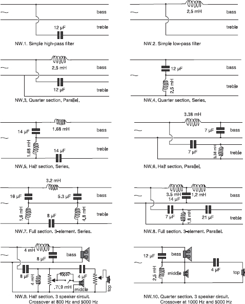
Figure 20.4:

Traditional crossover networks. Typical constant resistance crossover circuits with values for 15 Ω speakers and 1000 Hz crossover, except NW9 that is for 800 and 5000 Hz, and includes two volume controls and a switch for 2-way/3-way operation.

The problems are endless in the design of large monitor systems with passive crossovers. Amplifiers tend to need to be enormous, because, if they clip, the distortion products of the lower frequencies (which are usually the first to overload) are higher frequencies, and they pass straight into the high frequency drivers, often with very spiky waveforms. This can, and often does, produce premature failure of the high frequency drivers. In addition, the drive signals are passing one way through the filters whilst the back-e.m.f.’s (electro-motive-forces), created by the drive unit and filter resonances, are passing the other way through the filters. The complex impedances caused by this superposition can be almost beyond calculation; they are very signal dependent and they can put great strain on amplifiers. This is why the choice of amplifier can be so system-specific when driving passively crossed-over loudspeakers.

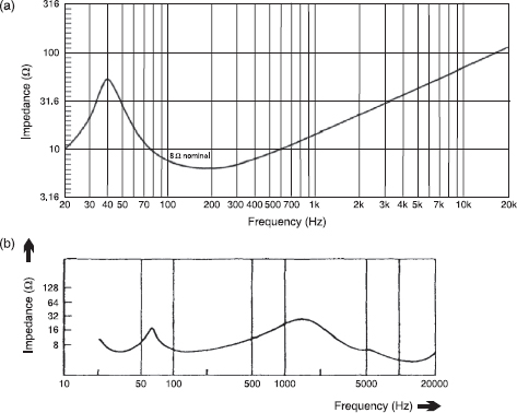
Figure 20.5:

Loudspeaker impedance curves: (a) Low frequency driver. Typical impedance curves for 8 Ω LF driver. Impedance shown on logarithmic scale (after Eargle); (b) A complete, full range loudspeaker system. KEF Model 104, impedance versus frequency.

As mentioned in the previous section, there are passive crossover designs that can fully compensate for the impedance variations with frequency. In one design, described by Colloms,² it is possible to maintain a 4 Ω input impedance, ± 0.5 Ω, between 20 Hz and 12 kHz. The three-way design uses a total of 11 inductors, 15 capacitors and four resistors, all to try to make the loudspeaker appear to the amplifier like a pure resistor. The possibility of being able to put so much between the amplifier and the loudspeaker drive units without negatively affecting the sonic performance would seem to stretch the imagination. To try to do this on a high power system, such as would be needed for studio monitoring, would be approaching the ridiculous. With capacitor values up to 600 microfarads, component drift with age would tend to lead to a very unpredictable response within a short period. This is perhaps why the Kinoshita solution was to let the input impedance vary, and look for a mega-amplifier to drive the 100 A currents that the loudspeakers occasionally demand.

The concept of the passive crossover can also be used at low levels, ahead of the power amplifiers, but they are rarely used. This is because once one has added the almost obligatory output driver stage (needed to cope with driving metres of cable, a range of amplifier input impedances, and balanced/unbalanced input/output configurations), it has already become an ‘active’ crossover, so one may as well incorporate the filter into the feedback circuitry. This then constitutes a typical, modern, active crossover, which offers many advantages.¹¹

20.6.2 Active Crossovers

Active crossovers can, by virtue of their feedback loops, remain very stable whilst also offering almost infinite possibilities of filter slopes. State-variable filters, even if they do drift, can cause the high and low pass filters to drift in unison, hence lumps or dips in the total response are avoided. Active filters can also easily incorporate delay compensation for driver mounting offsets, such as when a horn driver is set behind the woofers. Response tailoring is independent of the loudspeaker impedance complexities. The list of advantages in favour of active crossovers and multi-amplification is impressive:

1.  Loudspeaker drive units of different sensitivities may be used in one system, without the need for ‘lossy’ resistive networks or transformers. This can be advantageous because drive units of sonic compatibility may be electrically incompatible in passive systems.

2.  Distortions due to overload in any one band are captive within that band, and cannot affect any of the other drivers.

3.  Occasional low frequency overloads do not pass into the high frequency drivers, and instead of being objectionable, if slight, may be inaudible.

4.  Amplifier power and distortion characteristics can be optimally matched to the drive unit sensitivities and frequency ranges.

5.  Driver protection, if required, can be precisely tailored to the needs of each driver.

6.  Complex frequency-response curves can easily be realised in the electronics, to deliver flat (or as required) acoustic responses in front of the loudspeakers. Driver irregularities can, except if too sharp, be easily regularised.

7.  Complex load impedances are simplified, making amplifier performance (and the whole system performance) more predictable.

8.  System intermodulation distortion can be dramatically reduced.

9.  Cable problems can be significantly reduced.

10.  If mild low frequency clipping or limiting can be tolerated, much higher SPLs can be generated from the same drive units (vis-à-vis their use in passive systems) without subjective quality impairment.

11.  Modelling of thermal time constants can be incorporated into the drive amplifiers, helping to compensate for thermal compression by the drive units, although they cannot eliminate its effects.

12.  Low source impedances at the amplifier outputs can damp out-of-band resonances in drive units, which otherwise would be uncontrolled due to the passive crossover effectively buffering them away from the amplifier.

13.  Drive units are essentially voltage-controlled, which means that when coupled directly to a power amplifier (most of which act like voltage sources) they can be more optimally driven than when impedances are placed between the source and load, such as by passive crossovercomponents.

14.  Direct connection of the amplifier and loudspeaker is a useful distortion reducing system. It can eliminate the strange currents that can often flow in complex passive crossovers.

15.  Higher order filter slopes can easily be achieved without loss of system efficiency.

16.  Low frequency cabinet/driver alignments can be made possible which, by passive means, would be more or less out of the question.

17.  Drive unit production tolerances can easily be trimmed out.

18.  Driver ageing drift can easily be trimmed out.

19.  Subjectively, clarity and dynamic range are generally considered to be better on active systems compared to their passive equivalents (i.e. same boxes, same drive units).

20.  Out-of-band filters can easily be accommodated, if required.

21.  Amplifier design may be able to be simplified, sometimes to sonic benefit.

22.  In passive loudspeakers used at high levels, voice-coil heating will change the impedance of the drive units, which in turn will affect the crossover termination. Crossover frequencies, as well as levels, may dynamically shift. Actively crossed over loudspeakers are immune from this effect.

23.  Problems of inductor siting, to minimise interaction with drive unit voice coils at high current levels, are nullified.

24.  Active systems have the potential for the relatively simple application of motional feedback, which may come more into vogue as time passes.

Conversely, the list of benefits for the use of passive, high-level crossovers for large studio monitors would typically consist of:

1.  Reduced cost? Not necessarily, because several limited bandwidth amplifiers may be cheaper to produce than one large one capable of driving complex loads. (The loudspeaker may be cheaper but the system more expensive).

2.  Passive crossovers are less prone to being misadjusted by studio engineers. True, but in a professional studio one ought to be able to expect a degree of responsibility in the use of professional systems. However, passive systems have a tendency to mis-adjust themselves with age.

3.  Simplicity? Not really, because very high quality passive, high-level crossovers can be hellishly complicated to implement, not to mention the amplifiers which are needed to drive them.

4.  Self-containment of the loudspeaker system: but this is probably only interesting for hi-fi enthusiasts who wish to use them with their favourite amplifiers.

5.  Ruggedness? No; because the electrolytic capacitors (necessary for the large values) are notorious for ageing, and gradually changing their values.

Clearly, the advantages of active, low-level crossovers completely eclipse those of passive, high-level crossovers, yet it was only around the late 1980s that dedicated active crossovers began to be seriously used on large-scale monitor systems. Prior art used stock electronic crossovers and perhaps these caused some delay in the acceptance of totally active designs because they normally were made with fixed slopes on all the filter bands. It took some time before people generally began to accept the need to buy a specific, bespoke crossover with a monitor system, which could be relatively useless in any other application. There was still a mix-and-match mentality towards component parts, each of which was expected to function as a ‘standalone’ device. Once attitudes like this have become established it can be very difficult to introduce new concepts. In fact, it took a long time before self-powered, actively crossed over small monitors could establish their place in studio use. Domestic resistance to their acceptance has been even more pronounced. Established practices die hard, and they can be remarkably difficult to change, even in the face of clearly superior technology.

20.6.3 Crossover Characteristics

Crossovers are more than simple filters. Due to the group delays that exist in filter circuits, the outputs of the various filter sections are time-shifted by virtue of the phase shifts which are inextricably linked to the roll-offs. The result is that when the outputs are recombined, either electrically or acoustically, there are often non-minimum phase response irregularities in the frequency responses. Essentially, these have to be lived with, because they cannot be corrected by analogue means. Digital crossovers can be made to provide summing outputs, but the sonic benefits are not necessarily worth the effort and digital crossovers, unless they employ high sampling rates (96 kHz or more), will restrict the resolution in such a way that could make it difficult to accurately monitor some analogue or high sampling rate digital recordings. What is more, a three-way stereo crossover used with an analogue mixing console would require two A to D converters and six D to A converters. If these were to be of the highest quality (and in a high quality monitoring system they could be expected to be nothing less) the cost of the unit could be exorbitant. Using anything less than the finest converters would make a mockery of trying to monitor recordings made through the best converters. This subject is discussed further in Section 20.6.5.

Crossover output summation is a complicated affair. First-order (6dB/octave) crossovers can sum perfectly to reproduce a square wave applied to their inputs. This is because the 3 dB hump, which the in-phase outputs would be expected to produce at the crossover point, is exactly cancelled by the 3 dB dip which results from the ±45° phase shifts of the high and low pass section outputs. The step response of a 6 dB/octave crossover is shown in Figure 20.6. When the outputs of a two-way crossover using traditional second order filters (12 dB/octave) are connected in-phase, they produce a smooth phase response but a dip in the on-axis amplitude response. When connected out of phase (reverse polarity), the axial amplitude response is flat, but the phase response is kinked. As the phase and amplitude response must be flat in order to reproduce a transient accurately (see Section 11.5.3 and Glossary – Transient response) second-order crossovers cannot normally do so, no matter which way round they are connected. The effect on a step-function is shown in Figure 20.7. However, driver offsets at higher frequencies of crossover can sometimes reintroduce a better transient response, but this may require filters with asymmetrical turnover frequencies, such as used in the NS10M.

Third-order (18 dB/octave) and fourth-order (24 dB/octave) crossovers also cannot accurately reproduce transients, such as step-functions. However, due to the steeper slopes, the amplitude and phase response irregularities are confined to much narrower frequency bands, and hence are much less audible. The Butterworth (constant power) third-order crossovers produce slopes that are 3 dB down at the crossover point. The voltage outputs are in phase-quadrature (90° out) at all frequencies, by virtue of being shifted ± 135° in each direction. In fact, they are 270° out of phase when connected ‘in-phase’.

Another class of filter that is very popular with studio monitor designers is the fourth-order (24 dB/octave) Linkwitz-Riley crossover. These consist of two, second-order Butterworth sections in cascade. The in-phase connection gives a flat voltage summation, and can give a flat amplitude response on axis, but the nature of the filter’s total frequency response (phase and amplitude) is that it must give rise to the 3 dB dip in the total power response at the crossover frequency. This is not a practical problem in most control rooms, because in highly damped conditions the total power response is not of as much importance as the on-axis frequency response.

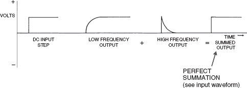
Figure 20.6:

First order (6 dB/octave) crossover step function summing.

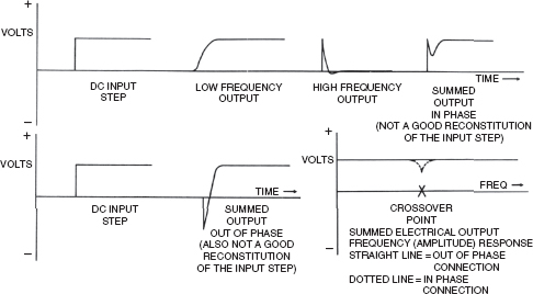
Figure 20.7:

Typical electrical step-function responses for 12 dB/octave crossover. Note that in-phase or out-of-phase, the summed output is not a true replication of the input waveform.

The range of available filter slopes and shapes is enormous, and detailed analysis of crossover design and performance is way outside the scope of this book. Readers needing a more in-depth study should refer to the Bibliography at the end of the chapter (especially Self [2011]). However, a few important characteristics can be considered here. Things will be discussed in terms of active, low-level crossovers and multi-amplification, because in the twenty-first century it appears to be very hard to justify the use of high-level passive crossovers in serious, new, studio monitor designs. Although there are some known and trusted monitors still in use with passive crossovers, it is unlikely that more will arrive. Despite the fact that the multi-amplified monitors took some time to fully establish themselves (monitoring has always been a rather conservative subject, and perhaps quite rightly so), once they took hold the benefits became so obviously apparent that older techniques are now rarely considered in new designs.

20.6.4 Slopes and Shapes

At least in analogue designs, the 6 dB/octave (first-order) Butterworth crossovers are the only ones that can truly reconstruct a transient waveform at their combined outputs. The main problem with their use is that their attenuation rate is so slow that out-of-band interference between the drivers can be a big acoustic problem. What is more, the slow rate of filter attenuation is not much use in protecting high frequency drivers from the damaging low frequency inputs. The only common use for 6 dB/octave filters is in ‘half-crossovers’, such as when a naturally tapering high frequency response of a mid-range driver is matched by an electrical filter which progressively brings a tweeter into circuit. There is another use for 6 dB/octave slopes in some complex, mixed slope, linear-phase/constant voltage crossovers, but the need for one driver to exhibit a flat response up to three octaves, or so, out of range makes such designs rather impracticable.

The 12 dB/octave (second-order) filter provides a good polar response, and has been used in many famous passive designs such as the Yamaha ‘NS10M Studio’. However, in many cases of their implementation, the problems involved with getting the transient responses adequately accurate have been a handicap. In passive designs, this type of filter was popular because it was cheap and simple, but in active designs, they hardly reduce the price or complexity at all.

The 18 dB/octave (third-order) crossovers, such as the Butterworth, are widely used, despite the asymmetric off-axis performance which results when using non-coincident drivers. Perversely, it has nearly always been the case with such designs, that they have not been used with coincident drivers.

The fourth-order Linkwitz-Riley (24 dB/octave) crossovers have come to be the generally preferred form, although their design is rarely straightforward in high-quality monitors. The electrical filters are usually designed to have a 24 dB/octave ‘target response’ when superimposed on the electroacoustic response of the drive units. The sequence of events for the design of crossovers for high-quality monitors therefore tends to be:

1.  Select the drivers for their sonic performance.

2.  Measure their responses around the crossover region.

3.  Design a filter that will give the desired ‘target function’ response in the room when feeding the appropriate driver.

In fact, the days of the use of standard electrical filters in crossovers are long gone. It is now almost universally recognised that the response shapes of the drivers themselves should be taken into account as part of the crossover filter design.

20.6.5 Digital Crossovers

Digital crossovers have seen increasing use as time has advanced. They are particularly attractive because of the relatively easy implementation of almost any amplitude response, phase response, delays, driver compensation and even room compensation. However, the big limitation to digital crossover use in studio monitoring systems is the cost of the converters. In any monitoring chain, the quality of response should be equal to or greater than the response in any other part of the system. If this is not so, then one cannot monitor the quality of the recording chain. It is difficult to measure to 140° C with a thermometer which only goes from 0 to 100° C. Likewise, if a studio purchases ultra-high-quality converters for any part of its recording or mixing chain, then the use of anything less in the monitor chain is an absurdity. One would not be able to hear how good the recording was, due to the limitations of the monitor converters. Surely, this ought to be self-evident, but it often appears to get overlooked.

As mentioned previously, but worth repeating here, a stereo, three-way digital crossover has two inputs and six outputs. For use with analogue mixing consoles, which at the time of writing still occupy the majority of ‘high-end’ studios, this would need two ultra-high-quality A to D converters, and six ultra-high-quality D to A converters. With a digital input, the six D to A converters would still be required to drive the power amplifiers. Even if digital crossovers are used with a digital mixing desk and amplifiers with digital inputs, then one must still ask questions about their (the amplifiers’) converter qualities, which are almost certainly likely to be less than the best.

Likewise, whatever sampling rates or bit-rates are in use, the electronics of the monitor circuitry should always be equal to or greater than anything anywhere else in the chain. For example, one could hardly expect to hear any benefit of 192 kHz sampling through a crossover based on 48 kHz sampling. These things all need to be carefully considered before choosing digital crossovers as an option for high-quality monitoring systems.

20.7 Loudspeaker Cabinets

The cabinets in which loudspeaker drive units are mounted are an important part of the loudspeaker as a whole. When an electrical drive signal enters the voice coil of a loudspeaker, the coil is attracted or repelled, depending on polarity, by the magnet system. However, the force which is produced by that motor system has no way of ‘knowing’ whether it is being resisted by the stiffness of the loudspeaker suspension system, the load imposed by the air in front of the diaphragm, or the spring which is formed by the air inside the loudspeaker cabinet. All it sees is the total impedance to its motion. That is why (as in many loudspeaker design books) the cabinet can be modelled by electrical symbols of capacitance, inductance and resistance.

A small loudspeaker cabinet will behave like a stiffer spring than a large one. Therefore, for two drive units of equal free-air resonant frequency, the stiffer spring of the smaller cabinet will force the resonant frequency upwards to a greater degree than would be the case for the identical driver in the larger box, hence restricting the low frequency response, which tends to roll-off below resonance. This can only be brought back down again by using a heavier cone, which will then need more power to move it. For an equal acoustic output over a given frequency range, smaller boxes need more power to drive them. Smaller boxes also usually have a greater difficulty in dissipating the heat from the voice coils, so the greater heat produced and the greater difficulty in getting rid of it can mean that smaller loudspeaker boxes are more prone to thermal compression effects when reproducing high levels of low frequencies. The thermal compression results from the rise in resistance of the copper or aluminium voice coil with increasing drive current. This increase in resistance prevents the coil from drawing as much current from the amplifiers, for any given output voltage, than a cold coil. The effect is exactly like that of a compressor. This concept is discussed further in Section 20.8.2. Whilst it is true that circuitry could be used to model the compression and partially compensate for it, this would require more voltage from the amplifiers, so even larger amplifiers may be necessary, probably needing more power still, so efficiency reduces further.

There is, effectively, an ‘eternal triangle’ of size, efficiency and frequency range. Whenever size is reduced, then for a flat response, either the efficiency of the loudspeaker system or its low frequency extension must also reduce. In most cases, both reduce with size. Therefore, it is not that one cannot generate very low frequencies from small boxes; it is just that one cannot do it efficiently. Hence the sensitivity difference between the large UREI 815 and the small ATC SCM10, described in Section 20.4. For high levels of extended low frequencies, from reasonable amplifier power, loudspeakers must be large. This is somewhat like the fact that a double bass needs to be much larger than a violin. The need for large low frequency sources will be discussed further in the following section on loudspeaker drive units.

Large cabinets have large areas of cabinet walls, and with high internal pressures being generated by the drive units it can be difficult to prevent the walls from vibrating. The problem with panel vibrations is that they act as secondary radiation sources, and the secondary radiation can seriously colour the sound by adding to or subtracting from the direct radiation from the driver(s). Panel vibration therefore needs to be minimised, which calls for high rigidity and damping. Usually, that double requirement means that there will need to be considerable mass – the cabinets will be heavy. For commercial reasons, monitor loudspeakers intended for large-scale sales often tend to be lighter than acoustically optimum. Transport costs and handling difficulties would make very heavy cabinets more expensive and less manageable, and hence less likely to sell in large quantities. Conversely, some specialised studio monitors which are solely intended for flush mounting, and which were not intended to be mass-market products, never need to be compromised by marketing considerations and so can be enormously heavy, to good advantage.

20.7.1 Cabinet Mounting

The difference in cabinet weights and rigidity leads to two common approaches to mounting the loudspeakers in a monitor wall. The lighter cabinets are usually more subject to panel vibration problems, which can pass into a control room structure if rigidly mounted. This can lead to vibration passing through the structural materials at speeds much faster than through the air. These vibrations can re-radiate from parts of the structure and form secondary sources, sometimes arriving at the ear before the direct sound.³ The usual answer to this problem is either to resiliently mount the loudspeakers, on rubber for example, or to try to substantially damp the cabinet walls by encasing them in concrete. The much heavier, specialist loudspeakers, because of their highly damped massive nature, need less special attention, as their external cabinet vibration levels are usually insignificant.

Many hi-fi enthusiasts mount their loudspeakers on spikes, which bite into a wooden floor. In some cases, this is to prevent recoil effects if the loudspeakers are mounted on carpet. When the bass drivers punch in and out, there can be cabinet reactions which, if mounted on carpet, could cause the whole cabinet to shift forwards and backwards sufficiently to cause phase modulation of the tweeter response, hence blurring the high frequencies. Spikes penetrate the carpet to get a solid fixing on the floor below. Spikes are also sometimes used directly on wooden floors to avoid rattles, which may occur due to the imperfect contact between the flat underside of the loudspeaker (or its stand) and the floor boarding. Spikes are therefore often a solution for light to medium weight cabinets. With very heavy and well-damped cabinets, the problems do not usually arise.

Whilst on the subject of loudspeaker mounting, a little should be said about the height at which they should be positioned in a wall. The general tendency amongst most careful designers is to site the mid-range units approximately 145–148 cm above the floor. This is a mid position between the ear height of a small person sitting down and a tall person standing up. It minimises the variability in frequency balance as people move around the room, or move out of their chair to a standing position. It also ensures that the sound enters the ears from a natural direction during most operations. The practice of mounting monitor loudspeakers high is to be discouraged, because in a normal, slightly nose down working position for the people at the mixing console, the sound from high-mounted monitors tends to arrive at the ears from a direction perpendicular to the top of a person’s head, as shown in Figure 18.6. Both high frequency perception and stereo imaging can be badly affected, and the reflexions created by the working surface of the mixing console can muddy the sound.

It should be recognised that differences in control room sizes and design philosophies can modify the requirement to some degree, but there is now great consensus amongst designers that the 145–148 cm (4 foot 9 inches to 4 foot 10 inches) mounting height, with the monitor cabinet baffles vertical (i.e. no inclination) is the best compromise. The concept is shown diagrammatically in Figure 20.8.

The horizontal placement of the cabinets can be influenced by window positions and sizes, and the need to maintain the chosen subtended angle at the listening position. However, one thing which is almost standard practice is to focus the monitors at a point about 60 to 80 cm behind the principal listening position. This barely compromises the stereo at the prime listening position, but it significantly enlarges the area in which people can sit side-by-side at the mixing console and still more or less hear the same stereo panorama. Figure 16.7 shows the general idea.

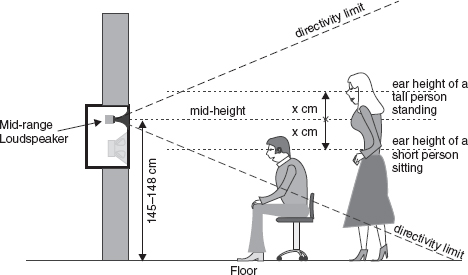
Figure 20.8:

By mounting the loudspeakers vertically, and not inclined, the height of the mid-range loudspeakers can be set between the ear heights of a small person sitting and a tall person standing. Only by mounting the loudspeakers vertically can this condition be maintained throughout the room. Such mounting is also less likely to cause reflexions from the upper surface of the mixing consoles.

20.7.2 Cabinet Concepts

Loudspeaker cabinets are huge subjects in themselves, and they are very much a part of the loudspeaker electroacoustic system. They are not merely convenient boxes in which to mount the drive units. A good understanding of the concepts is very useful in aiding the better application of the most appropriate choices. The main point to bear in mind is the way that the loudspeaker mounting conditions have a large effect on the overall system performance, and that the mounting conditions are, essentially, a part of the loudspeakers themselves. The Bibliography lists sources where this subject is taken much further.

As few, if any, recording studios now work on large monitors alone, the mounting conditions for the small loudspeakers need some consideration, or their performance will not be optimal. Figure 20.9 shows the adverse effects commonly found when mounting small loudspeakers on console meter bridges. Mounting the loudspeakers on stands, behind the console, can go a long way to reducing such reflexion problems; however, the low frequency response of the two mounting systems can be very different. Depending upon the nature of the structure of the console, the physical contact between the flat surface and the loudspeaker can either reinforce the low frequencies if the console is rigid, or reduce the low frequencies if the console is significantly resonant. As so many different situations exist, it is hard to specify specific rights and wrongs. Nevertheless, a very good way of determining the best mounting position for small loudspeakers is to have two people hold one loudspeaker each, against their chests, and walk from a distance of about 1m behind the console towards the listening position, as shown in Figure 20.10. If the loudspeakers are finally placed simultaneously on the meter bridge, any sudden change in the timbre of the sound could be attributable to structural or cavity resonances in the console. In many cases, as the people bring the loudspeakers closer to the console, great changes can be noticed in the clarity of the sound and the stereo imaging. Colouration often increases the closer the cabinets are to the meter bridge, due to reflexion and diffraction effects.

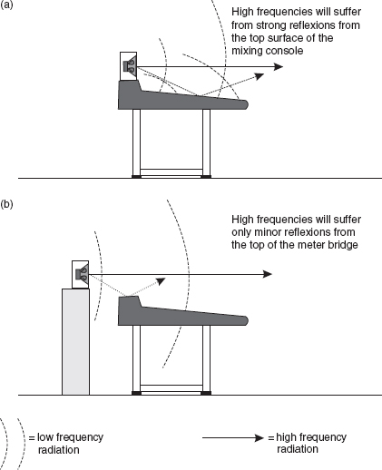
Figure 20.9:

Small loudspeaker mounting: (a) Small loudspeakers mounted on top of the meter bridge will suffer low frequency reinforcement because the low frequency waves are not free to expand. They are constrained by the close presence of the mixing console (this may or may not be a bad thing); (b) Low frequencies will be more free to expand, so they will tend to be weaker than for loudspeakers mounted on the meter bridge. Situation (b) is generally preferable unless the loudspeakers are somewhat lacking in bass.

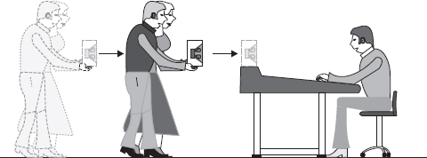
Figure 20.10:

Two people can hold one loudspeaker each, walk towards the mixing console from a position a metre, or so, behind the console, and finally put the loudspeakers on the meter bridge. Care should be taken to ensure that the two people (holding the left and right loudspeakers) move in unison. Any changes in frequency balance, colouration, or stereo imaging should be clearly heard by the listener sat in the engineer’s position.

By using this method, an optimum position for the small loudspeakers can usually be easily chosen. However, distances of more than 30 cm or so from the rear of the console may necessitate the covering of the back of the console with an absorbent material, to prevent potentially disturbing reflexions from the console returning to a front window, for example, and reflecting back to the listening position. As the mounting of an absorbent screen behind the console is also generally good practice from the point of view of the main monitoring, it should not be seen as a disadvantage to the more distant mounting of the small loudspeakers. It must be borne in mind, though, that moving the small loudspeakers from a distance of 1 m to a distance of 2 m from the listening position could require 3–6dB more drive – up to four times the amplifier power – due to the doubling of the distance from the listening position.

20.7.3 Mounting Practices and Bass Roll-Offs

In small control rooms, the proximity of the loudspeakers to the front wall can cause a bass boost, as discussed in Chapter 11. In the case of reflex enclosures, the rise can sometimes be compensated for by the blocking of the tuning port(s). The consequent reduction of the low frequency output from the port can often offset the rise due to the proximity of a wall. This is a perfectly legitimate exercise, because it is the response perceived at the listening position which is all-important. However, it will tend to change the slope of the ultimate low frequency roll-off, and it may affect the ventilation and heat loss from the voice coils.

A loudspeaker on an open baffle board will suffer a low frequency roll-off from a frequency set by the cancellation around the sides of the baffle, and hence by the baffle size. For practical sized baffles, this will begin from quite a high frequency, but the roll-off will only gradually fall to 18 dB per octave. In the case of a sealed box, the frequency where the roll-off begins can be reduced compared to the same drive unit on an open baffle, and the slope will tend towards 12 dB per octave. With reflex tuning of a similar sized box, the roll-off can be delayed until still lower frequencies, but once the roll-off begins, it will attain a slope of 24 dB per octave.

Different types of loudspeaker cabinets therefore have different characteristic low frequency roll-off slopes, and hence, not surprisingly, different characteristic sounds. This is even less surprising when one considers that the slope of the roll-off also affects the time response, with the steeper slopes giving rise to more signal delay in the region of the cut-off frequency. (See Figure 19.11.) The fastest transient responses are exhibited by the loudspeakers with the shallower roll-offs. Work carried out in 2001 at the Institute of Sound and Vibration Research, in the UK, has shown that above 30 Hz, the subjective colouration due to steep roll-offs can be considerable. However, the roll-off rate itself is not the whole story. Bank and Wright⁴ have noted that despite the bass reflex and transmission line cabinets both exhibiting a 24 dB per octave roll-off, the subjective perception of their low frequency responses can be quite different. It is thus necessary to appreciate how some seemingly simple changes in loudspeakers can have some disproportionately complex results.

Intuitively, blocking the port on a loudspeaker would suggest that the drive units would be better protected from low frequency overloads by virtue of the pressure changes inside the cabinet during high excursions. In fact, at resonance, a loudspeaker in a vented (reflex) enclosure moves much less than a similar driver does in a sealed box of equal size. Down to the resonant frequency, a vented enclosure actually protects a driver better than a sealed box, although below resonance all control is lost. This is why small, ported loudspeakers intended for high-level use often have steep filters to protect them from excessive drive below their useful operating frequency band. Despite their widespread use in modern actively driven (built-in amplifier type) loudspeakers, such filters do colour the sound of the low frequencies, and can cause severe deterioration of the transient response. Figure 19.4 shows the effect of cabinet tuning and low frequency alignment on the acoustic source positions.

20.8 Loudspeaker Drive Units

The drive units (or motor systems) of loudspeakers are at the core of any studio monitoring system. The needs of low frequency and high frequency sound radiation are very different, and therefore for high-quality loudspeaker systems more than one drive unit is required to cover the entire audible frequency range. Low frequency drivers need to be large, because they need to move a large volume of air. Most dynamic loudspeakers are volume/velocity sources, where the acoustic output is the product of the two. So, at low frequencies, where cone velocities are small, the volume of air which needs to be moved is proportionately larger than at high frequencies, where the vibrational velocities are much higher. The acoustic requirements of a conventional high frequency loudspeaker require it to be small, in order that the high frequencies will be well distributed. If the radiating surface were to be large, then the parts of the sound arriving from different parts of the surface could have considerable phase shift at high frequencies, where wavelengths are short. At 20 kHz, the wavelength is around 1.7 cm, so if the difference in path length from the ear to two different parts of the radiating surface were only 8 millimetres, the radiation from the two places would arrive at the ear 180° out of phase, and so would cancel.

20.8.1 Low Frequency Driver Considerations

In general, larger low frequency drivers tend to be preferable to smaller ones for any given radiated output level. If the volume-velocity product is to be the same, an 8 inch (20 cm) diameter loudspeaker would need to travel much further than an 18 inch (45 cm) loudspeaker for each cycle of the music. An 18 inch loudspeaker cone has a surface area of 254 in², whereas an 8 inch loudspeaker cone has a surface area of only 50 in². In order to displace the same amount of air, the smaller cone would have to move five times the distance of the larger cone, and would need to travel at five times the speed in order to displace the same amount of air in the same amount of time. The difference has several implications.

When higher frequencies are simultaneously being radiated from a cone that is undergoing low frequency excursions, frequency modulation can take place due to the Doppler effects (see Glossary). Obviously, a large cone moving slowly over short distances will produce far less Doppler shift (frequency modulation) than a small cone moving rapidly over greater distances. Furthermore, a small cone punching its way violently through the air will create far more turbulence at its edges than a large cone moving slowly. The implication of this is that spurious noise generation is far less likely in the case of the larger cone. Another point to consider is that loudspeaker suspension systems and magnet systems can be notoriously non-linear, and the degree of non-linearity tends to be proportional to the distance travelled. It is thus generally easier to keep non-linear distortions lower in low displacement large cones than in high displacement small cones for similar acoustic outputs.

There are limits to woofer size, however, because the cones can be very difficult to keep rigid once their diameter increases beyond 45 cm (18 inches). The tendency is therefore to use more woofers of the same size when output needs to be augmented, rather than a single driver of greater size. Some woofers designed to operate to relatively high frequencies – say 500 to 1000 Hz – are specifically designed to decouple concentrically the outer parts of the cone from the centre section as the frequency rises. Such decoupling prevents the phase cancellation effects described earlier, when the source size becomes large with respect to a wavelength of the frequency being generated. Ideally, by 500 Hz, the radiating proportion of a large cone would need to be only the central portion of about 25 cm in diameter. If such internal cone decoupling cannot be achieved, then the only solution is to cross-over into a different drive unit of smaller diameter. If this is not done, the large cone will begin to emit the higher frequencies in a narrow beam, which would give rise to undesirable off-axis frequency responses and a narrower usable listening area.

20.8.2 Efficiency and Sensitivity

These two loudspeaker parameters often get confused. Efficiency is the degree to which a loudspeaker can convert its total electrical input energy into acoustic output energy. The sensitivity describes the acoustic output of a loudspeaker, on-axis, at a given distance (usually 1m) for a given electrical input (usually 1 W, or 2.83 V [the voltage equivalent of 1 W into 8 Ω]) in its operational frequency range.

Sensitivity and efficiency are important in that their absence creates problems. Inefficient, insensitive drivers need a lot of electrical power input in order to achieve an adequate sound output. A woofer with a 500 W power rating and 0.5% efficiency will, at full power, dissipate 99.5% of its input power – or 497.5 W – as heat within its voice coil and magnet system. Hence, the blackened magnets and chassis heat sinks to be found in many high power loudspeakers: the black colour helps to radiate the unwanted heat into the air. A loudspeaker with a sensitivity of 85 dB for 1 W at 1 m, dissipating 400 W, would produce the same acoustic output as a loudspeaker with a sensitivity of 95 dB for 1 W at 1m dissipating 40 W. The 10 dB difference represents a ten times power difference and losing 40 W to the atmosphere is much easier than losing 400 W. Consequently, for the same given output power, the 95 dB loudspeaker would run much cooler than the 85 dB loudspeaker. The principal significance of this is that a typical copper voice coil resistance increases by about 0.4% per °C. As the resistance rises, the ability to draw current from a typical amplifier reduces, so more drive voltage is needed to maintain the output from a hot coil when compared to a cold coil. As most amplifiers do not know the temperature of the coil that they are driving, the usual result is that as the voice coil temperature rises, the acoustic output falls. This is known as thermal compression. A temperature rise of 250°C will double the coil resistance, and many inefficient loudspeakers do work at temperatures of 250–300°C. Three or four dBs of compression under such circumstances would be typical. In conventional voltage driven loudspeakers, there is no total solution to thermal compression, so if a loudspeaker will be subjected to moderately high-level sustained outputs, the compression can only be avoided by using drivers of greater sensitivity, or fan cooling the chassis.

Many of the woofers used in commercial monitor systems are of relatively low sensitivity, because of a commonly held view that amplifier power is cheap, whereas powerful magnet systems are expensive. Almost nothing is now free of cost restraints, and the price at the point of sale is the god. Nevertheless, over the years, the cost of the extra electricity consumption needed to drive the low sensitivity loudspeakers will also add up to a considerable amount, but hidden costs such as these are usually ignored, despite being very real. In fact, in the long-term, and after the receipt of many electricity bills, it may be realised that amplifier power is not cheap. What is more, in many countries, obtaining high current electricity supplies is difficult and expensive, and in hot climates, extra power for the amplifiers means extra power for the air-conditioning to take out the heat that the amplifiers are pumping into the control room. In many circumstances, these problems are not trivial.

20.8.3 Magnet Systems and Cone Materials

When Zambia became an independent country in the 1970s, a civil war broke out. Zambia produced around 80% of the world’s cobalt, an important constituent of most high-quality loudspeaker magnets at that time. Many of the mines became flooded during the war, and consequently the price of cobalt on the world market rose enormously. So much so, in fact by about 2000%, that the majority of the world’s loudspeaker manufacturers began to look for magnet materials other than the Alnico (aluminium/nickel/cobalt [with copper and iron]) which was becoming so expensive. Other magnet materials, such as Ticonal and Alcomax, also contained cobalt (the former also with titanium), and so suffered large price rises.

The industry generally turned to a range of barium or strontium ferrites, which were ceramic, non-conducting materials. They were also cheap. However, the physical shapes and sizes needed for the new ferrite magnets often meant totally redesigning the motor systems. A serious problem with ferrite magnets, which was not at first appreciated, was due to their non-conducting nature. This was the inability of the magnetic material to provide an electrical short circuit to eddy currents derived from the interaction of the magnetic fields of the coil and the magnet itself. The flux consequently moves in a series of jumps, rather than smoothly. The result can give rise to a form of programme-modulated noise, somewhat similar to modulation noise on magnetic tape recordings. If the magnetic material is conductive, then any magnetic field changes need to generate large eddy currents in the electrical short circuit provided by the metallic magnet, and are thus smoothed out.

For many years, audiophiles have extolled the virtues of the older magnets, and only recently has the explanation become more commonly understood. Ferrite magnets can therefore exhibit a ‘bit-rate’ that limits their resolution. Hence it is not only the weight saving which has spurred on many manufacturers to use the newer rare-earth magnet materials, such as neodymium/iron/boron and samarium/cobalt (yes, back to cobalt again, but in smaller quantities). In fact some of the newer magnet materials demand high sensitivities if they are for high output use, because they tend to demagnetise at high temperatures. The use of ferrites led to so much bad design partly due to their tolerance of high temperatures without demagnetising. Notwithstanding all of this, there are some good loudspeakers which employ ferrite magnets, although they also tend to employ special mechanisms to overcome the problems.

Cone materials can also significantly affect resolution, and pulped paper cones can still give a good account of themselves from this point of view. Many modern materials have been chosen for their physical properties in relation to their ability to perform as ideal pistons, but some low-level hysteresis losses within the materials can produce a rather similar type of programme-modulated noise that can result from the use of poorly designed ferrite magnets. Despite the measured performance of some ferrite-magnet/composite-cone low frequency loudspeakers being highly impressive, the subjective performance of some of the metal-magnet/pulp-cone loudspeakers is often considered to be more ‘open’ and ‘transparent’, probably due to the lower levels of programme induced artefacts. However, the degree of subjective differences can be heavily dependent on the frequency range being handled by the woofer. When the upper limit is restricted to 200 Hz or so, the subjective differences are greatly reduced, both for the magnetic material and cone material choices.

20.8.4 High Frequency Loudspeakers

The physics of high frequency sound reproduction demand that the surface area of the generating diaphragm should be small. There is now an enormous range of high frequency loudspeaker types, but in recording studio use, the general tendency is for the use of cones, domes, compression-driver/horn combinations, ribbon loudspeakers and Heil air-motion transformers. Somewhat rarely, Manger drivers are also to be found (see Section 20.8.5.4). One of the greatest controversies is usually in the choice of hard or soft materials for the domes. Hard domes may be made from titanium, aluminium, beryllium, copper and plastics of various natures. Phenolic-doped fabrics have also been employed. Soft domes are usually made from fabrics, suitably doped with rubbery materials which impart to them the desired stiffness and damping.

The precise choice of high frequency drive unit in any given system is highly subjective, with some manufacturers adopting specific types with almost religious fervour, whilst eschewing the favourite choices of other manufacturers. Marketing also has a great deal to do with this, where one manufacturer wants to impose on its products a recognisable brand image, which it can then sell for all it is worth. Unfortunately, this often does little for the benefit of the professional user.

Domes, cones and ribbons are usually relatively low sensitivity devices, and because they need to be small for sound radiation purposes, their ability to lose heat is often restricted. Sensitivities in the 90 dB for 1 W at 1m are typical, and ferro-fluid is often used, these days, to aid voice coil cooling. However, the stability of long-term performance of ferro-fluids is still not accurately determined, and may be environmentally dependent. The result is that at high levels, the effectiveness of cone, dome and ribbon drivers is limited, and at levels of 105 dB or so, many of them are reaching the limits of their linear operation. For higher levels of use, the only solution is either to restrict the high frequency driver to very high frequencies and use more crossover points, or to use horn loaded tweeters, yielding sensitivities as high as 108 dB for 1 W at 1 m. The disadvantage to the latter case is normally only cost, because little controversy exists about the use of horns above 7 or 8 kHz.

It also should also be noted that, contrary to much widely accepted mythology, dome tweeters do not exhibit better sound dispersion at high frequencies. The dome shape gives many people the idea of a section of a spherical radiator, but a dome can move in one plane only, and often tends to act more like a ring diaphragm, exhibiting a rather strange directivity. This subject will be dealt with in more detail in Section 20.8.5.2. Once again, as is so common in electroacoustics, things are often very different to what ‘common sense’ would tend to suggest.

One of the greatest influences on the sound from high frequency drivers is the design concept of the entire loudspeaker system. As discussed in Chapter 19, there is no universally accepted standard high frequency response for monitoring systems, and the subjective sound of two different tweeters may be dictated as much by the way that they are being used and the frequency response contour of the entire system as by the inherent properties of the high frequency drive units themselves. It has even been reported how adverse criticisms have been made of high frequency drivers operating above 6 kHz, when the source of the subjective harshness was found to be due to distortions in the low-mid-frequency drivers, operating only below 1.2 kHz.⁵ One has to be very careful before pronouncing judgement on almost any part of a monitor system, because the roots of many ‘obvious’ problems are very often not obvious at all.

20.8.5 Mid-Range Loudspeakers

This is a controversial subject; of that, there is no doubt. In many ways, this is not surprising, because it covers the range of maximum hearing sensitivity and the most significant range of musical instrument timbre. In general, for use in medium to large size studio monitors, the choice lies between cones, soft domes and horns, although hard domes do occasionally find use, especially in medium-sized systems. The mid-range of audio frequencies can probably be considered to span the range from 300 Hz to 5 kHz, which covers about four octaves. The whole range is rarely covered by a single drive unit, because the physics of sound reproduction usually dictates that a crossover occurs in the region.

A 500 Hz wavelength is around 67 cm, which is larger than the diameter of most low frequency loudspeakers. This means that low frequency loudspeakers are generally small compared to all of the wavelengths that they are radiating. By 4 kHz, however, the wavelength is only about 8 cm, which is small by comparison to the diameter of the typical cone or dome loudspeakers that would be needed for high level radiation (110 dB SPL+) of signals in the 500 Hz region. Because of the off-axis phase cancellation for 8cm wavelengths being generated by 20 cm diameter cones, the directivity would tend to become too narrow for studio use. There are therefore problems in covering the whole mid frequency range with a suitable drive unit for high level, high-quality monitoring, although the horn-loaded Kinoshitas go from about 500 Hz to 20 kHz with a single, though phenomenally expensive, compression-driver/horn combination. (See Figure 20.1(a).)

20.8.5.1 Cone drivers

Cones and domes are both used in domestic high fidelity loudspeakers covering the entire mid-range, but such small units can rarely be capable of dissipating the waste heat in high-level systems. Cones have always been a popular choice for mid-range drivers, and they have the rather fortunate tendency to break up in such a way that the higher frequencies are often decoupled from the outer edges of the cone, and thus tend to radiate from the smaller diameter central section. They can thus maintain their wide directivity as the frequency rises. Figure 20.11 shows two small mid-range cone drivers covering the mid frequency range in a high power monitor system, but here they have been fitted with ‘noses’ and mounted in a shallow waveguide. The combination of the nose and waveguide lead to what is really a form of horn loading, which helps to augment the sensitivity of the system and also helps to control the directivity, both of which are desirable assets. Such a system of mounting provides the option of rotating part of the baffle through 90°, thus allowing the use of the cabinet either horizontally or vertically. Generally, the restriction of the use of cone drivers in high-level studio monitor mid-range use is because of the limit to the amount of heat that can be dissipated by the relatively small coils that tend to be used. Theoretically, however, there would seem to be no reason why small cones cannot be driven by larger than normal diameter voice coils, as has been pointed out by Watkinson.⁶

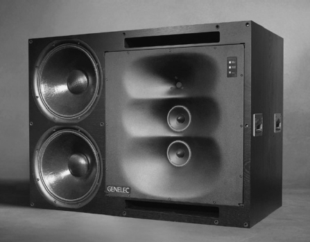
Figure 20.11:

The Genelec 1035B monitor loudspeaker. Note the ‘noses’ in the centre of the small mid frequency cone loudspeakers, and the sculpted waveguide into which they are set.

Colloms⁷ has noted that some cone materials can lead to unpleasant distortions at high levels due to gross compression and rarefaction stresses at the neck of the cone. This effect is most noticeable with certain types of plastic cone materials. He has also noted that the choice of cone material requires serious subjective testing, as well as objective analysis, because standard mid-range cones generally operate in a controlled break-up mode. This inevitably adds a degree of colouration to the sound which is characteristic of the particular material employed. ‘A sonic signature of the chosen materials technology’, as he puts it.

20.8.5.2 Dome drivers

Hard dome drivers, such as the beryllium dome used by Yamaha in the NS1000 loudspeaker, can produce outstandingly low distortion levels, but once they do break up, at high levels, they can do so rather aggressively. In high level monitoring, the soft dome has been fashionable now since around 1980.

The serious soft dome mid-range concept dates back to the work of Bill Woodman at ATC in England in the late 1970s. His 75 mm diameter unit was revolutionary in its time, and it could cover the range of about 400 Hz to 5 kHz with high output level, low power compression, low distortion and reasonably high efficiency. The dome was made of a doped soft fabric with a coil attached to its perimeter. A dual suspension system, somewhat unusual in previous domes, ensured a good pistonic performance. This dome was also used in early Quested monitoring systems. Stanley Kelly later designed a 100 mm unit for use in the Discrete Research ‘Boxer’ systems. ATC and PMC also had considerable success with their monitor systems using soft dome mid-range units in the 1990s and beyond.

The soft domes spawned an entirely erroneous, widespread belief that they had significantly better sound dispersion than cones. As previously mentioned in Section 20.8.4, their hemispherical shape suggested to many people that the sound radiated as in Figure 20.12(a), but in fact, as they move in one plane only, their action is pistonic, as shown in Figure 20.12(b). However, once they enter break-up, the centre of the dome uncouples from the high frequencies, contrary to the behaviour of a cone loudspeaker, because the dome is driven from its edges. The rather undesirable result of this is that the dome becomes a ring radiator, which lends to response beaming at high frequencies, because an annular radiator behaves like separate displaced radiators with a space between them, the centre of the ring being the null point.

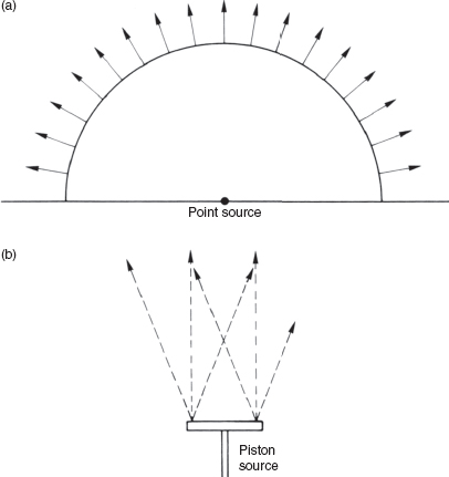
Figure 20.12:

(a) Spherical expanding wave with all particles moving away from each other; (b) single plane, pistonic movement, characterises radiation from dome loudspeakers. Typical directivity is that of equally sized cone loudspeakers.
The radiation shown in (a) would be typical of that from a pulsating sphere, and to some degree from many horns. A dome, however, although appearing like a hemisphere, does not pulsate. It moves backwards and forwards, in one plane only, and hence acts more like the piston shown in (b). At higher frequencies, if the centre of the cone decouples from the outer diameter, the driven portion acts like a ring diaphragm and radiates only from its perimeter. Radiating pistons produce particle motions that can interfere with each other, producing interference patterns and subsequent lobing of the polar pattern plots.

The more expensive dome radiators can produce excellent results, but they need careful attention to many aspects of their design. The lightweight domes are usually quite transparent to sound, so unless the cavity behind the dome is well damped, the rear radiation can colour the sound. Adequate damping requires expensive magnet systems, and these are sometimes hollowed and/or tapered to reduce resonance effects. Cheap ‘look-alike’ copies should be avoided, because the production of high-quality mid-range dome loudspeakers is difficult and expensive. The success of the better domes has largely been due to the ability to use large voice coils and large magnet systems, which have yielded high sensitivity and good heat dissipation. Good design also requires critical damping of the dome, itself, with viscous plasticisers.

The radiation shown in (a) would be typical of that from a pulsating sphere, and to some degree from many horns. A dome, however, although appearing like a hemisphere, does not pulsate. It moves backwards and forwards, in one plane only, and hence acts more like the piston shown in (b). At higher frequencies, if the centre of the cone decouples from the outer diameter, the driven portion acts like a ring diaphragm and radiates only from its perimeter. Radiating pistons produce particle motions that can interfere with each other, producing interference patterns and subsequent lobing of the polar pattern plots.

The enormous Community M4 loudspeaker has been used as a dome in some custom designed monitor systems. It was really designed as a compression driver, but it has seen use without its phase plug and mounted on a vestigial horn. Meyer, in some of their mid-field cabinets, has also used dome drivers at the throat of horns for the upper mid-range/high frequency part of the spectrum. In fact, most of the high power dome units employ a very short horn around the dome, which, although not appearing like stereotype horns, are horns nonetheless.

20.8.5.3 Mid-range horn loudspeakers

Perhaps nothing in the discussion of studio monitoring loudspeakers excites so much argument and passion as the question of the use of horn loudspeakers. For many people involved in recording, they are ‘The Devil Incarnate’, yet for many other people they are their optimal choice. It has to be said that many badly designed horn systems have been marketed over the 70 years, or so, of their use. Compared with the domestic hi-fi and public address markets, high-level studio monitoring is a very small market for loudspeaker manufacturers. It is therefore of little surprise that it has been forced to borrow much of its technology from the research done for the exploitation of the larger markets. Many large loudspeaker systems for studio use have directly adopted components from public address systems, and mid-range horns and compression drivers have been no exception. Despite the prime necessities of the two uses often being very different, many large-scale monitor systems have historically used unmodified components designed for sound reinforcement in concert halls and stadia. If the use of such systems has led to the widespread opinion that horns are undesirable as mid-range units in studio monitoring systems, it is not surprising. Then again, nor is it necessarily true.

Carefully and specifically designed horns for studio monitoring systems can be excellent performers, at low levels as well as high levels. Shown in Figure 21.3 is a monitoring system with a purpose designed mid-range horn/driver combination that does not possess a horn-like sound. However, there are limits to horn design which must not be transgressed if a natural sound is to be the result, and these can place restrictions on the shape and frequency range of the highest quality horns. In general, the rules are as follows:^8–10

1.  The distance from the diaphragm to the mouth of the horn should not exceed 35 cm, or thereabouts. (Magnet system design can determine the distance from the diaphragm to the throat, typically 0–10 cm.)

2.  Horn mouths should flare as smoothly as possible into the front baffle, avoiding sudden discontinuities.

3.  The flare rate determines the cut-off frequency, so to flare from a 25 bmm (1 inch) throat to a smooth encounter with the front baffle in no more than 35 cm of length requires a highflare rate, such that cut-off frequencies below 1 kHz are difficult, if not impossible, to achieve if the highest sonic resolution is the goal.

4.  To minimise internal disturbances that can give rise to both on and off-axis response anomalies, all corners, angles and obstructions in the horn should be avoided.

5.  Discontinuities in the throat region should be avoided, which makes the design of dual concentric arrangements somewhat difficult if they need to have gaps for the low frequency voice coils.

6.  The compression driver throat should not diverge from the flare angle at the throat of the horn. The transition from driver flare to horn flare should be smooth. Therefore, replacing one driver with another of different internal throat flare will not give fair comparisons, because they cannot both be optimally matched.

The last of the points mentioned above means that not all 1 inch-exit drivers will match all 1 inch (25 mm) horn throats. The smoothness of flare rate across the junction is of great importance if honky sounds are to be avoided. In the past, some very expensive monitor systems have made disgraceful cross-sectional changes at the driver/horn junction. It was traditionally believed that changes in cross-section that were small compared with the wavelengths involved were inconsequential, but cepstrum analysis, as described in Chapter 19, has revealed otherwise.

Mid-range horns and their associated drivers can give an effortless reproduction at high SPLs which many other systems can have difficulty in matching. A typical mid-range horn would have a sensitivity of around 110 dB for 1 W at 1 m. This means that a mere 10 W would produce 120 dB at 1 m, and the typically huge magnet systems associated with such efficiency have no trouble in dissipating the few watts of waste heat. Thermal compression therefore barely comes into the question. Conversely, when listening at a distance of 2 m to music at a peak of 85 dB SPL, much of the musical signal would, in quiet passages, be in the order of 70 dB SPL. If 1W would produce 110 dB SPL at 1 m, then it would produce around 104 dB SPL at 2 m. Thirty decibels represents a power ratio of 1000:1, so 30 dB down on 104 dB would be 74 dB, and this SPL could be achieved with an input to the horn driver of one milliwatt. Seventy dB SPL would therefore be produced at 2 m with less than 400 microwatts input. As mentioned in Section 20.4, it has to be asked, how many mid-range horn systems have been damned by the relatively high levels of crossover distortion present in many amplifiers when producing only microwatts?’ One cannot blame horns for faithfully reproducing the distortions that they are fed with.

It has been shown^8–10 that horns above about 40 cm in length can give rise to ‘hornlike’ sounds because reflexions from imperfect mouth terminations can become separated in time from the direct signal sufficiently to make the reflexions audible. Abrupt changes in angle anywhere around the mouth of a horn, as it meets the baffle, will almost certainly also give rise to reflexions. Many poor sounding horns have sharp angles at their mouths, so the poor sound is only to be expected. Furthermore, ‘Constant Directivity’ horn technology relies on the diffraction from abrupt angular changes in the flare, so it must also be concluded that as diffraction within horns produces reflexions, the Constant Directivity horns will be unlikely to yield the most audiophile results. However, they were not designed to do so, so their misapplication should not be judged as a criticism of the horns themselves, but of the persons misapplying them. Don Keele devised the constant directivity horns for speech reproduction, but some others have hijacked his ideas without his approval. The choice of compression driver is also highly critical, and not only must a good driver be chosen, but it must also be a good driver which precisely matches the horn.

In 99% of cases, or even more, the above rules have not been respected in mid-range horn application to studio monitor systems. That such misapplications have been made by some of the world’s most famous loudspeaker manufacturers has done little to dissuade many (most?) people from thinking that the whole concept of the use of mid-range horns in studio monitor systems is taboo. The real facts show that the technology of horn loudspeakers still has much to offer, even at the very highest quality levels.

In fact, another great benefit of horns is that they radiate sound in a way very similar to that which would come from the ideal, point-source, pulsating sphere. They do radiate sound as shown in Figure 20.12(a). Despite the mouth size, the throat is the effective source. The sound waves leave the horn mouth in the form of a section of a spheroidal wavefront, free of the off-axis response dips exhibited by the cones and domes when the wavelengths become small compared to the radiating area. As frequencies rise, the polar pattern tends to gently narrow, rather than splitting into lobes.

Mid-range horns often receive a bad press, but this is so often due to misunderstanding and misapplication. When correctly applied they can achieve truly outstanding results. People suggesting otherwise are merely displaying their ignorance.

20.8.5.4 Ribbons, Heil air-motion transformers and Manger drivers

The basic concept of a ribbon loudspeaker is shown in Figure 20.13. The diaphragm is usually pleated in one direction to give it rigidity, and when an AC current flows through the metallic ribbon, it moves backwards and forwards as a whole, with no bending or flexing except at its extremes where it is coupled to its mountings. Modern technical advances have led to ‘printed circuit’ sheets, which behave similar to ribbons, but the traditional ribbons are usually made from aluminium, which is a good compromise between resistance and mass.

Figure 20.13:

A ribbon driver. (a) The basic concept of a ribbon driver. The magnetic field resulting from the current flowing through the diaphragm in the direction of the arrow reacts with the static magnetic field from the permanent magnets at either side, giving rise to a force, and hence a movement of the diaphragm, in the direction shown. (b) A more practical realisation of the concept.

Ribbons have always had a good reputation for sound quality, ever since the modern ribbon emerged in the 1950s, although as a concept they pre-date the moving coil loudspeakers. Their main drawbacks have traditionally been fragility and difficulty in manufacture, as with ribbon microphones, but some modern designs are proving to be much more robust. The American company SLS has made great use of ribbon loudspeakers above 2 kHz.

Often confused with ribbon loudspeakers are the Heil air-motion transformers. Their outward appearance is somewhat similar to a ribbon, but instead of moving backwards and forwards they are driven by a longitudinal, lengthening/shortening movement, somewhat like playing an accordion. The air is therefore pumped in and out of the folds as the current flows through a conducting track which gives rise to different magnetic field directions on adjacent folds. The diaphragms are typically made of p.t.f.e. or polythene.

Figure 20.14:

The Manger driver.

They are called air-motion-transformers because there is a ratio of about 4 to 1 between the velocity of the air particle motion in and out of the folds and the movement of the pleated membrane itself. As with the ribbons, the magnet system must be large so that the whole membrane can fit into the magnetic field. In general, their high-frequency distortion is greater than that of many other mid-range devices, but the distortion products tend to be above 10 kHz, and their audibility is debatable. The German company ADAM has made great use of this technology, but despite their marketing names, they are not ribbon transducers.

Like the Heil devices, the Manger Sound Transducer is also a German invention. It is a bending-wave transducer which uses a flat diaphragm with a serrated termination which mechanically implements the necessary delays to create a phased array. Quite remarkably, the usable frequency range extends from about 80 Hz to 35 kHz, and the driver has been successfully used in a large monitor system from 800 Hz upwards, with a remarkable purity of sound and considerable robustness (see rear cover of book).

The lack of colouration in the sound from these drivers, together with the exceptionally fast transient response, makes them ideal candidates for monitor loudspeakers. Whilst they are moving coil devices, the voice coils have a diameter of 19 cm, and so the diaphragms are driven from the perimeter. The Manger drivers exhibit several of the desired characteristics of electrostatic loudspeakers, but with a peak output capability of around 114 dB at 1m. Figure 20.14 shows two views of the Manger driver, which is about 20 cm in diameter.

20.9 Review

This long chapter has been a relatively in-depth discussion about many of the aspects of studio monitor systems which affect the decisions about their use and installation in high-quality recording studios. They are highly complex systems with much interaction between their component parts, to such a degree, in fact, that artistry will always come into their design, especially because the end results must ultimately face subjective assessment. A very great deal of what is said about studio monitor systems is based on myths and hearsay. The triumphs of ignorance and marketing over electroacoustics and psychoacoustics are multitude. With the popularisation of the recording industry, and the extravagant marketing claims of commercial manufacturers, it is hardly surprising that many facts get buried in hype, or even get flatly denied. However, the truth still exists, and the people who want to hear it are perhaps the ones who will be better prepared to make high-quality recordings in high-quality studios.

20.10 Summary

The monitor systems of a recording studio consist of the entire electrical, electro-mechanico-acoustic, and acoustical signal path from the monitor circuits of the mixing console to the ear of the listener.

A professional studio should have available for its clients a full-range, high-definition monitoring chain.

Some mixing-console monitor return circuits are sonically questionable. Comparing a signal source via the monitor returns, and then directly into the crossover or amplifier inputs, often reveals the shortcomings of the mixing console.

Test for sonic purity must be made with very high-quality signal sources and converters, because if the source is not of the highest resolution, any subsequent loss of resolution may not be noticed.

The monitor system is the window through which to view all that is recorded.

Given the wide range of loudspeaker specifications and performance, power amplifiers should be carefully matched to the circumstances of use. On high sensitivity loudspeakers, the amplifier performance below one milliwatt of output power may be highly relevant.

Multi-amplification is less demanding on almost all of the component parts of a monitor system, and is an excellent way of minimising intermodulation distortion.

It is unwise to use valve amplifiers for monitoring, because any pleasantness which they add to the sound is not a property of the recording. The recordings should be monitored for what they are.

The cables from the amplifiers to the loudspeakers should ideally be kept below 2 m in length.

The minimisation of resistance and inductance in the loudspeaker cables should be a prime goal.

Fuses should not be used in loudspeaker circuits, because they can add distortion and act as compressors.

The avoidance of the full frequency band currents being passed through any single loudspeaker cable is generally beneficial.

Crossovers tend to introduce non-minimum-phase group delays into a monitor chain. The design of good crossovers is not trivial, and they tend to be specific to each type of loudspeaker system. ‘Off the shelf crossovers are usually not suitable for the highest quality monitor systems.

Active crossovers are usually preferable to passive crossovers for a multitude of reasons.

Digital crossovers may seem to be an inviting technical solution to the problem, but when the cost of very high sampling rate, high bit-rate, and highly sonically neutral converters is considered, they can be prohibitively expensive. A cheaper digital crossover whose converters limit the monitor chain neutrality is not a sensible option.

For a given low frequency extension, loudspeaker cabinet size and efficiency are proportional – more size; more efficiency.

Differences in loudspeaker cabinet construction can require different conditions of mounting.

A widely accepted rule is to mount the loudspeaker cabinets with the baffles vertical, and the acoustic centres about 147 cm above the floor.

The different types of cabinet – open baffle, sealed box, bass reflex, etc. exhibit different rates of low frequency roll-offs, and different transient responses.

For low distortion at high levels, large radiating surfaces that move slowly are preferable for low frequency loudspeakers. Doppler and intermodulation distortions tend to be reduced.

Low sensitivity loudspeakers tend to suffer more from thermal compression.

Magnet and diaphragm/cone materials can exhibit significantly different sound qualities.

Mid-range horn/compression-driver combinations, if applied within strict limits, can give very high-quality sound reproduction.

The bad name associated with many horn loudspeakers has been a result of misapplication and non-compliance with the rules.

References

1  Newell, Philip, Studio Monitoring Design, Chapter 6, Focal Press, Oxford, UK, pp. 74–5 (1995)

2  Colloms, Martin, High Performance Loudspeakers, 5th Edn, John Wiley & Sons, Chichester, UK, pp. 262–8 (1997)

3  Rodgers, Carolyn Alexander, Ph.D. Thesis, ‘Multidimensional Localization’, Northwestern University, Evanston, IL, USA (1981)

4  Bank, Graham and Wright, Julian, Loudspeaker and Headphone Handbook, 3rd Edn, Borwick, John (ed.), Focal Press, Oxford, UK, p. 307 (2001)

5  Newell, Philip, Studio Monitoring Design, Focal Press, Oxford, UK, p. 227 (1995)

6  Watkinson, John, ‘Transducer drive mechanisms’ in Borwick, John (ed.), Loudspeaker and Headphone Handbook, 3rd Edn, Focal Press, Oxford, UK (2001)

7  Colloms, Martin, High Performance Loudspeakers, 5th Edn, John Wiley & Sons, Chichester, UK, p. 213 (1997)

8  Holland, Keith R., Fahy, Frank J. and Newell, Philip R., ‘The Sound of Midrange Horns for Studio Monitors’, Journal of the Audio Engineering Society, Vol. 44, No. 1–2, pp. 23–36 (Jan/Feb 1996)

9  Newell, Philip R. and Holland, Keith R., ‘Do All Mid-Range Horn Loudspeakers Have a Recognisable Characteristic Sound?’, Proceedings of the Institute of Acoustics, Vol. 12, Part 8, pp. 249–58 (1990)

10  Holland, Keith R. and Newell, Philip R., ‘Axisymmetric Horns for Studio Monitor Systems’, Proceedings of the Institute of Acoustics, Vol. 12, Part 8, pp. 121–28 (1990)

11  Self, Douglas. Active Crossover Design, Focal Press, Oxford, UK (2011)

Bibliography

Borwick, John, Loudspeaker and Headphone Handbook, 3rd Edn, Focal Press, Oxford, UK (2001)

Colloms, Martin, High Performance Loudspeakers, 5th Edn, John Wiley & Sons, Chichester, UK (1997)

Duncan, Ben, High Performance Audio Power Amplifiers, Newnes, Oxford, UK (1996)

Eargle, John, Loudspeaker Handbook, Chapman & Hall, New York, USA (1997)

Newell, Philip, Studio Monitoring Design, Focal Press, Oxford, UK (1995)

Newell, Philip and Holland, Keith, ‘Loudspeakers – for music recording and reproduction’, Focal Press, Oxford, UK (2007)

Self, Douglas, Audio Power Amplifier Design Handbook, Focal Press, Oxford, UK (2009)