CHAPTER 10

Limitations to Design Predictions

10.1 Room Responses

Much of the space in this book could have been filled up with corresponding plots of the reverberation times (RT₆₀) and the energy/time curves for each of the rooms discussed and for each of the photographs shown. The ‘waterfall’ plots for each room could also have been discussed, and indeed, many people would perhaps have expected such, but specifications often tell us very little about the perceived sound characteristics that we have been discussing. What is more, in the wrong hands, they can be misleading, so perhaps we had better examine some of the different representations and their different uses. This may be an appropriate time to discuss these points because they are also very relevant to control rooms and monitoring systems which will be the principle subjects of the following chapters.

The classic RT₆₀, which is often now written T₆₀, is the time taken for the sound of an event in a room to decay to one millionth of its initial power, which is –60 dB. The typical RT₆₀ (reverberation time) presentation is shown in Figures 10.1(a) and (b). The two plots shown are actually the reverberation time responses for two famous concert halls within 20 km of central London. In these plots, reverberation time is plotted against frequency, and the curves are useful to see the ‘frequency response’ of the halls. It is not surprising that the subjective quality of (a) is warmer and richer but less detailed than (b), as (a) has a much longer low frequency reverberation time, which not only serves to enrich the bass, but can also mask much low level transient and high frequency detail. Unfortunately, such plots only tell us what is happening at the –60 dB level, and not what happens during the decay process itself. Depending on how the reverberation decays, it is possible that seemingly obvious deductions of the subjective quality could have been erroneous if based only on (R)T₆₀ information.

Beside the reverberation representations such as those in Figure 10.1, that plot time against frequency, there are other ways of looking at the reverberation decay, such as methods that plot reverberant energy against time. One such representation is the Schroeder plot. Figure 10.2(a) shows the decay ‘curve’, or Schroeder plot, that would be expected from a good reverberation chamber. However, in studio rooms there is usually absorption, diffusion, and a whole series of reflexions, both of the early and late variety in the larger rooms, which all serve to modify the smooth decay of a reverberation response. Plots more typical of studio rooms are shown in Figure 10.2(b). Figure 10.3 shows a series of ‘reverberation’ responses from different rooms. They have nominally the same T60, and all could conceivably produce very similar plots to each other of the type shown in Figure 10.1, although clearly, the solid curve contains less overall energy than the other curves. In a room showing this type of characteristic response, with an initial decay that is much more rapid, there will be less of a tendency for the reverberation to mask the mid-level detail in any sounds occurring almost immediately after the occurrence of a loud sound. The broken curves, on the other hand, would represent spaces which sounded richer than the one represented by the solid line. In many ways, it is the onset of the decay the time taken for the sound to decay to 10 dB below its initial level), which tells us much more about a room than its T₆₀. However, there can be many uncertainties about exactly where a decay begins, so the concept of the early decay time has evolved.

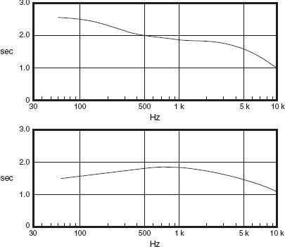
Figure 10.1:

Reverberation times of two famous concert halls in England.

The early decay time (EDT) is usually expressed as the time taken to decay by 60 dB, but extrapolated from a straight line drawn through the – 5 dB and –15 dB points. Alternatively, it can be calculated by taking the time from the 0 to–10 dB levels and multiplying the figure by six. If the resultant figure is greater than the actual T₆₀, then the early decay time is slower than the average decay time, and vice versa. Measurements made in this way are often referred to as RT₁₀, even though the resultant figure is that of the time for the sound to decay to 60 dB. In a reverberant room with a uniform decay rate, the two figures would coincide. The measurement is conventionally performed in octave bands. The concept is shown graphically in Figure 10.4.

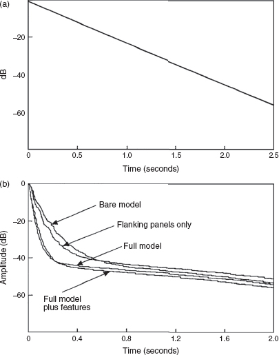
Figure 10.2:

Schroeder plots: (a) In a perfectly reverberant room, the Schroeder plot would show a straight-line decay. In the case depicted here, the RT₆₀ is slightly over 2.5 s; (b) This Schroeder plot of a test room shows how the installation of acoustic control items removes the energy from the early part of the decay curve, ‘cleaning up’ the room.

In small rooms, the truly diffuse sound-field required to produce reverberation can never develop, but the relative energy in the modes, discrete reflexions and diffused sound all contribute to the overall perceived sound. The Schroeder plots of Figures 10.2 and 10.3 show the overall envelope of the decaying energy, which is a very useful guide to the general behaviour of a room, but when problems exist it is sometimes necessary to see more detail.

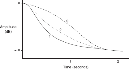
Figure 10.3:

Different decay characteristics.

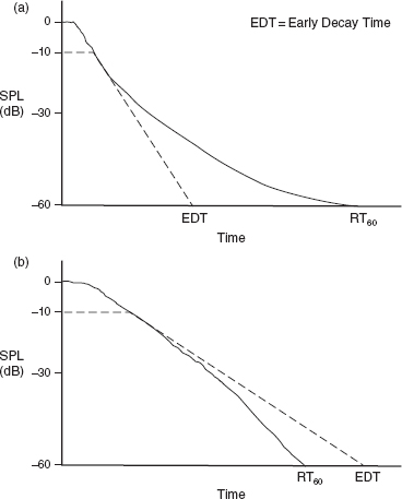
Figure 10.4:

(a) Early decay time shorter than RT₆₀; (b) Early decay time longer than RT_60.

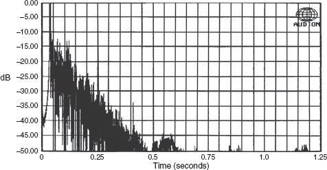
Figure 10.5:

Energy/time curve (ETC). This ETC is a representation of a room not too dissimilar from the bare model plot in Figure 10.2(b). The bumps at 0.55, 0.85 and 1.15 s were due to traffic noise. The plot was from an unfinished room.

Figure 10.5 shows an energy/time curve (ETC) in which the individual predominant reflexions can be seen as spikes, above the general curve of the overall envelope. These plots are, like the Schroeder plots, showing level against time, so the time between the initial event and any problem reflexions can be determined. When the time of travel is known, the path from the sound source to the microphone can be calculated. Any offending surface can then be located, and if necessary dealt with.

10.1.1 The Envelope of the Impulse Response and Reverberation Time

Despite the Schroeder plots and the ETCs both being representations of energy versus time, they each have their distinct uses. They are also generated in different ways in order to highlight best the aspects of the responses of which they are intended to facilitate the assessment. Figure 10.6 shows the impulse response of a room, which is a simple representation of sound pressure against time. It may at first seem plausible that half of this plot could be ‘smoothed’ to give a representation of the decay of the room, but it will be noticed that the plot is not symmetrical about its horizontal axis. It will also be noticed that there are many crossings of the horizontal axis, where the representation of the sound pressure level is zero. If we simply summed the two halves, or folded up the lower half of the plot on top of the upper half, then the zero-crossings, such as are indicated at points X, Y and Z on Figure 10.6(b), would retain their zero values. However, on listening to the decay of a room, it soon becomes intuitively obvious that the energy decay does not alternate between rapid bursts of energy separated by points of zero energy, but that energy is present in the room from the inception of the sound until its decay to below audibility.

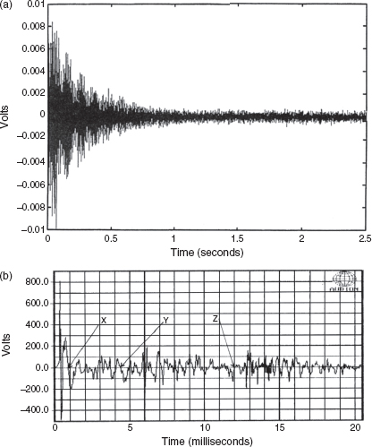
Figure 10.6:

(a) and (b). Impulse response of room (bare model) shown in Figure 10.2(b). (a) The impulse response shown here does not appear on first glance to relate directly to the more intuitively apparent presentation of the Schroeder plot of Figure 10.2(b), though both were generated from the selfsame measurement. The asymmetry of the upper and lower halves of the plot can clearly be seen, but due to the long time-window, the zero crossings are not obvious. (b) When the time scale of an impulse response is stretched (in this case the time scale is only 20 ms) the multiple crossings of the zero amplitude line can clearly be seen, such as at points X, Y and Z, and many other points.

For this reason, some integration is necessary if the simple instantaneous sound pressure representation of the impulse response is to be made into a better representation of energy decay. The impulse response shows only pressure against time, but, as shown in Figure 4.10, in reality the acoustic energy is constantly changing between the pressure and the velocity components.

A measure of the power, or energy per unit time, in such a signal can be calculated by squaring the signal and then averaging it, over a suitable length of time, to yield the mean-square value of the signal (the familiar rms [root-mean-square] value is the square root of this). The mean-square is a continuous positive value, which is only zero if the signal is zero for longer than the averaging time, and thus it does not contain the multiple zero-crossings present in the original signal. Provided the averaging time is long enough, continuous signals, such as a sine wave, have a mean-square value which is independent of time and independent of the length of the averaging time. However, estimates of the changing mean-square value of a transient signal, such as an impulse response, can be very dependent upon the length of the averaging time.

10.1.2 Schroeder Plots

In the early 1960s, Manfred Schroeder¹ had been frustrated in his attempts to accurately measure the reverberation time of some large concert halls. He was having trouble achieving repeatability in his results because, dependent upon the precise phase relationship of the elements within the random excitation noise, and the beating between the different modal frequencies thus excited, he could get some very different readings which could even halve, or double, on subsequent measurements. Confidence in such measurements was therefore not good. The method that he developed to overcome these problems involved the excitation of the room by a filtered tone burst, and the recording of the signal onto a magnetic tape recorder. The tape was then replayed backwards, and the output was squared and integrated by means of a resistor/capacitor integrating network. The voltage on the capacitor would then represent (in reversed time) the averaged energy decay of the room. Because the squared tone burst response is a positive function of time, its integral is a monotonically decreasing function of time. The resultant plot is therefore a gradually falling line, free of the up and down irregularities of many other decay time representations, and is thus easier to use for accurate decay time rate assessments.

Nowadays, the generation of Schroeder plots is usually by means of digital computers, which have made redundant the need for the cumbersome use of tape recorders in the making of these measurements. The use of Schroeder plots is widespread, because they show, perhaps more clearly than any other decay time representation, the presence of multiple slopes within a complex decay tail. It is now widely appreciated that the initial slope, for the first 10 dB of decay, is perhaps one of the most important characteristics in the subjective assessment of the performance of a room.

The decay curve for a Schroeder plot is derived by squaring the decaying signal and integrating backwards in time from the point when the response exceeds the noise floor (t₁), back to the start of the response (t₀). The value of the decay curve at any point in time (t) is therefore the integral of the response over the interval from t to t₁. The resultant decay curve is a smoothly varying, and (necessarily) monotonically decreasing function of time. This characteristic is a necessary condition of the total sound energy in a system (such as a room) after the source of energy has ceased. The technique is thus valuable in determining the decay slopes, particularly in the early part of the response, which are necessary for reverberation time estimates in conditions where background noise does not allow measurement down to –60 dB. However, any fine detail in the impulse response is lost, due to the time integration, so the Schroeder plots cannot show the individual reflexions which can be seen on an ETC.

For anybody unfamiliar with the term ‘monotonic’, it means either forever rising, or forever falling, although fluctuations in the rate of rise or fall can be allowed. The monotonically falling characteristic of the Schroeder plot decay curve is easy to appreciate, as once the energy source has been turned off, the absorption in the room can only lead to a gradually reducing net energy level in the decay tail (because energy cannot reappear once it has been absorbed).

10.1.3 Energy/Time Curves

The energy/time curve (ETC) is the result of applying a technique to a transient signal which does not depend upon time averaging, but which yields an estimate of a mean-square-like value, which varies with time. The seminal paper on this technique was written by the late Richard Heyser and was published in 1971.² As previously mentioned, the multiple zero-crossings of the impulse response do not represent points of zero energy. Before we look in more detail at the generation of an ETC, perhaps we had first better look again at the pendulum analogy, in order to understand why an instantaneously zero SPL is not necessarily representative of zero energy.

When the pendulum is at either end of its swing, it is at its maximum height but has zero velocity. When the pendulum is at the bottom of its swing, it has minimum height but maximum velocity. The two forms of energy present in the pendulum are potential energy, which is a function of the height of the pendulum above equilibrium, and kinetic energy, which is a function of the velocity of the pendulum. As the pendulum swings, there is an alternating transfer of energy from potential to kinetic to potential, with one form of energy being a maximum when the other is a minimum. The total energy in the pendulum at any time is the sum of the potential and kinetic energies, and is independent of time unless the pendulum slows down. A graph of either the height of the pendulum or its velocity would show multiple zero-crossings, and would not therefore be a measure of the total energy in the pendulum. One could, however, obtain a good estimate of the total energy by comparing one graph with the other, or even estimating one from the other, then calculating the two energies and summing them. The latter method is the basis for the ETC calculations.

A signal, such as the impulse response of a room, is treated as though it represents one form of energy in an oscillatory system, such as the pendulum. Using powerful signal processing techniques, such as the Hilbert Transform, it is possible to derive a second signal which represents the other form of energy. The two signals are similar, but ‘appear’ to be 90° out of phase with each other, as shown in Figure 4.9(b). One has a maximum or minimum when the other has a zero-crossing, and vice versa. The ETC results from squaring these two signals and adding them together.

The ETC does not rely upon time averaging (or integration) and therefore, to such an extent that the time response of the filters allows, does not mask any fine detail in the instantaneous energy of the signal. In general, the ETC of an impulse response has a characteristic which can increase as well as decrease with increasing time (it is not monotonic), and is thus useful for identifying early reflexions and echoes.

To summarise, the Schroeder plot is most suitable for reverberation time estimation where the main point of interest is the rate of decay of the energy in a room. The ETC is better for identifying distinct reflexions, or other time-related details of a specific impulse response, such as those generated by a loudspeaker system.

10.1.4 Waterfall Plots

Some of the characteristics of the ETCs and the more conventional T₆₀ plots can be combined into what is commonly known as the ‘waterfall plot’. Normally computer generated, these plots show a perspective view in a three-axis form, as shown in Figure 10.7. The vertical axis represents the amplitude of the sound, and the two horizontal axes represent time and frequency. Such plots are very useful, but care should be taken when assessing them. On first impressions it often seems that they contain all the values represented by the three axes, but the nature of their perspective representation can hide some details in ‘valleys’ which lie behind some of the ‘hills’. Nevertheless, waterfall plots are very useful forms of analysis, as in a single plot they allow an ‘at a glance’ assessment of reverberation time against frequency, and decay rates at different levels and frequencies. They not only have the ability to show discrete resonances, but also the ability to show the predominant frequency bands inherent within any individual reflexions. Despite all of this information though, one must always remember that what a room sounds like can still not accurately be assessed from any piece of paper, because measurement microphones, no matter how sophisticated, are not ears, and neither are they connected to human brains.

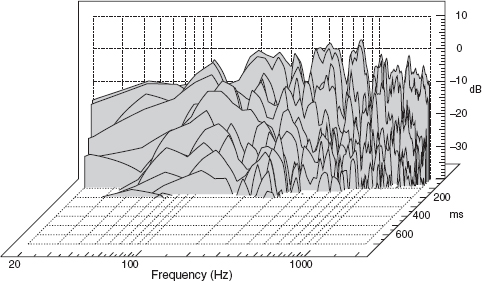
Figure 10.7:

This waterfall plot is of the finished control room described in Appendix 1. The cumulative spectral decay is represented in a three-axis format, the vertical axis representing amplitude, the front/back axis representing time, and the left/right axis representing frequency. In the case shown, only the low frequency range was being studied.

10.1.5 Directional Effects

Unfortunately, even when supplied with the RT₆₀ information about a room, and the Schroeder plots, and the ETC details, and the waterfall plots, this still tells us nothing about the diffusion or diffraction effects which may be taking place within the curves. We would still know little about any directional effects, which audibly may make one seemingly objectively innocuous reflexion more subjectively objectionable than an obviously higher-level reflexion approaching the microphone position (or listening position) from a direction which causes only little offence to the ear. Floor reflexions, for example, can be collected by a measuring microphone at a high level, yet our sensitivity to vertical reflexions, in general, is far less than to horizontal ones of the same intensity. Human beings have poor vertical sound discrimination, as our vertical position is usually known, and evolution has caused the development of horizontal discrimination at a more urgent pace. The knowledge of the proximity and direction of predators or prey have been great survival advantages. Because humans, their predators and their prey have historically largely been confined to living on the ground, two-dimensional horizontal localisation has been much more important than vertical localisation.

Another directional effect that is very difficult to demonstrate in overall response plots is the effect of any coupling between acoustic modes and structural modes. Any surfaces immersed in an acoustic energy field will, to some degree or another, vibrate because of the coupling to the acoustic energy. Sections of the structure of a room, or panels attached to the surface of the room, may vibrate and re-radiate energy into the room. The re-radiation will not only modify the modal interference patterns of the room, but will also act as a secondary sound source. To a person in the room its effect may well be audible, and detectable from a definite direction. This is another subjectively undesirable possibility that would be difficult to locate in most visual representations of room responses. It will no doubt by now be realised that if we wish to find out how a proposed room may sound, in advance of its construction, simply building to some preconceived specifications will obviously not suffice. If we need to know how a room may sound, we need to resort to other techniques.

10.2 Scale Models

Short of building full-size prototype rooms, the next best possibility would seem to be to build and test scale models. At concert hall level this is a proven method, at least as far as the major characteristics of the room are concerned. In a one-tenth scale model of a studio room, music can be played through miniature loudspeakers in the model room, speeded up by ten times, and recorded via miniature microphones placed in the ears of a one-tenth scale head. The sounds can be recorded, and then slowed down by ten times, and the result heard on headphones should be a reasonable representation of what the full-scale room would sound like. The above description of the technique is something of a simplification of the whole process, but the technique is useful and is used on some large-scale projects. One-fiftieth scale modelling is also used for larger halls, but because the frequencies must be scaled up by the same amount, air absorption losses are such that dry nitrogen is frequently used to fill the models, and in many cases, predictions are restricted to the low frequency range of the final, full-scale room. However, with rooms of studio size, the scale-modelling method would be expensive to put into operation. Furthermore, as the characteristics of acoustically small rooms are so dominated by surface features, which will not easily scale, the scale-modelling technique is likely to fail. Whilst frequencies, sizes and general modal responses can be scaled, the effects of absorbent treatments, the irregular surfaces of stonework, or the effects of floor resonances cannot be scaled. Mineral wool is almost impossible to scale, as are carpets or curtains. Scale models of small rooms can only be used to determine gross effects, and if effects are gross, they can normally be deduced from pure theory.

10.3 Computer Models

The power of computer modelling seems to increase day by day, but computers still cannot design rooms. They can be an aid to the experienced designer, who knows what he or she is looking for, but there is always a danger that in less experienced hands the graphics and apparent simplicity of the operation of the programs can lead to a belief that they give all the answers. They do not; the underlying rules and calculations behind the programs must be understood if gross over-simplification and over-confidence in the results are to be avoided. In many cases, exact solutions are only possible for simple shapes, whereas in practice, the same things that cause problems in the scaling of physical models will cause similar problems with computer modelling. Lack of ability to deal with the surface irregularities of different types of stone is one example of this general failing.

Computer models can be very useful as an interface between acousticians and any clients who do not have a good grasp of theoretical acoustics. The graphics can be used to explain to a client what a proposed room could look like, or to highlight the problems, which may be caused by an inappropriate choice of shape, size, or room features. There is always a danger, though, that in this world where computers are seen by many as essential tools for just about everything, the over-reliance on computer graphics and predictions will lead to a belief that it will achieve something that it will not. There are just so many parameters which contribute to the subjective character of a room; and not enough is known about their interrelationships to be able to program fully a computer sufficiently to give accurate predictions.

What follows are some words of the late Ted Uzzle, from a presentation which he made to the 72nd Convention of the Audio Engineering Society in Anaheim, California, in 1982. They are worth repeating here, as they do help to put the design process in perspective; ‘No sound system, no sound product, no acoustic environment can be designed by a calculator. Nor a computer, nor a cardboard slide-rule, nor a Ouija board. There are no step-by-step instructions a technician can follow; that is like Isaac Newton going to the library and asking for a book on gravity. Design work can only be done by designers, each with his own hierarchy of priorities and criteria. His three most important tools are knowledge, experience and good judgement.’ Ted Uzzle, incidentally, was not anti-computerisation; in fact, his presentation was on the progress of computerised design. In the almost 30 years separating then and 2011, there have been huge developments in the programs for computer-aided design, but still his words hold true. We still do not know enough about subjective acoustics to effectively program computers for design, and that is why many ‘design’ software packages are referred to as CAD – computer aided design. In many ways, it is what we do not know which can make acoustic design work so fascinating. There is still so much to be learned.

As stated in earlier chapters, the music recording rooms are extensions of the musical instruments; just as a guitar amplifier is an extension of the electric guitar. Studio rooms are not like control rooms. Not only are they usually allowed to have a sound of their own, but also they may be desired to have a sound of their own. In such cases, the design of a room is very much like the design of a musical instrument, and just as no computer program has yet, from within itself, come up with the design for a violin to equal the sound of a Stradivarius, nor can computers yet design musical rooms. Stradivari was a structural engineer as well as a musical instrument builder. His in-depth knowledge of the stresses and loading which his designs would demand allowed him to choose the appropriate thicknesses and cuts of the wood that were very close to their loading limits. It is such in-depth knowledge of the small details of processes which lead to refined designs.

Another drawback with computers is that one cannot have a conversation with them over dinner. So much of the work of a designer is involved with getting a feel from the client about the required characteristics of a proposed studio. Very frequently, prospective studio owners will only have a limited knowledge of the options available, and may not be able to articulate fully their wishes. In fact, many of their wishes may be based more on misguided beliefs or intuition rather than fact. Part of the job of a studio designer is to hold detailed discussions with the studio owners, offering options which may not have been considered, or relating anecdotes which may help them to understand points more clearly. In turn, the designer hears of the needs, the problems, the frustrations and the successes of the studio owners, and these shared experiences help to build up the designer’s own store of practical experience, which may serve in the future to forewarn of problems or to reinforce other experiences.

This appears to be one great failing of the typical Internet services offered, such as ‘send us the plans of your building, and for $X we will send to you an advanced studio design, the product of the very latest acoustic design technology’, and so forth. There is no attempt to discuss the client’s wants or needs. There is no personalised service, no meeting of minds, and no ‘heart’ in the process. It could be that people providing many such services do a great disservice to the whole acoustic design industry, and actually mislead many clients who fail to realise the limitations of the computer ‘designs’ that are being offered to them. In this technical age, however, the claims for computer designs can be deceptively seductive; but beware the pitfalls.

In a somewhat back-to-front way, though, the advancement of computer modelling has very much increased the total body of acoustic understanding. Rather ironically, this has not all come from the results of the computer analyses, but from the great stimulation which the need for programming information has given to basic acoustic research. In order to make a computer program, a great number of facts and figures are necessary. Without a rigorously factual input, a computer cannot produce a factual output. In recent years, the need for more programming information has provided both the need and the funding for further basic scientific work, and this has been a great boon to the whole science of acoustics and its applied technology. In turn, due to their great analytical capability and the speed of their calculations, computers have fed back a great deal of additional information, and have brought new people into the world of acoustics who otherwise would not have taken up this obscure science. With acoustics, there is always so much more to know. In fact, the application of computers to acoustic design is rather like their application to the production of this book. Except for the photographs, all the figures in the book were produced by computers, some were even generated by computers, but they were all conceived by human brains.

10.4 Sound Pulse Modelling

Some of the earliest attempts to ‘see’ what sound was doing involved shining light beams on to mirrors fitted to resonating tuning forks, and projecting the reflexions on to a screen as the tuning fork was rotated. In the days before oscilloscopes, this was one of the only ways to ‘see’ sine waves. To see what was happening inside models of buildings, light was also used in the technique of sound pulse photography, as used by Sabine in 1912. The principle goes back to 1864 when Teopler showed that when parallel light rays cross a sound-field at 90° to that of the ‘sound rays’, the part of the sound wave-front that is met tangentially by the light rays produces two visible lines, one light, the other dark, on a projection screen behind the sound-field. In the case of ‘sound pulse photography’, a spark is used as an impulsive sound source, and a second spark illuminates the model room, which is exposed to a photographic screen. The screen is shielded from the direct flash from the spark in order to prevent it from washing out the faint, refracted image. The images travel along the photographic screen at the speed of sound, and they can be sufficiently sharp to allow 1 mm wavefronts to be clearly perceived. Accurate representations of sound diffraction and diffuse reflexions can be observed, even in very small models. The progress of sound waves at different instants can be studied by altering the time intervals between the two sparks.

10.5 Light Ray Modelling

Light ray models have also been used in room analysis. In these cases, mirrors were used in the models in the places where acoustically reflective surfaces were to be situated in real life. Absorbent surfaces were represented by matt black painted surfaces. This technique was mainly used when there was interest in the effects of how particular reflective surfaces in the rooms could affect any parts of the modelled room where the principle reflexions would reach. By moving the light source(s) around to all the locations of interest, the distribution of complex reflexions from an entire surface could be studied. The main limitation to this type of technique as a design tool is that the wavelengths involved bear no resemblance to the actual wavelengths of the sound in the room under study. The diffuse reflexion and diffraction expected with low frequency sound waves therefore cannot be evaluated by this process. The technique only makes possible a reasonable estimate of the behaviour of sound waves at high frequencies.

10.6 Ripple Tank Modelling

Another modelling technique is the use of water trays, into which are inserted profiles of the room under investigation. A simulated ‘sound’ can be generated by allowing a drop of water to fall into the tank in an appropriate position, and the progress of the wave can be seen by watching the ripples cross the surface of the water. The model has the advantage that the slow progress of water ripples can make the wave propagation clearly visible, but there is the drawback that the model only operates in a two-dimensional plane. Ripple tank models are usually carried out in a glass-bottomed tank, illuminated from below by plane-parallel light rays. This method is excellent for demonstrations and is easily photographed. By selecting a depth of water of around 8 mm, the effects of gravity and surface tension can be effectively nullified such that long and short wavelengths travel at more or less equal speeds, just as they do in acoustic waves. Water wave models were used by Scott Russell for acoustical investigations as far back as 1843.

10.7 Measurement of Absorption Coefficients

Of course, design predictions cannot be well-achieved if the input data is erroneous. Care must be taken when using published absorption coefficients in calculations because the figures are generally only approximations measured under standard test conditions, whereas real applications will depend very much on things such as batch to batch similarity and mounting conditions. What is more, the very measurement systems, themselves, are fallible, so any coefficients measured by such systems cannot be definitive.

The traditional method of using a reverberation chamber places a sample of at least 10 m² in a room of long reverberation time and with nearly uniform distribution of very low wall absorption (usually hard, shiny walls). The empty room is first calibrated by measuring the spacially averaged reverberation time in one-third octave bands. The measurement is then repeated with the sample of absorbent material suitably placed in the room, and the absorption coefficient is calculated from the reduction in the reverberation time. However, despite the time-honoured nature of the technique, it is known to be unreliable because the conditions assumed in the reverberation time calculation depend on a well-distributed absorption, so by putting all the absorbent material in one place the statistically random incidence of all the reflexion paths is seriously disturbed. Unfortunately, the wide distribution of smaller samples would give rise to many more absorbent edges of the material, which would change the amount of surface area exposed to random incidence waves, and the diffraction produced by the edges of the material could also augment the measured absorption. Also, the effect of small patches of distributed material would be negligible at low frequencies, where their sizes were small compared to the wavelengths.

Perhaps, a more accurate measurement can be made in a plane-wave tube, but small measuring tubes cannot accommodate samples where the material is not relatively uniform on a small scale, or where a small sample may not be representative of the normal conditions of application. Such would be the case with a wall panel, where the overall absorption when mounted could not be assessed from a small sample. There are in situ measurement techniques for large, constructed surfaces, but they are complex, require much care and precision, and are also prone to being disturbed by other room effects such as spurious reflexions. Figure 10.8, taken from Acoustic Absorbers and Diffusers, by Cox and D’Antonio,³ shows a comparison of absorption coefficients for a single sample as measured in 24 different laboratories. In some cases, the differences are almost by a margin of 0.4, which on a 0 to 1 scale can hardly be considered to be trivial! The ‘impossible’ values above 1 (perfect absorption) show the effects of the diffraction and edge problems mentioned in the previous paragraph.

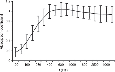
Figure 10.8:

Comparison of measured absorption coefficients for a single sample in 24 laboratories. The mean absorption coefficient across all laboratories is shown, along with error bars indicating the 95% confidence in any one laboratory measurement.

The thing to be most wary of is that absorbent materials measured under standard conditions may not perform in a similar way under different mounting conditions, and measurement under the precise mounting conditions used may not be either simple or reliable. Many acoustic design services offered on the Internet, for example, are based on calculations using standard absorption and diffusion figures, very little modified (if at all) with regard to their actual conditions of use. One cannot therefore consider such services as anything much more than generalisations.

In fact, even the reverberation times, themselves, are not always consistent when measured by different techniques. Schroeder’s frustration with reverberation time measurements was mentioned in Section 10.1.2. Fifty years later, the two plots shown in Figure 10.9 show the decay time of a film dubbing theatre, one measurement made by an engineer from Dolby Laboratories in England, and the other by a scientist at the prestigious Institute of Sound and Vibration Research (ISVR), one of the world’s leading acoustics research institutes; again in England. One measurement was made from a dual-channel FFT analysis and the other with a dedicated RT analyser. The starting conditions were good, with well over 50 dB of signal-to-noise ratio.

Especially with very low decay times, the options as to exactly how to go about the analysis are considerable. In these days, where almost every enthusiastic amateur has a program which they ‘know’ is absolutely accurate, how come we have the differences shown in Figure 10.9? The people who made the analyses were experienced professionals in very respected laboratories. It really cannot be the case that the enthusiastic amateurs know better, so in fact it must be concluded that it is difficult to have 100% confidence in decay time measurements, just as Schroeder noted in the early 1960s. In Figure 10.9, the difference between the two plots in the 600 Hz to 1200 Hz range is significant.

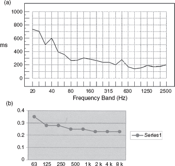
Figure 10.9:

Plot (a) shows the decay time characteristics of the dubbing (mixing) theatre shown in Figure 21.8, as analysed at the ISVR from a dual channel pink noise recording using an inverse Fourier transform and a reverse Schroeder integration; Plot (b) shows the decay time as measured by Dolby Laboratories using an AT5 reverberation-time analyser.

The differences between the plots shown in Figure 10.9 are partially due to Dolby working with ANSI (American National Standards Institute) recommended filters, and the measurements at the ISVR working to ‘best academic principles’. However, differences may also be due to the different systems making calculations which had been based on different concepts of where the slope should be measured from (there is no absolute rule for this). There are obvious advantages if people use standard filters for this process, such as the ANSI recommended filters, but standard filters need to be widely available and realisable in a wide range of measurement systems if everybody is going to make measurements which can easily compare with each other. On the other hand, in academic institutions, less easily derived filters and processing may be more definitively accurate, but their less simple realisation in a wide range of portable measurement systems may make room-to-room comparisons more difficult if different people have used different analysis techniques.

10.7.1 General Limitations to Precision

It is important to understand that there is no universally accepted technique for measuring the low frequency decay time in rooms with very short decays. It is perhaps worth quoting here something from the conclusion of an article by Philip J. Dickinson, first published in Acoustics Australia in 2005, then re-published in Acoustics Bulletin in 2007.⁴ ‘We can measure the light from a star millions of kilometres away, we can measure the time for light to travel a distance less than a tenth of a millimetre, we can measure the heat output of a candle more than a kilometre away – all to an accuracy of 3% or better – but we cannot measure a sound, even under strict laboratory control conditions, to better than ±26% (± 1dB in terms of percentage of power), or in the open air (it would seem) to much better than ±300% (±5 dB)’.

Much of the skill in many acoustic measurements is therefore in the interpretation of the results, not simply in the making of the measurements. This goes not only for reverberation (decay) time measurements, but also for absorption coefficient measurement and many others. Furthermore, even things which measure substantially similar may still sound very different to the ear. A very common error made by non-specialists in acoustics is to put too great a faith in absorption coefficients and reverberation/decay time figures. These are not things on which it is advisable to bet the family fortune on their veracity. It seems totally incredible when some mastering engineers write about the need to set their loudspeaker levels to be within 0.1 dB of each other, but perhaps they know something that the world’s greatest acoustic scientists have not yet discovered.

The problem also extends into sound isolation measurements between rooms. Let us imagine that we have two adjacent rooms in a studio: a live room and a dead room. How do we measure the realistic isolation? Where do we put the noise source? Where do we put the measuring microphone? What do we use as the noise source? All these variables can significantly affect the measured results. Let us imagine that we have a source in the live room and a microphone in the dead room. If we then swap them round, reciprocity demands that the isolation would be the same in either case. However, if we change the position of the source and/or the receiver, in either room, we will measure different results. The position of either the source or the receiver in the dead room will influence the results mainly in terms of distance from the live room, but little else. Conversely, the changing of the position of either the source or the receiver in the live room will change things more dramatically, depending on how they couple to the resonant modes. It is therefore difficult to give a client a precise figure for the inter-room isolation because if measured by standard techniques it may not represent the normal way in which the rooms are used.

In many countries there are regulations for the minimum isolation between classrooms in schools. In these cases, the classrooms are usually neither very live nor very dead, as the former would lead to intelligibility problems and the latter to having to use raised voices, which would be very fatiguing for the teachers. In these more ‘normal’ rooms there are standard ways to make the isolation measurements, based on experience of how to make them in a representative way. It is usually expected that a certain minimum of isolation when measured in the standard way will ensure that problems will not occur due to the noise from one classroom disturbing the concentration of the pupils in the adjacent classroom. However, such figures are not necessarily representative of the definitive isolation from one room to another. They are figures to meet legal requirements. In fact, if we changed the furnishings in either of the rooms, say from hard seats to soft sofas, we would probably increase the measured isolation between the rooms by reducing the ability of the room resonances to amplify the sound.

As mentioned in Section 3.10, legally, a problem could arise because a neighbour was receiving noise from an adjacent studio which was 1 dB over the permitted limit. Whether this figure was acted upon or not could depend on whether the person responsible for making the measurement considered that the studio or the neighbour had the greater credibility. It has been recognised that in the UK, around half of all complaints made about noise nuisance are actually motivated by reasons other than the noise, hoping that the noise nuisance, if proved, would lead to the closure of the place producing it, which the person(s) complaining primarily wanted closed for some other reason. Environmental noise officers often take this into account when making measurements. The imprecision of the measurement techniques allows some leeway, and gives the officials a margin for using their own judgement in dubious cases, although if a gross noise nuisance exists, the case would be clear.

The nonsense which exists on the Internet about many measurement concepts is monumental, and can be very misleading for the non-specialists. Acoustics deals with three-dimensional wave expansion, which cannot be fully described by reference to a couple of points in space – the measurement positions. As shown in Figure 10.8, not even the properties of the raw materials of construction can be relied upon to be accurately documented. It all depends on how the measurements are done.

10.8 Review

In computer models, the effects of all of the various physical modelling techniques can be incorporated into the programs, but nevertheless they are only analytical tools; just like the physical modelling methods. For achieving the best results from computer models it is essential that the users understand not only the limitations of the expressions, but also those of the mathematical models used by the programs. Unfortunately, this is rarely the case. There is some very heavy mathematics involved in these models, and there are a very limited number of individuals who understand fully the mathematical and the acoustical implications. These few people tend to reside in the academic world, and consequently may not be devoting their working lives to studio design. Neither will they necessarily have the practical design experience of professional designers. The whole team of specialists that it would take for a full understanding of many of the computer-derived implications is the sort of thing which could only be afforded by governments, and not by any normal prospective studio owners.

All modelling techniques are useful methods of scientific and technical investigation, and in computer form are very marketable items, with a ready multitude of customers wanting to buy them. However, one should never expect to glean more from the computer program than one knows how to interpret. The graphic displays are not gospel. They are perhaps more useful in locating problems than they are in suggesting what should be done about them. But that is generally true of the whole science/art of studio design, or, for that matter, the design of any room for musical performances. The previously quoted words from Ted Uzzle still hold very true, and are likely to do so for a very long time to come.

10.9 Summary

A great range of measurement techniques and their displays is needed in order to see many audible characteristics of a room. Each measurement technique has its strengths and weaknesses.

Schroeder plots show a good representation of the average energy decay, but lack detail within the curve.

ETCs clearly show individual reflexions, but only poorly demonstrate the curve of the decay.

RT₆₀ plots show time against frequency at the 60 dB level, but give no indication of what happens during the decay.

Waterfall plots show level against time and frequency, but cannot give any information about directional effects.

For the prediction of room responses, various forms of modelling can be used. Again, they all have their strengths and weaknesses, but they can be useful tools for investigating some specific areas of the performance of a proposed room design.

Beware of using published figures for absorbent materials too rigidly. The measurement techniques are not perfect, and even respected laboratories are not always consistent in their findings. Mounting and application conditions can also greatly affect the coefficients.

Reverberation/decay-time and isolation figures are also subject to considerable measurement error.

References

1 Schroeder, Manfred R., ‘New Method of Measuring Reverberation Time’, Journal of the Acoustical Society of 2 America, Vol. 37, pp. 409–12 (1965)

2 Heyser, Richard C., ‘Acoustical Measurements by Time Delay Spectrometry’, Journal of the Audio Engineering Society, Vol. 15, p. 370 (1967)

3 Cox, Trevor, J., D’Antonio, Peter, Acoustic Absorbers and Diffusers – Theory, Design and Application, Spon Press, London and New York (2004)

4 Dickinson, Philip, J., ‘Changes and Challenges in Environmental Noise Measurements’, Acoustics Bulletin, Vol. 32, No. 2, pp. 32–36 (March/April 2007)