CHAPTER 4

Room Acoustics and Means of Control

The main means by which we achieve the necessary sound isolation in recording rooms is by reflexion, because absorption, as a means of isolation, is rather disastrously inefficient. In typical isolation shells, the sounds produced within the rooms are reflected back from the boundaries, and thus contained within the space. Sounds emanating from without the room are similarly reflected back whence they came, and thus little sound can penetrate the isolation barrier from one side or the other.

Reflective isolation from exterior noises presents no problems, but this method of isolation to the exterior, by the concentration of the acoustic energy inside the room, means that in the extreme we are creating a reverberation chamber. This only serves to make the job of acoustically controlling the room much more difficult than it would have been in its less isolated original state, where much of the sound could leak out. This is especially so at low frequencies. In fact, one reason why so many domestic hi-fi systems sound better in people’s homes than the monitor systems in some badly designed control rooms has its roots in the relative degrees of isolation. Very often, the domestic constructions are of a much more leaky nature for low frequencies. Much of the energy escapes not only through the doors and windows but also through the structure of the buildings. This means that it is easier to achieve a more flat, controlled response in most domestic rooms than within the isolation shell of a simple control room, even though musical acoustics never enter the head of most domestic architects. If we start off with a highly reverberant shell, then the control measures must be much more drastic (and proportionally more expensive) than if we begin in a normal domestic room, where the reflected low frequencies are not so concentrated.

There is no doubt that once we provide a studio with a highly effective isolation shell, we are making our own lives much more difficult from the point of view of subsequent acoustic control. Nevertheless, the isolation is usually a prime requirement, without which the studio could not function effectively, so we have little option but to deal with the situation in which we find ourselves.

Figures 4.1 and 4.2 show a reverberation chamber and an anechoic chamber respectively. It is between these two acoustic extremes that all practical studio rooms are constructed. So by understanding the performance of these two extremes we will be able to get some feel for which characteristics of each of them we may require in our desired acoustics. First, however, we need to look at some basic wave acoustics.

There are many text books which wholly or partly dedicate themselves to a rigorous treatment of room acoustics. Some are listed in the Bibliography at the end of this chapter, and they are recommended reading for anybody wishing to take the mathematics and the theory some steps further. The purpose of this book, though, is to try to discuss these principles with people whose lives they affect every day, even if they do not have an academic background in acoustics or mathematics. For this reason the following discussion will be as accurate as can be achieved without the maths, but that does not imply that the mathematics would tell the whole story. In many of the situations that we encounter in room acoustics, there are simply too many variables, so in many cases a good feel for the problem is even more important than knowing the theory without having the practical experience. Anyhow, let us begin with a review of some basic acoustic principles.

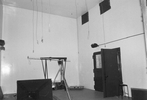
Figure 4.1:

The large reverberation chamber at the ISVR. It has a volume of 348 m³ with a reverberation time of 10 s at 250 Hz, and 5 s at 200 Hz. All surfaces are non-parallel and are made from painted concrete.

Figure 4.2:

The anechoic chamber previously shown in Figure 2.3, but here with almost all of its floor grids and supports removed, rendering it almost totally anechoic above its cut-off frequency.

4.1 Internal Expansion

When a sound source in a highly reverberant environment emits an acoustic wave, the wave initially expands according to normal free-field expansion.

Before the sound reaches the first boundary, the conditions are, by definition, anechoic. Therefore, let us first take the simple case of a loudspeaker emitting a low frequency sine wave in the region of a hypothetically perfectly reflective wall. The progressive wave expansion is shown in Figure 4.3. The situation for the listener, sat by the loudspeaker, would be absolutely identical if the situation shown in Figure 4.4 existed. In this case the wall has been replaced by a second loudspeaker, placed the same distance behind the position of the wall as that from the wall to the first loudspeaker. The two identical loudspeakers would be fed the same signal at the same level. Were the wall to have an absorption coefficient of 0.5, in which case it would absorb half the acoustic power, then this situation could still be identically mimicked by reducing the signal level to the second loudspeaker by 3 dB – half the power. Even if the wall were to have a frequency dependent absorption characteristic, as all real walls do have, the situation could still be identically replicated by means of an electrical filter having the same response as the wall absorption, in series with the feed to the second loudspeaker.

This leads us to the classic mirrored room analogy, as shown in Figure 4.5, when the behaviour of a sound source in a real room is visualised from the point of view of a listener sitting in a room with rigid walls and mirrors on all surfaces. Quite simply, from every point where a reflexion or a reflexion of a reflexion existed, the room would behave sonically as though there were no walls and an identical signal were being fed to all the ‘loudspeakers’ that were visible. It often seems to be easier for many people to grasp the concept of room behaviour in this way, because loudspeakers with volume and tone controls are much more familiar than the invisible concepts of frequency contoured acoustic reflexion. This analogy is useful because it is absolute. There are no differences whatsoever until we begin to introduce complex diffusive and scattering surfaces, but even then we could roughly visualise things by placing obstacles in the way of the reflexions or smearing the mirror with grease at certain points to make the reflected image more fuzzy.

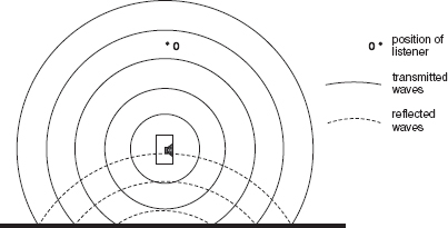
Figure 4.3:

When a loudspeaker is placed near to a solid boundary, some of the waves, which would have continued to expand in free space, will be reflected back from the boundary in the direction of the source and the listener. When the reflected waves arrive at the listener, and if the boundary is perfectly reflective, the situation and perceived sound would be identical to that shown in Figure 4.4.

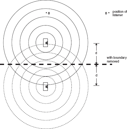
Figure 4.4:

The wave reflected from the boundary in Figure 4.3 can be represented by a loudspeaker placed behind the source loudspeaker with the boundary removed, positioned such that the second loudspeaker is the same distance behind the imaginary boundary as the source loudspeaker is in front of it.

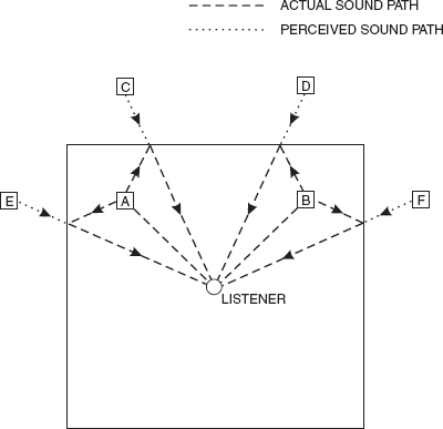
Figure 4.5:

Mirrored room analogy. Reflexions behave as if they were independent sound sources, located at the positions of their images. Floors and ceilings behave similarly: A and B, actual sound sources, C to F, apparent sound sources.

Let us now look at Figure 4.6, which encloses the loudspeaker within the four boundaries of a two dimensional room. In (a) and (b) the walls are anechoic, like the room shown in Figure 4.2, therefore they behave acoustically as though they do not exist and the loudspeaker is in free space. All that arrives at the points X are the direct waves from the loudspeakers. In (c) and (d) the walls are almost perfectly reflective, as in the room shown in Figure 4.1, which is a four-walled representation of the case shown in Figure 4.3. In this case the waves try to expand, but they are constrained by the perfectly reflective surfaces and so the paths of the waves continuously fold back on themselves. With nowhere for the energy to go, the wave pattern in the room rapidly becomes ultra-complicated, and the acoustic power within a hypothetically perfectly reflective room would build up until the room finally exploded. That is if it were hermetically sealed. In reality, of course, absorption exists, and even in the highly reverberant room shown in Figure 4.1 this acoustic energy drops by 60 dB in about 8 s. Figure 4.6(c) and (d) also show a further important point which relates very much to control room acoustics. If the loudspeaker is placed within the room, as opposed to being mounted flush within the boundary, it also sends low frequencies to the wall behind it, which then add to the reflexions in the room.

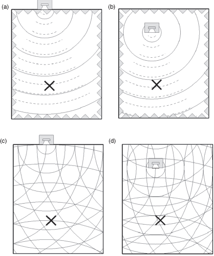
Figure 4.6:

Comparison of loudspeaker sitings in anechoic and reverberant spaces: (a) anechoic, flush; (b) anechoic, free-standing; (c) reverberant, flush and (d) reverberant, free-standing. At point X in the anechoic room, the low and high frequencies are perceived equally for both flush mounted and free-standing loudspeakers. However, in a more reverberant room, the low frequencies rapidly become confused. For the free-standing loudspeaker, the confusion sets in more rapidly than for the flush mounted loudspeaker in any given period. ____ omni-directional low frequencies; ----- directional high frequencies.

It can further be seen from Figure 4.6(c) and (d) that after the same period of time, the wave pattern is much more complex in the room with the free-standing loudspeakers than in the room in which they are flush mounted.

For steady-state signals, such as sine waves, the consequences of the room reflexions are frequency dependent. Figure 4.7 shows the pressure fluctuations in the air between a loudspeaker and a wall at three different frequencies. In the first case, the reflected wave arrives back at the source loudspeaker with a 90° phase shift relative to the direct wave. In the second case, there is an exact fit for two whole cycles between the source and the wall, so the reflected path corresponds exactly with the outgoing wave in terms of pressure and rarefaction peaks. In the third case, the reflected wave coincides exactly in anti-phase with the outgoing wave in terms of the relative pressure and rarefaction peaks. The sums of the wave pressures are shown in Figure 4.8 at two different positions. It can be seen that the effects at each position are quite different for the three frequencies shown.

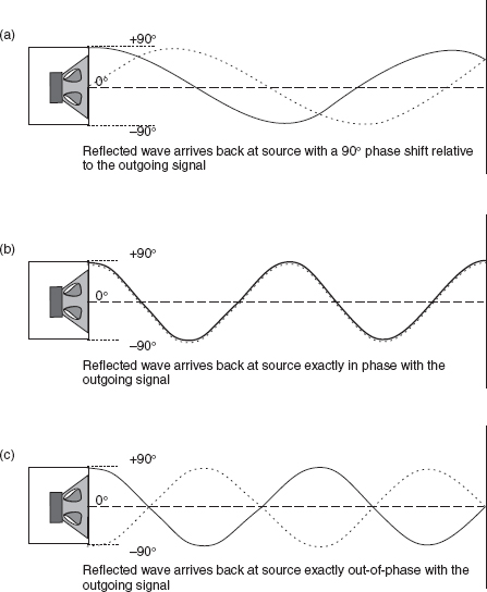
Figure 4.7:

Phase relationships of reflected waves at different frequencies.

This idea is shown in plan view in Chapter 11, in Figure 11.25 where different points in the room exhibit different responses to the combination of direct and reflected signals, dependent upon position and frequency. Whether this complex interaction of direct and reflected signals is a good thing or not is largely dependent upon whether we are listening to live music or to recorded music, and for what purpose. These concepts will be discussed later in their relative contexts. However, what we tend to want to avoid in almost all cases are the stationary waves, or ‘standing waves’ as they are commonly called. (See Glossary.)

Let us assume that the case of Figure 4.7(b) is modified with another wall behind the loudspeaker, at exactly the same distance from it as the front wall. It is shown diagrammatically in Figure 4.9(a). Because of the exact fit of four cycles across the room, and the position of the loudspeaker on the centre point, the first reflected wave will retrace exactly the path of the outgoing wave. The reflected wave from the rear wall will also retrace the same path, so the pressure changes will linearly superpose themselves, causing a build up in the wave motions.

However, there is another component of an acoustic wave besides that of the pressure. Figure 4.9(b) shows the velocity component of the wave motion, which it can be seen is shifted 90° from the pressure component. Thought of logically, this is reasonable enough, because when the wave which is travelling at the speed of sound strikes the perfectly reflective wall, it must obviously stop before returning in the reverse direction. For a stationary wave, the pressure component at a boundary must always be a maximum. This must be so, because with the velocity at zero, all the energy in the acoustic wave has to be carried in the pressure component: the energy simply cannot disappear every time the pressure change passes zero. There is therefore a continuous energy transfer, back and forth, between the pressure and velocity components of the wave.

To help to explain this, Figure 4.10 shows an analogous situation demonstrating the gradual energy transfers during the swinging of a pendulum. At either extreme of travel, the pendulum stops before retracing its path. This is akin to the wave particle velocity stopping as it reaches a reflective boundary, before being reflected in the reverse direction. When stopped, the pendulum has no kinetic energy, but with the height advantage over its vertically down position it has its maximum potential energy for its given distance of swing. At the low point of its travel, the pendulum passes through its point of maximum velocity, where its kinetic energy is at its maximum and its potential energy is at its minimum. (See Glossary, if necessary, for potential and kinetic energies.) At all points of the swing, other than the three already mentioned, the pendulum has a mixture of both potential and kinetic energy. Similarly, the wave motion has a mixture of potential and kinetic energy at all points other than its nodes and anti-nodes. The nodes are the zero crossing points on either the velocity or pressure plots in Figure 4.9. The anti-nodes are the positive and negative peaks in the plots, and it can be seen from (b) that the velocity nodes correspond with the pressure anti-nodes, and the pressure nodes with the velocity anti-nodes. The velocity and pressure are therefore always 90° out of phase with each other. The importance of this will become evident when, in later chapters, we begin to discuss the acoustic control of rooms.

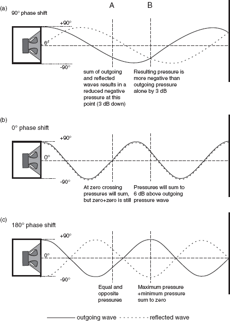
Figure 4.8:

Effects of phase shifts of reflected waves at different positions. Results of wave superposition (assuming that the wall at the right is perfectly reflective): (a) 90° (or 270°) phase shifts give rise to 3 dB variation in summed response. The resulting waveform would be a sine wave displaced to the right; (b) 0° phase shift results in the outgoing and reflected waves reinforcing each other at all points. The resulting waveform would be a sine wave of 6 dB greater amplitude; (c) 180° phase shift results in the outgoing and reflected waves cancelling at all points. The resulting waveform would be a flat line.

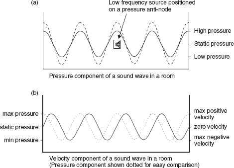
Figure 4.9:

Characteristics of a resonant mode: (a) At resonance, where an exact number of half-cycles can fit between the walls, the direct and reflected waves will superpose constructively to create a resonant build up, shown dashed; (b) The particle velocity component of the wave must always be at a maximum or minimum when the pressure component is at zero, in order to conserve the energy contained in the wave – see Figure 4.10.

4.2 Modes

The pathways available for a sound wave to travel around a room are known as modes, and in any room they are infinite in number. When an omni-directional sound source is in a room, it drives the room by radiating sound in all directions. If the sound source is then interrupted, some energy will be trapped in the repetitive pathways of the standing waves, indicated by the build up shown in Figure 4.9(a). The resonances associated with these pathways are called eigentones, which is German for the room’s ‘own frequencies’. These are the natural frequencies of resonance in the room. The non-resonant pathways which are driven by the sound source are known as forced modes. Those pathways which continue to decay for some time after the driving source has ceased are known as resonant modes. Thus, all modes are not standing wave paths, but all standing wave paths are modes. (See Glossary for more on modes.)

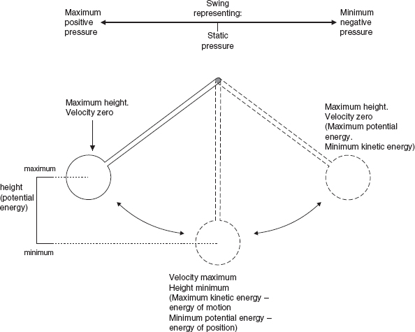
Figure 4.10:

Energy in a pendulum. At the points of maximum height there is a maximum of potential energy (the energy of position) but a minimum of kinetic energy (the energy of motion), [the latter because the pendulum must stop before it retraces its path]. At the place of minimum height, the pendulum is passing through its point of maximum velocity (and hence maximum kinetic energy). At all other places of its swing there is a continuous transfer of energy between potential and kinetic, and vice versa.

There are three types of resonant mode in a rectangular room. Axial modes, which exist between two parallel surfaces; tangential modes, which exist between four surfaces and travel parallel to the other two and oblique modes, whose pathways involve striking all six surfaces before returning to their point of origin to begin retracing the paths. In a room with all surfaces similarly treated, the axial modes of the longest dimension of the room tend to contain the most energy, because they strike fewer surfaces for any given distance travelled, and hence are absorbed less frequently. In real rooms, it is the absorption at the surfaces, on each reflexion, which depletes the energy in the modes. The lowest mode of the room will always be the axial mode between the two most widely spaced surfaces. Despite the longer total pathways for the tangential and oblique modes, their lowest frequencies will always be higher than the lowest axial mode, because it is the shorter side of the pathway which determines the lowest frequency to be supported in any resonant mode. This is because an exact integral number of half-wavelengths must fit into the dimensions of the tangential and oblique modes.

The typical pathways of the modes are shown in Figure 4.11. The combination of these three types of modes can form a very dense set of resonant frequencies in a reflective room. The following equation gives the frequencies of all the possible modes in a rectangular room

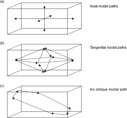
Figure 4.11:

Axial, tangential and oblique modes.

where:

x, y and z represent the number of half-wavelengths between the surfaces (up to the limit of interest – say the first 10 modes)

L = room length (m)

W = room width (m)

H = room height (m)

c = speed of sound (m/s)

For axial modes, only the x term is used; for tangential modes, the x and y terms are used, whilst for oblique modes the x, y and z terms are used.

The lowest axial mode exists at a frequency where half a wavelength fits exactly into the distance between the furthest two parallel surfaces. If the room is 15 m in length, for example, then the lowest resonant frequency would have a wavelength of 30 m, because two half-wavelengths would return the energy in phase to the starting point for the cycle to repeat. This would represent a frequency of about 11.5 Hz. The next mode would be at 23 Hz. These frequencies can be derived from the previous formula as:

but for axial modes, only, it can be simplified to:

The following axial mode would be at 34.5 Hz; the next at 46 Hz. On a linear frequency scale, the first 12 modes would appear as shown in Figure 4.12, but on a logarithmic scale, which more closely approximates to the way that we hear, they would be distributed as shown in Figure 4.13. Here, the increasing modal density per octave band can clearly be seen, and this is an important point, as we shall see later.

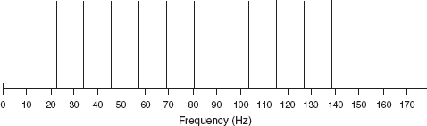
Figure 4.12:

The first axial modes of two room surfaces spaced 15 m apart, plotted on a linear frequency scale. Note the absolutely equal spacing.

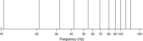
Figure 4.13:

The same modes as shown in Figure 4.12, but plotted here on a logarithmic frequency scale. The logarithmic scale relates better to the way in which we hear.

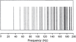
Figure 4.14:

The first 51 modes of a room. The first 51 resonance frequencies of a rectangular room of dimensions length = 4.7 m, width = 3.2 m, height = 2.5 m, plotted on a linear frequency scale. The modes at low frequencies are more widely spaced than those at higher frequencies, which make their perception as a form of colouration more likely. The thicker lines are where different modes are almost coincident in frequency. Not all of the 51 modes are well separated. Thirteen of them merge with other modes (after G. Adams).

Figure 4.14 shows the first 51 modes of a room of dimensions 4.7 m × 3.2 m × 2.5 m, also on a linear frequency scale. It shows how, in three dimensions, the modes definitely increase in number per unit bandwidth as the frequency rises. The problem which faces us is at the lowest frequencies, where the modes begin to separate. Figure 4.15(a) shows the same modes plotted to 100 Hz. The general ‘loudness’ of the room will be reinforced by the energy in the modes, and the overall perceived frequency response will be somewhat like the broken line which takes a roller-coaster ride across the modes and the spaces. It can clearly be seen that the room is perceived to have a flatter frequency response when the modes are more closely spaced. In Figure 4.15(b) exactly the same pattern exists, but the frequency scale this time represents a room where the dimensions have all been multiplied by three, to 14.1 m × 9.6 m × 7.5 m.

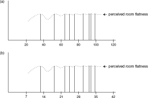
Figure 4.15:

Perceived responses in rooms with significant modal activity: (a) Room similar to that shown in Figure 4.14. A roller-coaster effect begins below 60 Hz; (b) Room of similar proportions, but with dimensions multiplied by three. Roller-coaster on-set is delayed until below 20 Hz. The modal pattern remains similar, and the perceived response shape also remains similar, but in (b) the frequency scale is reduced by a factor of three, yielding a smoother perceived response down to a lower frequency.

Two things are instantly obvious from the comparisons of the two figures. Firstly, that the modal pattern is exactly the same. This is because the modal pattern is a function of the shape of the room and its relative dimensions, not its absolute dimensions. Secondly, in the larger room, the flattest part of the roller-coaster response extends to a lower frequency. The implication of this latter point is that larger rooms with significant modal activity (i.e. they are reasonably acoustically reflective) will have responses which are perceived to be flatter down to a lower frequency than smaller rooms of the same shape. In reality though, the modal energy is not as represented in the previous figures inasmuch as the modes are not at spot frequencies and they do not all have uniform amplitude as represented by the height of the lines. In fact, they are more realistically represented as shown in Figure 4.16.

Figure 4.17 shows the measured power output from a loudspeaker, both in an anechoic chamber and in a room with considerable modal activity. The loading effect of the room which augments the low frequency response will be dealt with in later chapters, but it can be seen how, if the modal density is tightly packed and extended in frequency range, the room can have an overall frequency response which is acceptably flat. The effect of the modal activity is to make the room sound louder in response to whatever sound is being produced within it, compared with what would be perceived from the same sound source in an anechoic chamber. This is true whether the sound source is a loudspeaker, a cello, a tuba, a pipe organ or any other instrument that can provide a relatively continuous output. Things get a little trickier to explain when we come to impulsive sources and the musical transients from percussive instruments, but we will come to that later.

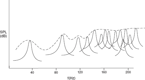
Figure 4.16:

Modal response of a typical room. The individual modes are shown with typical frequency spreading and different amplitudes. This is perhaps more representative of reality than Figure 4.14, which shows the modes as spot frequencies. A typical partially damped mode will be active for around 10 Hz either side of its nominal frequency.

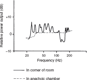
Figure 4.17:

Increase in loudness and extension of low frequency response by modal support. The measured power output of a closed-box loudspeaker system placed in the corner of a room (x = 0.7, y = 0.7, z = 0.5 m). The power output measured in an approximately free space (an anechoic chamber) is shown by the broken curve. The augmentation of the power output due to the room modes is clearly shown; as is a broad dip around 150 Hz due to the early reflexions.

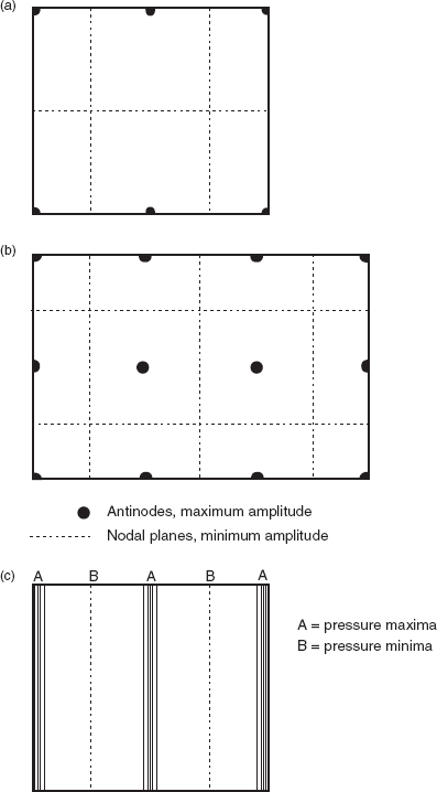
Nevertheless, in the low frequency range, where modal separation exists, the standing wave activity is usually undesirable, because the response of the room becomes heavily dependent upon the position of both the source and the receiver, be that a microphone or a listener. Figure 4.18 shows the spacial dependence of pressure distribution for two different types of mode. In (a) and (b) the pressure is high at the dots and low at the dashed lines. In (c), the pressure is high where the lines are packed close together, and lower elsewhere. This type of unevenness can be clearly heard when walking around any normal room in the presence of a low frequency tone. Figure 4.19 shows two alternative presentations of the same phenomenon. A conventional loudspeaker or musical instrument placed on a pressure anti-node would be capable of strongly building up a resonance if the output, or a portion of it, coincided with the resonant modal frequency. A listener on an anti-nodal point would also hear a strongly amplified sound. However, a monopole (but not dipole) loudspeaker or instrument placed on a node would not be able to drive the resonance, because the reflexions would constantly be returning to the point of origin out of phase with the drive signal, and so would tend to cancel it. Similarly, a listener on a nodal plane would hear little or nothing at the resonant frequency, even if the source were on an anti-node, because of the cancellation taking place on the nodal planes. Clearly this sort of spacially dependent distribution is not desirable, because it is also frequency dependent, so some notes intended to be equal in level would be perceived to be very different, depending upon where an instrument or listener was positioned and on the note being played. The effect is very easy to demonstrate by passing a low frequency tone through a loudspeaker in a reasonably reverberant room and then walking around the room and listening at different heights. The high and low pressure positions are easily audible, but their location will change as the frequency is changed.

4.2.1 The Summing of Modes and Reflexions

Figure 4.20 shows the gradual way in which a reflective room can upset the frequency balance of a sound source in response to a wideband signal, such as music or pink noise. In this case the source is non-centrally positioned in a rectangular reflective room, with the microphone placed some distance from it. Shown in Figure 4.20(a) is the anechoic output from the source, which is what exists, by definition, within the room in the short time until the effect of the first reflexion is noticed. The affect of the superposition of the first reflexion, from the floor, is shown in (b) and (c) to (f) show the cumulative build up of reflexions from each boundary in turn, until the whole room is contributing to the response. Moving the source around the room, whilst leaving the microphone in the same position, would change the pattern of (f), even though (a) would remain the same. In rooms for the playing of music, such variation can have the benefit of adding variety to the sounds, but in quality control listening rooms it is definitely not desirable, as a fixed reference is needed. The frequency and positional dependence of the modes is easily demonstrated by humming in a tiled bathroom with the towels and curtains removed.

If a room has two identical dimensions there will be augmentation of the energy at frequencies where the common dimensions apply. In the case of a cubic room there will be no difference in the axial modes for the three axes, therefore they will superpose themselves on each other and produce very strong resonances due to the common room dimensions. This will result in greater spaces between the modal frequencies, because there will be less frequency distribution than would be the case if the three dimensions were different. Common multiples of the axial distances can also reinforce and separate the higher modes. In a room 15 m × 10 m × 5 m, for example, the 5 m half-wavelength could fit into each dimension, and so could resonate strongly.

In an attempt to avoid such coincidences, many rooms intended for musical performance or reproduction have been designed with only non-parallel walls. In general, such approaches do not reduce the overall number of resonant modal pathways, or the overall number of coincident modes, but they do tend to have the ability to reduce the more energetic axial modes, and this can be an advantage in some circumstances. Unfortunately, the calculation of the modal frequencies in such rooms is too complex to be practicable, and no formulae exist, so such designs tend to rely very greatly on the experience of the designers.

4.3 Flutter Echoes and Transient Phenomena

Whilst on the subject of non-parallel walls, another advantage which they can offer is the avoidance of flutter echoes. These are the rapid repeats which can be heard when, for example, hands are clapped between two hard-surfaced, parallel walls. They usually exist, buried in the general reflective confusion, in all rooms with hard, parallel surfaces, but are usually most noticeable and objectionable when they are left exposed, such as when only two reflective surfaces exist. Such would be the case when a room with curtained walls had a hard surfaced floor and ceiling. Flutter echoes, per se, are normally only perceivable if there is a time interval of more than about 30 ms between the discrete repeats. With shorter time intervals, the ear tends to integrate the sound power to produce a continuous sound of greater loudness, but usually with a distinctly nasal or metallic ‘ring’. It is the regular, periodic nature of the repeats between a single pair of parallel surfaces which makes the flutter echoes or the ringing colouration so subjectively objectionable. Whenever encountered in a listening room they should be dealt with, either by means of absorption, by geometrical methods, or by diffusion. As a period of around 30 ms is necessary for a true flutter echo to be audible, it follows that a path length of much less than 8 or 10 m between the reflective surfaces will not exhibit the problem as a series of separate, perceivable echoes. What will predominate are the colourations in timbre due to the modal resonances that any impulsive stimulus excites.

Figure 4.18:

(a) Plan of the pressure distribution of a 2.1.0 tangential mode; (b) The distribution of the amplitude of the sound pressure throughout a room of a tangential 3.2.0 mode; (c) Pressure distribution of a single axial mode. Note how in (c) the wave is progressing across the room as a series of compressions and rarefactions. The progress of an acoustic wave (unlike the wave motion of light, which moves in the general fashion of a snake) moves somewhat like an earthworm. The worm moves in a straight line by means of the passage of a series of contractions and elongations through the length of its body. The use of sinusoidal graphs to represent a sound wave merely shows the level of the pressure distribution, and not its form. This is why light waves can be polarised. They have a lateral oscillation which can be reorientated, but sound waves cannot.

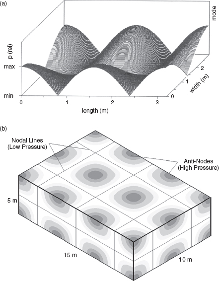
Figure 4.19:

(a) Representation of the sound pressure distribution in a rectangular room of the same tangential mode as depicted in Figure 4.18(a). The vertical axis is pressure. (b) A three-dimensional representation, this time for the 3.2.1 oblique mode at 58.9 Hz.

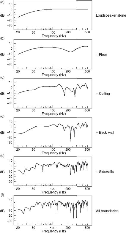
Figure 4.20:

Gradual build up of room reflexions and their effect on the overall response.

Unlike the precise reflected phase relationships which are necessary for resonant standing waves to build up, transient sounds do not exhibit phase shifts. Rather, with temporal displacements, they exhibit phase slopes, which represent the rate of change of phase with frequency. As a transient signal contains a great number of frequencies (and some, such as delta functions, contain all frequencies), each contributing frequency will have its own individual phase shift. Figure 4.21 shows a phase shift in a sine wave. The waveform itself has in no way been affected; the whole pattern has simply been shifted sideways. On a pure tone, such a shift has no audible effect. However, if these shifts are applied frequency by frequency to a transient signal, the results would be as shown in Figure 4.22 – a great change in the overall waveform. In fact, the behaviour of rooms to steady-state and impulsive (transient) sounds tends to be very different, and later we will address the question of how to simultaneously deal with these aspects of sound which require very different treatments.

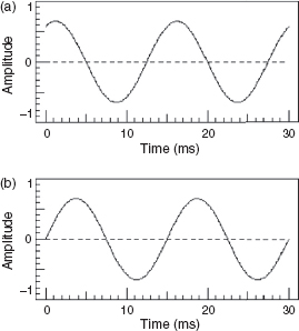
Figure 4.21:

Phase shift in a sine wave. With respect to the sine wave shown in (a), the sine wave in (b) is shifted by 90°. Nothing has changed except its position along the time axis. The quality and quantity of the wave are unaffected (shape, frequency and amplitude).

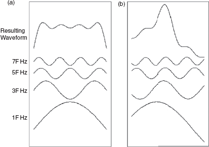
Figure 4.22:

Waveform change due to phase slope difference: (a) Shows a waveform broken down into its sine wave components; (b) Shows a totally different waveform, but consisting of exactly the same quantities of the same sine wave components. The only difference is that a phase slope has been applied, shifting the relative phases of the individual component frequencies.

4.4 Reverberation

Once we enter the realm of reflexions of reflexions of reflexions, and beyond, we are beginning to develop reverberation. Both the multiple repeats (echoes) of transient events and the modal build up of more steady-state sounds all contribute to the reverberant energy of a room. This consists of a hyper-complex sound field that is said to be statistically diffuse and to contain the same total energy in any given volume in any position in the room. In reality, such a purely diffuse sound field cannot exist. There must be a net flow of energy away from the source, because the sound radiates from the source. Furthermore, unless the reverberant room is extremely large, there will still be detectable modal activity at low frequencies. In the reverberation chamber shown in Figure 4.1, the field is only statistically diffuse down to around 150 Hz, below which spacial averaging must be performed. This can be done by taking the mean of measurements with the source and receiver in different positions.

Bear in mind, also, that if the chamber has a mean decay time of 8s, then the sound waves will have travelled 344 × 8 m, about 2.7 km, before they decay by 60 dB (344 m/s being the speed of sound in air at room temperature). This helps to give some idea of what is going on in a reverberant field. A further aid to visualisation is the concept of the mirrored room, once again, but with very reflective mirrors. In a room of such long reverberation time (RT₆₀ or T₆₀) the room surfaces would appear to be absolutely covered by images of loudspeakers, disappearing into infinity. This concept is also valid for time-varying signals, such as music. The smallest, most distant images would behave like the music originated from them at the same time as it emanated from the source in the room, but the furthest discernible tiny images of loudspeakers would be 2.7 km away, and the sound from them would arrive 60 dB down and 8 s later.

In a very reverberant room, the energy decay is exponential, which means that when it is plotted on a logarithmic scale the decay slope is a straight line.

4.4.1 Measuring Reverberation Time

The length of time that it takes for a sound to decay in a room is a function of the absorption of the surfaces and the distance between impacts with the room boundaries. The average distance that a sound will travel between each of the surfaces on its path to decay is known as the ‘mean free path’, which assumes all possible angles of incidence and position. In a reasonably rectangular room, the mean free path (in metres) is given by:

where:

MFP = mean free path (in meters)

V = room volume in m³

S = total surface area in m²

Note: MFP is often written L_AV (average length)

The time between surface contacts in any given room is given by:

which simply divides the former value by the speed of sound. (T = time between reflexions in seconds, and c = the speed of sound in metres per second.) It is worth noting here that there may, in certain rooms, be differences in the above path lengths and times, depending upon whether the reflexions are specular or diffuse, though for the purposes of this chapter it is a minor point.

There are numerous equations for the measurement of reverberation time because there is no universal equation which suits all circumstances. This is because the hypothetical perfectly diffuse field is never achieved in practice, so several ‘best fit’ approximations are available for different circumstances. (There is always a net flow away from the source.)

The oldest, and still very widely used equation, is the Sabine formula, named after Wallace Clement Sabine who pioneered reverberation time calculation. The Sabine formula is represented by the equation:

where:

(R)T₆₀ is the decay time (reverberation time) in seconds

V is the room volume in m³

S is the total surface in m²

0.161 is a measurement constant (there is a different constant for imperial measure, 0.049 in feet)

α is the mean absorption coefficient of the room.

This formula is really only valid for rooms of relatively low absorption, where α is less than about 0.3 (see Section 4.5), because it becomes increasingly inaccurate as the absorption increases. In fact, at the extreme, it predicts a reverberation time even when absorption is equal to 1. Perfect absorption (α = 1) could only be the case in a room with no walls, which therefore would not exist, so nor could the reverberation. Anyhow, if the total absorption coefficient is less than 0.3, the errors with this equation are less than 6%, which still renders it a valuable equation when used appropriately.

In recording studios, however, we are generally dealing with a much higher absorption coefficient. So high, in fact, that in some very highly absorbent control rooms the sound would decay by 60 dB before even having had time to strike each surface once! Remember that one of the assumptions about reverberation time calculations is that the sound energy visits all surfaces many times with equal probability. In highly absorbent rooms it is better to refer to the T60 as the decay time, rather than the reverberation time, because the decay really only consists of a short series of reflexions.

Another commonly used means for the calculation of reverberation time is the Norris–Eyring reverberation equation:

The minus before the 0.161 V is to restore the result to a positive value after the use of the natural logarithm (ln). The 1 – α term is derived from the fact that if perfect reflexion is taken as 1, then each time that a sound wave encounters a wall the reflected energy will be equal to 1 minus the energy absorbed by the boundary, which is represented by α, the absorption coefficient. Once again, though, this equation fails in the case of relatively high absorption.

It is perhaps worth noting here, whilst on the subject of reverberation, that as room size increases the reverberation time increases proportionately, even though the average absorption remains constant. This can be deduced from Equation 4.3, which has a term in cubic metres over a term in square metres, hence:

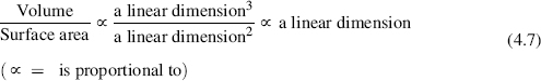
The net result is that as the linear dimensions increase, then so does the reverberation time if other factors remain constant.

It may seem a little strange that we have spoken so much about reverberation, merely to conclude that it is only marginally applicable to most recording studio rooms, and that the equations for calculating it are almost no use at all in any but the very largest of recording studios. Nevertheless, to know this is important, and the greater understanding of what constitutes reverberation is an important aspect of understanding room acoustics in general.

4.5 Absorption

The most important controlling factor in room acoustics is absorption. The coefficient of absorption is the proportion of the acoustic energy which is not reflected when an acoustic wave encounters a boundary. All boundaries absorb to some degree or other, which is why the concept of a perfectly reflective wall is purely hypothetical.

There are numerous means of absorbing acoustic energy, most of which result in converting it into heat. The possible exception is when absorption includes transmission, in which case the energy is lost to the outside world, such as via an open window, but eventually even this acoustic propagation will be absorbed in the air and converted into heat. At 1 kHz, the loss in dry air is about 1 dB per km, but in humid air it can be ten times that figure. Note that the 6 dB SPL reduction for each doubling of distance is not energy loss, but merely redistribution over a wider wavefront, as described in Section 2.3.

There are fibrous absorbers, porous absorbers, panel absorbers, membrane absorbers, Helmholtz absorbers, and these days, active absorbers, which will be mentioned in later chapters. They all function in their own ways. Some of them absorb by their action in arresting the particle velocity, in which case they need to be spaced away from the hard boundaries. Others act on the pressure component of an acoustic wave, in which case they need to be placed at the boundaries of a room.

The fibrous and porous absorbers can be considered together (fibrous absorbers are a sub-group of porous absorbers in general), as they both work by frictional losses caused by the interaction of the large internal surfaces of the material with the velocity component of the sound wave. Because the rapidity of the pressure changes (the pressure gradient) rises with frequency, the effectiveness of porous/fibrous absorbers also rises with frequency, due to the fact that the frictional losses increase as the particle velocity increases. As a result of this, the effect of these types of absorbers is affected by their density, their porosity, the space between the absorbent material and the wall, and their thickness. There are certain trade-offs, though. Table 4.1 shows the effects of thickness and density on fibrous absorbers. In general, barring any extra production processes that need to be paid for, one tends with most materials to pay for weight. Prices per kilogram are usually what count.

From Table 4.1 it can be seen that if we were to use a material such as 30 kg mineral wool, then at 125 Hz a thickness of one unit (say, 2.5 cm) would have an absorption coefficient of say 0.07, yet a thickness of 4 units (10 cm) of a similar density would have an absorption coefficient of 0.38 – over 500% greater for probably four times the price (four times the thickness of the same density = four times the weight). However, if we had our given piece of mineral wool of one thickness unit (2.5 cm), and an absorption coefficient of 0.07 at 125 Hz, and another piece of four times the density (four times the weight per given volume) but the same thickness, the absorption coefficient would only rise to 0.1. We would therefore be paying about four times the price for an improvement in absorption of less than 50%. Clearly, as we compress the mineral wool from 30 kg/m³ to 120 kg/m³, it becomes more compact, and there are fewer spaces between the fibres for the air to pass through. In the extreme it would become a solid block, with almost no air inside, and therefore would no longer be porous. In this state it would lose almost all of its ability to absorb.

Table 4.1: Effect of thickness and density on acoustic absorption

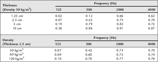
So, at 125 Hz, weight for weight, and hence in rough terms cost for cost, adding four layers of a lower density material and allowing it to occupy four times the space would produce over five times the absorption increase over a single piece. Compressing those four layers into the space of one would reduce the absorption by a factor of about 4. Note, though, in Table 4.1 how at higher mid frequencies, and above a certain minimum thickness, neither increasing the density nor the thickness has much effect.

4.5.1 Speed of Sound in Gases

In fact, whilst we are dealing with comparative tables, let us look at some of the mechanisms responsible for the effects shown in Table 4.1. Newton originally calculated the speed of sound in air from purely theoretical calculations involving its elasticity and density. He calculated it to be 279 m/s at 0°C, but later physical experiments showed this figure to be low, and that the true speed was around 332 m/s. There was conjecture that sound propagation only took time to pass through the spaces between the air particles, and that only the ‘solid’ particles transmitted the effect instantly. Newton rejected this, but then proposed that whilst the sound took a finite time to travel through the particles, the particles themselves did not occupy the entire space in which they existed, and that it was this fact which accounted for the difference. This idea also failed to be convincing. The difference continued to mystify people, until, in 1816, Pierre Simon, the Marquis de Laplace, applied what is now known as Laplace’s Correction.

It is now common knowledge that air heats when it is compressed, and cools when it is rarefied. As a sound wave travels through air, it does so in a succession of compressions and rarefactions, like an earthworm. As mentioned earlier, Newton’s calculations were based on the elasticity and density of the air. Elasticity is the ability to resist a bending force and to ‘push back’ against it, and the speed of sound through a material is partially dependent upon its elasticity. As the compressive portion of a sound wave compresses the air, it increases its elasticity in two ways; firstly by increasing its density and secondly by the heat which the compression generates. Where Newton had gone wrong was in the omission of the temperature changes from his calculations: he had only taken into account the elasticity increase from the density change. Perhaps this was due to the fact that there is no average temperature change as a sound wave passes through a body of air. However, locally, there are temperature changes in equal and opposite directions on each compression and rarefaction half-cycle. It is tempting to deduce that the increases and decreases of temperature would cancel each other out, which is perhaps exactly what Newton did, but they do not.

As air is compressed its volume is reduced, and on rarefaction its volume expands. The internal force which resists these changes in volume is its elasticity. If a tube containing air is sealed at one end and fitted with an air-tight plunger towards the other end, then as the plunger is pushed and pulled, the air will compress and expand. When the force on the plunger is released, it will spring back to its resting position. If the tube was then filled with a gas of higher elasticity, the force needing to be applied to the plunger for the same volume changes would be greater, as the higher elasticity would be more able to resist the changes.

It is possible to visualise the transmission of sound through air in a manner similar to that shown in Figure 4.23. In this figure, a series of heavy balls are seen contained in a tube, and separated by coil springs. If the springs are quite weak, then an impact applied to the left-hand side of ball A will pass to B, and on to C, and so forth, but there will be a noticeable delay in the transmission of energy from one ball to the next. The wave will clearly be seen to pass along the tube, as shown in Figure 4.24. Now let us assume that we apply heat to the springs, and the effect of the heat makes them much stiffer. Another impact applied to ball A will again pass down the tube, but with stiffer springs the wave will travel more rapidly.

Figure 4.23:

Energy transmission via masses and springs. Four balls A, B, C and D are separated by springs in a glass tube. The system is shown in equilibrium, with no force applied, and the springs in a relaxed state.

Figure 4.24:

Application of force to the system shown in Figure 4.23. If a force is applied to ball A, it will transmit energy to B via the spring. B will then transmit energy to C via the B–C spring, and so forth, until the whole chain of balls and springs is moved in the direction of the applied force. The speed with which the force will pass along the line is proportional to the stiffness of the springs (the elasticity of the coupling), and the mass of the balls. In the above example, the spring between A and B is seen to compress. The force on B is thus no longer in equilibrium, so B will move towards C, transferring some of the energy in spring A–B and compressing spring B–C until springs A–B and B–C are in equal compression. B will then tend to come to rest. In this state, spring B–C will be partially compressed, so C will have more compression in the B–C spring than in the C–D spring, and so will move in the direction of D. Due to the applied force and the momentum in the moving balls, the system will oscillate at its natural frequency until it finally comes to rest, shifted to the right, when all the applied energy has been expended.

In fact, at the extreme condition of almost rigid springs, the passage of the impact from ball to ball would be more or less instantaneous, as the ball/spring combination would behave similarly to a solid rod. The speed of the transmission of the force through the system can therefore be seen to be proportional to the stiffness of its springs. Effectively, in air, the particles can be thought of as balls being connected by springs, and the elasticity of the air is a function of the strength of these ‘springs’. The force on one air particle thus compresses the spring, heating it up, and hence increasing the elastic force which acts on the next particle. The heating effect caused by the compression thus serves to augment the elasticity of the gas, and hence the speed with which sound will propagate through it.

In the process of rarefaction, if we consider our tube to again contain coil springs and heavy balls, and if the balls are securely attached to the springs, then a rarefaction will pull on ball A, which will in turn pull on ball B, and on to the other balls in turn. At rest, the elastic force on ball B holds it in position, because the springs A–B and B–C are in equilibrium. By pulling ball A away from ball B, the elastic force on B is reduced on the side nearest to A, thus the greater force from spring B–C will begin to force B towards A, until equilibrium is restored. As B begins to travel towards A, the force B–C will become less, so in turn the extra force D–C will begin to push on C, which will begin to move towards B. The wave of energy will propagate along the tube until all the balls are equally spaced once again, but all shifted slightly further in the direction of the pulling force. This is where, somewhat surprisingly, we find that the cold of rarefaction serves not to cancel the heat of compression, but to work in concert with it by reducing the spring stiffness and aiding the rarefaction.

In rarefaction (in our analogy), the density of the A–B ‘spring’ is thus reduced, so the force on the C side of B will be greater than on the A side. The cooling produced by the rarefaction will then reduce the elasticity still further (weakening the spring) and thus will act in the same direction as the density reduction, making the A–B force even less. This will mean a greater differential between the A–B and B–C forces, so B will be pushed away from C with greater force than that of the rarefaction density change alone.

Hopefully it can be seen from the above discussion that the heat of compression and the cold of rarefaction both work in the same direction as the density changes, and hence both increase the effect. The additional help caused by the elasticity changes due to heat is the reason for the speed of sound in air being greater than that first calculated by Newton from the elasticity and density alone. The heat of compression and the cold of rarefaction do not cancel, but work together to increase the speed of sound through the air. Once this was realised, experiments were performed to test the ability of air to radiate heat, which was subsequently found to be very poor. This explained why the temperature changes remained in their respective compression and rarefaction cycles, and did not affect each other.

The reason for discussing all this history following the table of absorption coefficients of mineral wool at various densities and thicknesses is that the above fact is one of the mechanisms at work. In loosely packed fibrous material, such as mineral wool, glass fibre, bonded acetate fibre or Dacron (Dralon) fibre, the fibres can act to conduct the heat away from the compression waves, and release it into the rarefaction waves. This removes a great deal of the heat changes available for the augmentation of the elasticity changes, and hence tends to reduce the energy available for sound propagation. It changes the propagation from adiabatic (the alternate heating and cooling within the system) to isothermal, which slows down the speed of sound. It was the isothermal state that Newton had calculated, but it was the adiabatic state that was the normal situation. Due to the above effects, a loudspeaker cabinet which is optimally filled with fibrous absorbent material appears to be acoustically bigger than it is physically, as the speed of sound within the box is slowed down by the more isothermal nature of the propagation through the absorbent fibres. Fibrous absorbents can effectively increase the size of a loudspeaker cabinet by up to about 15%, but new activated carbon materials may be able to increase the effective volume by up to 50%.¹

Incidentally, Laplace’s correction, as referred to earlier, is quite easy to explain. If we place a known volume of air at 0°C, and at a known pressure, into a pressure vessel, then heat it by 1°C, the air cannot expand, so the pressure will rise. If we then place the same volume of air, also at 0°C, in a vessel of the same volume, but fit it with a plunger which can be forced outwards as we heat the air to 1°C, the pressure can be allowed to remain constant by allowing the volume to change. In each case, we heat the same mass of air by 1°C, yet the heat necessary to do so is quite different. One is called the specific heat of air at constant volume, and the other, the specific heat of air at constant pressure. In fact, the latter (Cp) divided by the former (Cv) gives an answer of 1.42, and it was the square root of this number by which Laplace found it necessary to multiply Newton’s original figure for the speed of sound in order to bring it into agreement with the observed speed. The reason for the difference between the two specific heats is that in the second instance (Cp) extra heat is consumed in the work of expanding the gas.

4.5.2 Other Properties of Fibrous Materials

Still on the subject of the absorbent properties of fibrous materials, there are other forces at work besides the ability to convert the sound propagation in air from adiabatic to isothermal. There is a factor known as tortuosity, which describes the obstruction placed in the way of the air particles as they pass through the spaces in the medium. The tortuosity, in increasing the path length for the sound which travels through the fibres, also increases the viscous losses which the air encounters as the sound waves try to find their way through the small passageways available for their propagation. In certain conditions, air can be quite a sticky fluid. There are also internal losses as the vibrations of the air cause the fibres to vibrate, and in order to bend, they must consume energy. Frictional losses are also present as vibrating fibres rub against each other. Energy is required for all of this motion of the fibres, and by these means, acoustic energy becomes transformed into heat energy.

As the above losses are proportional to the speed with which a particle of vibrating air tries to pass through the material, their absorption is greater when the particle velocity is higher. If we consider a sound wave arriving at a wall, the wall will stop its progress and reflect it back. At this point of reversal of direction, the pressure will be great, but the velocity will be zero. The same consideration applies to any ball which bounces from a wall. As it exerts its maximum pressure on the wall, its velocity is zero. The absorbent effect of fibrous materials is thus greatest when they are placed some distance away from a wall, and if any one frequency is of special interest, then a distance of a quarter of its wavelength would be an optimal spacing away from a wall for the most effective absorption by a fibrous material. The quarter and three-quarter wavelength distances are the regions of the maximum particle velocity of a wave. Conversely, membrane absorbers are dependent upon force for their effectiveness, and so should be located near to the point of maximum pressure (i.e. close to a wall) if absorption is to be maximised. The absorption mechanisms are thus very different.

4.5.3 Absorption Coefficients

Acoustic absorption is the property which a material possesses of allowing sound to enter, and not to be reflected back. In this sense the absorption coefficient refers not only to the sound internally absorbed, but also to that which is allowed to pass through. A large open window is therefore an excellent absorber, as only minuscule amounts of any sound which reaches it will be reflected back from the impedance change caused by the change in cross-sectional area of the spaces on each side of it. A solid brick wall is a very poor absorber, as it tends to reflect back most of the sound energy which strikes it.

Now let us put some practical figures on some different materials. A 2.5 cm slab of a medium density mineral wool can absorb about 80% of the mid and high frequency sound which strikes it. An open window will absorb in excess of 99% of the sound energy which is allowed to pass through it, and a brick wall, made from 12 cm solid bricks, will allow about 3% of the sound to enter or pass through. Looked at another way, the mineral wool will reflect 20% of the sound energy back into the room, the open window will reflect less than 1%, and the brick wall 97%. If we now look at the same materials in terms of sound isolation, the situations are very different. An open window will provide almost no isolation except a small amount at frequencies with wavelengths longer than the largest dimension of the opening. The slab of 2.5 cm mineral wool will provide around 3 dB of isolation (although at low frequencies almost nothing), but our brick wall will provide around 20 dB of isolation. Thus, in these cases, absorption coefficients and sound isolation properties are unrelated. In fact, in the examples quoted, they run in reverse order. Absorption and isolation properties should not be confused.

4.5.4 Porous Absorption

Curtains, carpets and other soft materials are all porous absorbers, but they are also fibrous. There is another group of porous absorbers in which fibrous friction is not present. These include micro-perforated materials with rigid skeletons, such as specially perforated plastics, in which the friction due to tortuosity and air viscosity is the predominant reason for the absorption. Rocks, such as pumice, also come into this category, as do porous plasters and some open-cell plastic foams.

Figure 4.25 shows the typical absorption curves of some porous/fibrous absorbers, and Figure 4.26 shows the effect of spacing such absorbers away from a hard wall. It is clear from the latter figure that such absorbers will absorb more strongly at frequencies whose quarter wavelengths are less than either the distance of the material from the wall, or the thickness of the material itself if it is bonded to the hard surface. This seems to suggest that as frequencies rise above the quarter wavelength frequency there could be a drop in absorption, because the point of maximum particle velocity may no longer coincide with the position of the absorbent material. However, in practice, due to the spread of the region of the wave over which the particle velocity is quite high, this sensitivity to frequency does not occur unless the absorbent material is very thin.

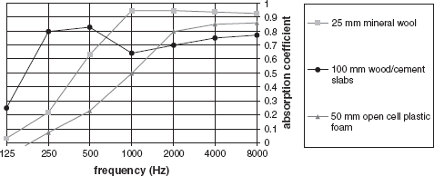
Figure 4.25:

Porous absorber fixed directly to a solid wall.

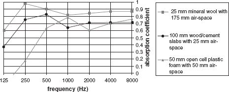
Figure 4.26:

Porous absorbers with air space behind. Note the increased low frequency absorption compared with Figure 4.25.

Before leaving the subject of porous absorbers let us consider the anechoic chamber construction shown in Figure 4.2. It can be seen that the porous/fibrous glass-fibre wool which is used as the absorbent material is in the form of wedges. In Table 4.1 we saw that the effect of thickness and density changes are such that more dense material was less absorbent weight for weight. This is partially because it presents more of a barrier to the arriving sound wave, which can enter into the pores of the less dense material more easily. So, because the surface necessarily presents a change in acoustic impedance from that of the air in the room, some proportion of the acoustic energy will be reflected back. The effect is somewhat like a lot of people all trying to pass through a few doors very quickly, but where they must keep walking at the same speed even if they cannot immediately enter a door. The only way is back! The wedges in the anechoic chamber present less of an abrupt obstacle to the encroaching acoustic wave, and so allow it to enter more gradually into the absorbent material. It also presents a greater surface area of material on each wall than could be provided by a plane surface of the same material. In fact, yet another function of the wedges is that they tend to produce the same amount of absorption independent of the angle of incidence of a sound wave, which in measuring chambers is another important point to be considered, even if it is not too relevant in studio situations.

4.5.5 Resonant Absorbers

In this category we have panel absorbers and Helmholtz absorbers. Figure 4.27 shows the construction of two typical panel absorbers, and Figure 4.28 shows a Helmholtz resonator in the form of a slotted concrete block. Unlike the fibrous/porous absorbers, which act on the velocity component of an acoustic wave, the resonant absorbers act on the pressure component of the wave (see Figures 4.9 and 4.10), so they are most effective when they are placed close to the hard boundaries of a room, where the pressure component of the resonant modes is at a maximum. When the panels are made of wood or plasterboard, for example, it is the internal frictional losses within the cellular or particulate make-up of the materials which converts the acoustic energy into heat, during the panel vibration. In the Helmholtz type of absorber, the frictional losses are due to the high particle velocities that occur in the openings at resonance.

The principle difference in effect between the fibrous/porous absorbers and the resonant absorbers is that the former generally tend to absorb better as the frequency increases, whereas the latter tend to function more effectively at lower frequencies. Figure 4.29 shows the typical sort of absorption curve to be expected from panel absorbers, and comparison with Figures 4.25 and 4.26 should prove interesting. For further comparisons, Figure 4.30 shows typical absorption curves for Helmholtz absorbers.

The frequency of peak absorption of a panel absorber is a function of the vibrating mass of the panel and the depth of the air space behind it. These are mass–spring systems, where the panel is the mass and the air cavity provides the spring. The stiffness of the spring is inversely proportional to the depth of the cavity, so, as the cavity increases in depth, the spring becomes less stiff and the resonant frequency drops. Increasing the mass of the panel also reduces the resonant frequency. All resonant absorbers are mass–spring systems, so in the case of the Helmholtz absorber, the air cavity again provides the spring, but this time the air slug in the neck of the resonator (the slot in the block in the case of Figure 4.28) provides the mass.

A variation on the Helmholtz absorber is the perforated sheet. Although the holes may seem to occupy only a very small proportion of the surface area, they act over a much greater area because of diffraction effects (see Section 4.8) which funnel the sound energy into each mouth from a much larger area. If the resonator mouths are less than a half-wavelength apart, they enhance each other’s radiation resistance and are then capable of absorbing a considerable range of frequencies around resonance.

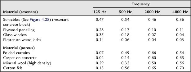
For comparison purposes, Table 4.2 shows the absorption coefficient at various frequencies for a selection of materials. The figures should not be taken as gospel truth, however, because differences inherent in the materials themselves, and in the way that they are applied, can have a great effect on their in-situ absorption. Nevertheless, the tendency can clearly be seen from the table that the porous/fibrous absorbers decrease in effect as the frequency lowers, whereas the resonant absorbers tend to increase in effectiveness as the frequency lowers.

4.5.6 Membrane Absorbers

These consist of a flexible, impervious sheet in place of the panel material shown in Figure 4.27. If the sheet is sufficiently ‘lossy’, and has a low bending stiffness, very significant amounts of acoustic energy can be turned into heat within the material of the sheet membrane. The air behind provides a damping spring. The membranes are typically plasticised bituminous material or mineral loaded flexible plastics. Polymer materials of high internal loss are also used. The early work on these absorbers was done by the BBC using bituminous roofing felt as the membrane. The trials were dogged by the tendency of the characteristics of the materials to change with temperature and time, and they were also inconsistent from batch to batch, even from the same manufacturer.

Specially produced materials are now in widespread use around the world, and many specialist acoustic material manufacturers have their own proprietary types. Dependent on use, such ‘deadsheets’, as they are commonly known, range in weight from around 3 to 15 kg/m². The lower weights are used more for acoustic control, whilst the higher weights are more effective for sound isolation. These materials will be considered further in later chapters. What these deadsheets have in common is that they are all very highly damped.

4.6 Q and Damping

Figure 4.31 shows the typical resonance peak of a standing wave in a highly reflective room. The high Q (quality factor) resonance exhibits a high concentration of energy around the resonant frequency, but very little activity only a few hertz away on either side of it. If any resonant absorber exhibits such a high Q resonance it will be characterised by a tendency to audibly ‘ring on’ after the acoustic drive signal has ceased. For this reason, acoustic absorber systems are usually heavily damped. The dashed line in Figure 4.31 shows the effect of damping the resonance. The peak of resonant activity is greatly reduced, but the width of the frequency range over which it resonates is considerably broadened. The tendency for the resonance to continue to ‘ring on’ after the drive signal has ceased is very much reduced. Damping, therefore, tends to be generally beneficial in terms of the desirable properties of acoustic absorbers. They absorb a wider range of frequencies more evenly, and they have fewer tendencies to re-radiate their resonant energy back into the room. However, lowering the Q does reduce the peak absorption, so for any given frequency more area must be used.

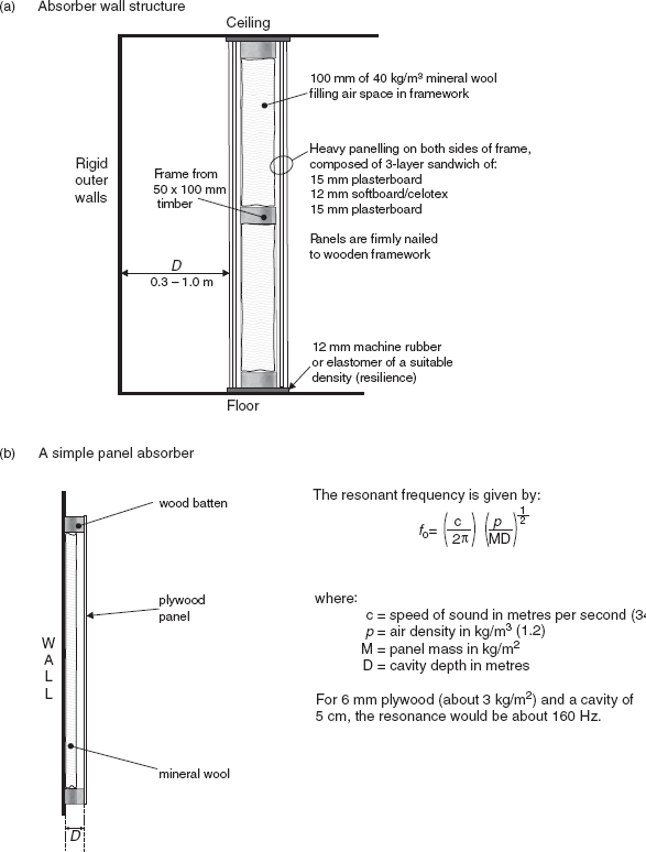
Figure 4.27:

(a, b) Panel absorbers: (a) Absorber wall structure. Panel absorber construction for providing absorption at low frequencies. This form of partitioning, often referred to as ‘Camden partitioning’, can be used to construct a complete self-standing room shell. The resonant frequency of such a structure would typically be about 20 Hz, but depends on the distance ‘D’, as well as the mass/rigidity/damping characteristics of the outer wall. (b) A simple panel absorber. The resonant frequency is given by:

where:

c = speed of sound in m/s (340)

ρ = air density in kg/m³ (1.2)

M = panel mass in kg/m²

D = cavity depth in m.

For 6 mm plywood (about 3 kg/m²) and a cavity depth of 5 cm, the resonance would be about 160 Hz.

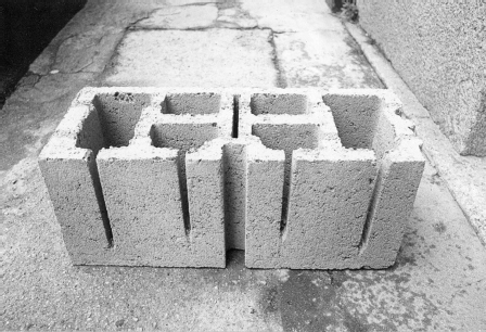
Figure 4.28:

Helmholtz resonator block.

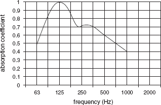
Figure 4.29:

Typical absorption characteristic to be expected from the panel absorber shown in Figure 4.27(b).

Damping refers to any mechanism which causes an oscillating system to lose energy. The damping of an acoustic wave can result from the frictional losses associated with the propagation of sound through porous material, the radiation of sound power, or by the internal frictional losses within any material or structure. From this it should be apparent that the damping losses within the materials reduce the Q of resonances within the materials themselves, and the absorption thus produced can, in turn, reduce the Q of the resonances within any room in which they are placed.

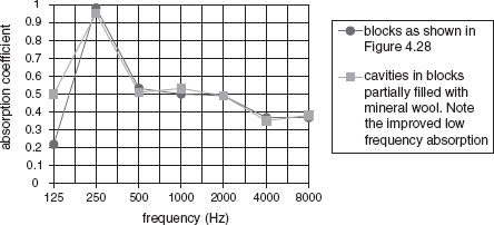
Figure 4.30:

Absorption characteristics of a Helmholtz resonator block.

Table 4.2: Absorption coefficients

4.7 Diffusion

The use of acoustic diffusers has been growing steadily since the 1980s. Convex and generally curved surfaces have been used since the design of early concert halls to re-radiate the incident sound over a wide area, and to break up the specular (i.e. behaving like light) reflexions which could tend to concentrate energy in specific areas (see Figure 4.32(a)). Again like absorbers, diffusive surfaces are linked in their size to the frequencies over which they are intended to have an effect. A low frequency diffuser of traditional design would need to be about a quarter of a wavelength deep in order to diffuse effectively.

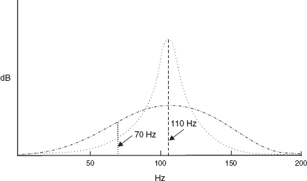
Figure 4.31:

The effect of damping on ‘Q’. The dotted line represents a high Q resonance, which will be strongly excited by a stimulus at 110 Hz but will respond only weakly to a stimulus at 70 Hz. The dashed line shows the effect of damping in lowering the Q. In this case, excitation at either 70 Hz or 110 Hz will produce an almost equal degree of resonance. Both the dashed and the dotted lines represent resonances with a 110 Hz centre frequency, and both contain a similar amount of total energy. It can thus be seen that the low Q resonance responds to a broader range of frequencies than the high Q resonance, but the low Q resonance can never achieve the same peak amplitude as the less damped high Q resonance if similarly excited.

Schroeder² and D’Antonio³ proposed designs for smaller diffusers using sequences of wells of different depths which are formally defined by mathematical sequences. To be effective, they still need to have an adequate depth, but the size is generally more manageable than the 1 m that a conventional convex diffuser would need in order to be effective in the 80–100 Hz region. Figure 4.32(b) shows the effect of a traditional tube/cylinder type diffuser, and Figure 4.32(c) shows the plan view of the well structure of a Schroeder-type diffuser.

In both cases, the incident wave is scattered in a wide range of directions other than the specular direction, where, like light, the angle of incidence equals the angle of reflexion, as shown in Figure 4.32(a). Diffusion is a form of scattering, but, where scattering tends to be more random in its effect and is often dependent upon the angle of incidence of the sound upon an irregular surface, effective diffusion aims to scatter the sound over a broader area, and a broader range of frequencies in a more spacially uniform manner. It is also less dependent upon the angle of incidence. In other words they are intended to scatter the energy equally in all directions. Angus⁴ has shown, however, that in some cases the mathematically based diffusers can create certain ‘hot spots’, or energy concentrations, that are even more concentrated than would be the case from a plane reflective surface. Nonetheless, this does not detract from the usefulness of such diffusers in many aspects of studio and auditorium acoustics.

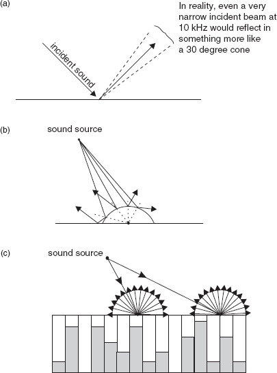
Figure 4.32:

(a) Specular reflexion. The concept of a specular reflexion is that it behaves like the reflexion of a beam of light. In fact this does not happen, because even a narrow beam of 10 kHz will still tend to reflect in a cone of about 30°. Nevertheless, the concept is useful; (b) Reflexion from curved surfaces. Although sound does not travel in narrow rays, the ray concept is useful to describe the diffusive effect of a semi-cylindrical surface. When the wavelength of the sound is longer than the diameter of the curved surface, the diffusive effect begins to reduce. For wavelengths much larger than the diameter of the curved surface, the effect is substantially the same as it would be if the surface were flat; (c) Reflexion from mathematically based diffusers. The concept of the Schroeder/reflective-phase-grating type of diffuser is for sounds of any angle of incidence to be reflected in all directions (two-dimensionally). The depth and distribution of the pits (wells) is determined mathematically, and is usually based on quadratic residues or prime number sequences. The maximum well depth determines the lowest frequency of good diffusion.

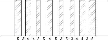
Figure 4.33:

Typical arrangement of wood strips and absorbent openings. The widths of the strips and openings are based on a numerical sequence that provides a more or less equal area of absorbent and reflective surfaces, but without any simple regularity, which could lead to problems at certain frequencies having properties coinciding with the regularity. The numbers in the diagram represent the relative dimensions of the adjacent strips and openings.

Another form of diffuse surface is the ‘amplitude reflexion grating’, an example of which is shown in Figure 4.33. In fact, any juxtaposition of absorbent and reflective surfaces will cause sound to scatter due to the steering of the wavefront as a result of phase changes at the boundary. There are also mathematical procedures for the optimum relative positioning of absorbent materials to promote diffusion,⁵ such as binary and prime number sequences. Amplitude reflexion gratings tend to diffuse not so well as the physically deeper diffusers, but they take up little depth, and the depth does not limit their low frequency performance. A flat, binary amplitude grating is shown in Figure 4.34.

4.8 Diffraction

Diffraction provides another form of acoustic energy scattering by the redirection of the incident energy. It is most commonly encountered at the discontinuities at the edges of partitions and screens, and is evident in control rooms at the edges of mixing consoles and rack furniture. Diffraction also occurs at the boundaries where absorbent and reflective surfaces meet. It is particularly problematical at the sharp edges of small loudspeaker boxes, where the edges can act like independent sound sources. This will be discussed later in Chapter 11. The fact that we are able to hold conversations over high, massive walls is totally thanks to the phenomenon of diffraction. However, the diffraction around complex objects can be hideously difficult to predict. Some of the earliest work on diffraction was done by the French physicist Augustin Fresnel, who invented the lighthouse lens, which is an example of light diffraction. Figure 4.35 shows some examples of diffraction, which clearly demonstrate its frequency dependent nature.

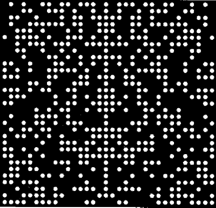
Figure 4.34:

Flat, binary amplitude grating.

Diffraction occurs due to the interaction between adjacent air molecules, because the compressions and rarefactions in a sound wave cannot simply shear at the boundary of an object without exciting the air nearby. If ever a picture told a thousand words, then it is exemplified by the photograph in Figure 4.36. It is also due to diffraction processes that a noise entering a room via a hole can be heard in most parts of the room, even if the room is very non-reflective.

4.9 Refraction

Acoustic refraction exists in fluids as a result of the spacial non-uniformity of the speed of sound. In air, if there is a non-uniformity of temperature in a given volume, the sound will travel at a greater speed in the warmer air, and so the wavefront will bend. It is mentioned here only to clarify the fact that it does not really enter into events in recording studios. It can be apparent at outdoor concerts when the temperature of the air changes with height, and it explains why some sounds can be heard a very great distance away from their source, yet at intermediate distances there is no perception of the sound whatsoever. In recording studios, even if temperature gradients do exist, the distances involved are much too small for refractive effects to be significant.

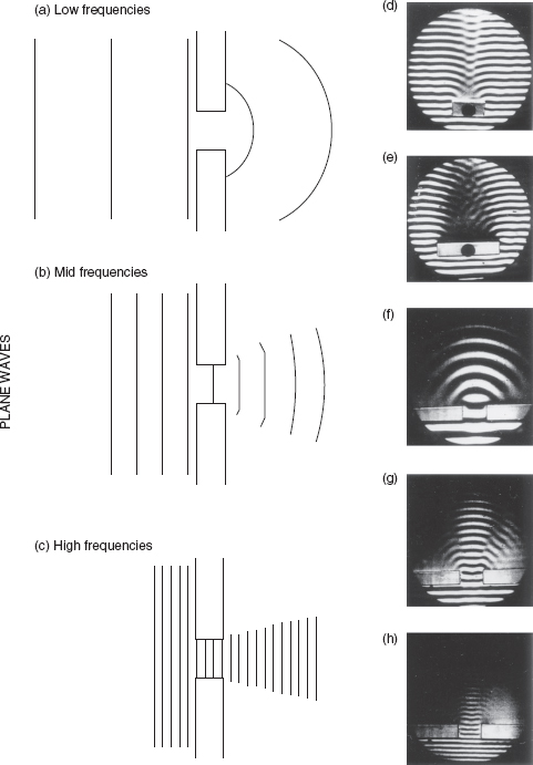
Figure 4.35:

(a–c) Frequency-dependent diffraction through a slot. Alternative presentation, in photographic form, shown in (f), (g) and (h). (d–h) Diffraction of a plane wave by: (d) narrow obstacle; (e) wide obstacle. Diffraction of a plane wave by an aperture in a screen: (f) at low frequency; (g) medium frequency; (h) high frequency. The photographs (d) to (h) were taken from Foundations of Engineering Acoustics, by Frank Fahy; Academic Press (2001) (original source unknown).

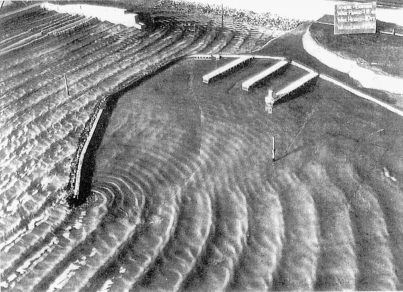
Figure 4.36:

Diffraction of water waves by a breakwater. Hydraulics Research Station, Wallingford, UK. Reproduced with permission from HMSO.

4.10 Review

Well, one chapter can hardly do justice to the subjects of room acoustics and their means of control, but it has been necessary to deal in a general way with them in order to provide a basis for the discussions which will follow. For more experienced readers, this chapter may have contributed little to their prior knowledge, but even so, a periodic recapitulation of the general concepts does no harm. Unfortunately, though, for a great number of people who are deeply involved in the professional recording industry, such information is not always very readily at hand, so without this discussion of some of the basic principles the remainder of the book would not be so accessible.

In fact, neither the performance of any musical instrument nor any loudspeaker can be realistically defined without a considerable knowledge of the acoustics of the rooms in which they are likely to be used. So, despite the frustrations inherent in the subject of room acoustics, we need to at least grasp the basics in some detail or our knowledge of recording studio design and performance will not be satisfactory. Those wishing greater in-depth knowledge of some of the relevant details are recommended to look at the References and the Bibliography at the end of the chapter.

4.11 Summary

A reflective isolation shell initially worsens the problems of internal acoustic control. A sound control room, well isolated, tends to start from a worse set of acoustics than exists in a normal domestic room.

Walls which are acoustically reflective create sonic images which are akin to the visible images of loudspeakers in a room with mirrors covering all surfaces. The reflexions behave as if they are coming from the distant loudspeakers which would be visible in the mirrors.

Flush mounted loudspeakers create less low frequency confusion in the room than do free-standing loudspeakers.

Sine waves give rise to axial, resonant standing wave patterns in a room with reflective walls when an integral number of half-wavelengths will fit exactly between two acoustically parallel surfaces.

The energy in an acoustic wave is continually changing between kinetic and potential as the velocity and pressure components, respectively, reach their maxima.

Modes are the pathways which a sound wave can take when travelling around a room. There are driven (forced) modes and resonant modes. It is the resonant modes which give rise to the standing/stationary wave patterns.

The lowest frequency of any mode in a room is that of the axial mode where one complete half-wavelength fits exactly between the two walls separated by the longest dimension of the room.

The resonant modal energy increases the loudness of a sound in a room, but unless the modes are closely spaced, they will favour some frequencies more than others, leading to an uneven frequency response.

Modal patterns depend on the shape of a room, and not its size. The size will determine the frequency range across which the pattern is distributed.

Flutter echoes result when a transient sound is produced between parallel reflective surfaces which are separated by more than about 8 m. With the surfaces separated by less distance, the result is a metallic ringing sound.

When the reflexion pattern becomes dense and spacially diffuse, reverberation is created. The reverberation time of a room is that which it takes for the reverberant field to decay by 60 dB after the sound source has been stopped.

As room size increases, the reverberation time increases proportionally if the average absorption remains constant.

Absorption is the most important factor in the control of room acoustics. The most common absorbers are porous absorbers, panel absorbers, membrane absorbers and Helmholtz absorbers.

Porous absorbers act on the particle velocity, by frictional and viscous losses. They are most effective away from wall surfaces and at higher frequencies.

Panel, membrane and Helmholtz absorbers are more effective at the boundaries of a room, and at low frequencies, because they react to the pressure component of an acoustic wave.

In air, due to the fact that it is a poor conductor of heat, the heat of compression and the cold of rarefaction both act to augment the speed of sound. If these heat changes can be reduced, such as by placing fibrous material in the air volume, then the speed of sound will be reduced. This can effectively enlarge a room (or a loudspeaker cabinet by up to 15%), due to the change from adiabatic to isothermal propagation.

The absorption coefficient of a material represents the proportion of a sound wave that is not reflected. Hence an open window is an almost perfect absorber, but it is not a good isolator. Isolation and absorption should not be confused. High isolation means low transmission. Isolation is usually achieved by reflective containment of the sound waves.

The Q of a resonance can be reduced by damping. Damping refers to any mechanism which causes an oscillating system to lose energy.

Diffusion is the re-radiation of an incident sound wave over a wide area.

Diffraction occurs at discontinuities at the edges of objects, and tends to bend the wavefront around the object. Edges which give rise to diffraction behave as separate sound sources.

Refraction is the process of the change in direction of a wavefront due to the spacial non-uniformity of the speed of sound. It is not usually encountered in recording studios, but may be apparent at outdoor music events when the air temperature changes with height.

References

1  Wright, J. R., ‘Increasing the Acoustic Compliance of Loudspeaker Cabinets’, Proceedings of the Institute of Acoustics [Reproduced Sound 17 Conference], Vol. 23, Part 8, pp. 23–8 (2001)

2  Scroeder, M. R., ‘Diffuse Sound Reflection by Maximum Length Sequences’, Journal of the Acoustical Society of America, Vol. 57, No. 1, pp. 149–50 (January 1975)

3  D’Antonio, P. and Konnert, J. H., ‘The Reflection Phase Grating Diffusor: Design, Theory and Application’, Journal of the Audio Engineering Society, Vol. 32, No. 4, pp. 228–38, (April 1984)

4  Angus, James A. S., ‘The Effects of Specular Versus Diffuse Reflections on the Frequency Response at the Listener’, Journal of the Audio Engineering Society, Vol. 49, No. 3, pp. 125–33, (March 2001)

5  Angus, J. A. S., ‘Sound Diffusers Using Absorption Gratings’, presented to the 98th Convention of the Audio Engineering Society, Paris, France, Preprint No. 3953 (February 1995)

Bibliography

Angus, James A. S. and McManmon, Claire I., ‘Orthogonal Sequence Modulated Phase Reflection Gratings for Wide-Band Diffusion’, Journal of the Audio Engineering Society, Vol. 46, No. 12, pp. 1109–18 (December 1998)

Borwick, John, Loudspeaker and Headphone Handbook, 3rd Edn, Focal Press, Oxford, UK (2001)

D’Antonio, P. and Cox, T., ‘Two Decades of Sound Diffusor Design and Development, Part 1: Application and Design’, Journal of the Audio Engineering Society, Vol. 46, No. 11, pp. 955–76 (November 1998)

D’Antonio, P. and Cox, T., ‘Two Decades of Sound Diffusor Design and Development, Part 2: Prediction, Measurement and Characterization’, Journal of the Audio Engineering Society, Vol. 46, No. 12, pp. 1075–91 (December 1998)

Davis, Don and Davis, Carolyne, Sound System Engineering, 2nd Edn, Focal Press, Oxford, UK, Boston, USA (1997)

Fahy, Frank, Foundation of Engineering Acoustics, Academic Press, London and San Diego (2001)

Howard, David M. and Angus, Jamie A. S., Acoustics and Psycoacoustics, 4th Edn, Focal Press, Oxford, UK (2009)

Parkin, P. H., Humphreys, H. R. and Cowell, J. R., Acoustics, Noise and Buildings, 4th Edn, Faber and Faber, London, UK (1979)