Chapter 2

Sound, Decibels and Hearing

2.1 Perception of Sound

That our perception of sound via our hearing systems is logarithmic becomes an obvious necessity when one considers that the difference in sound power between the smallest perceivable sound in a quiet room and a loud rock band in a concert is about 10¹² – one to one-million-million times. A rocket launch at close distance can increase that by a further one million times. The ear actually responds to the sound pressure though, which is related to the square root of the sound power, so the pressure difference between the quietest sound and a loud rock band is 10⁶ – one to one-million.

When a pure tone of mid frequency is increased in power by ten times, the tone will subjectively approximately double in loudness. This ten times power increase is represented by a unit called a bel. One tenth of that power increase is represented by a decibel (dB) and it just so happens that onedecibel represents the smallest mean detectable change in level that can be heard on a pure tone at mid frequencies. Ten decibels (one bel) represents a doubling or halving of loudness. However, the terms ‘pure tone’ and ‘mid frequencies’ are all-important here. Figure 2.1 shows two representations of equal loudness contours for human hearing. Each higher line represents a doubling of subjective loudness. It can be seen from the plots that at the frequency extremes the lines converge showing that, especially at low frequencies, smaller changes than 10 dB can be perceived to double or halve the loudness. This is an important fact that will enter the discussions many times during the course of this book.

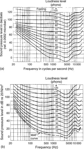
Figure 2.1 (a, b) Equal loudness contours. (a) The classic Fletcher and Munson contours of equal loudness for pure tones, clearly showing higher levels being required at high and low frequencies for equal loudness as the SPL falls. In other words, at 110 dB SPL, 100Hz, 1 kHz and 10 kHz would all be perceived as roughly equal in loudness. At 60 dB SPL, however, the 60 phon contour shows that 10 kHz and 100Hz would require a 10 dB boost in order to be perceived as equally loud to the 1 kHz tone. (b) The Robinson–Dadson equal loudness contours. These plots were intended to supersede the Fletcher–Munson contours, but, as can be seen, the differences are too small to change the general concept. Indeed other sets of contours have subsequently been published as further updates, but for general acoustical purposes, as opposed to critical uses in digital data compression and noise shaping, the contours of (a) and (b) both suffice. The MAF (minimum audible field) curve replaces the ‘0 phons’ curve of the older, Fletcher–Munson contours. The MAF curve is not absolute, but is statistically derived from many tests. The absolute threshold of hearing varies not only from person to person, but with other factors such as whether listening monaurally or binaurally, whether in free-field conditions or in a reverberant space, and the relative direction of the source from the listener. It is therefore difficult to fix an absolutely defined 0 dB curve

It is the concept of the doubling of loudness for every 10 dB increase in sound pressure level that fits so well with our logarithmic hearing. A street,  with light traffic in a small town will tend to produce a sound pressure level (SPL) of around 60 dBA, whereas a loud rock band may produce around 120 dBA (dB and dBA will be discussed later in the chapter). The sound pressure difference between 60 and 120 dBA is one thousand times, but it is self-evident that a loud rock band is not one thousand times louder than light traffic. If we use the 10 dB concept then 70 dBA will be twice as loud as 60 dBA, 80 dBA four times as loud (2 × 2), 90 dBA eight times (2 × 2 × 2), 100 dBA 16 times (2 × 2 × 2 × 2), 110 dBA 32 times (2 × 2 × 2 × 2 × 2), and 120 dBA 64 times as loud (2 × 2 × 2 × 2 × 2 × 2). The concept of a loud rock band being 64 times as loud as light traffic is more intuitively reasonable, and in fact it is a good approximation.

The concept of 1 dB being the smallest perceivable level change only holds true for pure tones. For complex signals in mid frequency bands it has been shown that much smaller level changes can be noticeable. Indeed, Dr Roger Lagadec, the former head of digital development at Studer International, in Switzerland, detected in the early 1980s audible colouration caused by amplitude response ripples in a digital filter at levels only just above ±0.001 dB. However, whether he was detecting the level changes, per se, or an artefact of the periodicity of the ripples, may still be open to question.

Perhaps it is therefore important to note at this early stage of the chapter that many so-called facts of hearing are often wrongly applied. Tests done on pure tones or speech frequently do not represent what occurs with musical sounds. Traditionally it has been the medical and communications industries that have funded much of the research into hearing. The fact that it is a different part of the brain which deals with musical perception to that which deals with speech and pure tones is often not realised. One should be very careful when attempting to apply known ‘facts’ about hearing to the subject of musical perception. They can often be very misleading.

2.2 Sound Itself

Sound is the human perception of vibrations in the region between 20Hz and 20kHz. ‘Hz’ is the abbreviation for hertz, the internationally accepted unit denoting cycles per second, or whole vibrations per second. The abbreviation ‘cps’ for cycles per second is still to be found in some older publications. (In some very old French texts, half-vibrations [zero-crossings] per second were used, with a consequent doubling of the frequency figure.¹) Figure 2.2 shows a graphic representation of a cycle of a sine wave. It can be seen that the pressure cyclically moves from compression to rarefaction and back to compression. The number of times which each whole cycle occurs in a second is known as the frequency. Hence, a frequency of 200Hz denotes that 200 cycles occur in any given second.

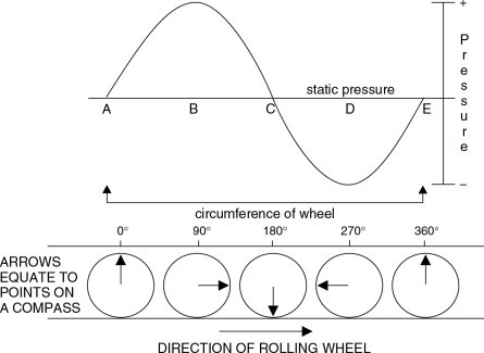
Figure 2.2 Sine wave; amplitude and phase. If the circumference of the wheel is equal to the period of the sine wave (A to E), then as the wheel rolls, a line drawn radially on the wheel will indicate the phase angle of the associated sine wave. This is why phase is sometimes denoted in radians – one radian being the phase angle passed through as the wheel advances by its own radial length on its circumference. Therefore, 360° = 2 π radians (i.e. circumference = 2 π × radius). 1 radian = 360°/2π = 57.3° approximately

The compression and rarefaction half cycles represent the alternating progression of the pressure from static pressure to its peak pressure, the return through static pressure and on to peak rarefaction, and finally back to static pressure. The whole cycle of a sine wave can be shown by an arrow placed on the perimeter of a rolling wheel whose circumference is equal to one wavelength. One complete revolution of the wheel could show one  whole cycle of a sine wave, hence any point on the sine wave can be related to its positive or negative pressure in terms of the degrees of rotation of the wheel which would be necessary to reach that point. One cycle can therefore be described as having a 360° phase rotation. The direction of the arrow at any given instant would show the phase angle, and the displacement of the arrowhead to the right or to the left of the central axle of the wheel would relate to the positive or negative pressures, respectively. The pressure variation as a function of time is proportional to the sine of the angle of the rotation of the wheel, producing a sinusoidal pressure variation, or sine wave.

Another way of describing 360° of rotation is 2π (pi) radians, a radian being the length on the circumference of the wheel which is equal to its radius. In some cases, this concept is more convenient than the use of degrees. The concept of a sine wave having this phase component leads to another definition of frequency: the frequency can be described as the rate of change of phase with time.

An acoustic sine wave thus has three components, its pressure amplitude, its phase, and time. They are mathematically interrelated by the Fourier transform. Fourier discovered that all sounds can be represented by sine waves in different relationships of frequency, amplitude and phase, a remarkable feat for a person born in the 18th century.

The speed of sound in air is constant with frequency, and is dependent only on the square root of the absolute temperature. At 20 °C it is around 344 m per second, sometimes also written 344 m/s or 344 m s⁻¹. The speed of sound in air is perhaps the most important aspect of room acoustics, because it dominates so many aspects of acoustic design. It dictates that each individual frequency will have its own particular wavelength. The wavelength is the distance travelled by a sound at any given frequency as it completes a full cycle of compression and rarefaction. It can be calculated by the simple formula:

(2.1)

where

λ = wavelength in metres

f = frequency

c = speed of sound in air

(344 metres per second at 20 °C)

For example, the wavelength of a frequency of 688Hz is:

The wavelength of 100Hz is:

To give an idea of the wavelength at the extremes of the audio frequency band, let us calculate the wavelengths for 20Hz and 20 kHz:

or 1.72 cm

Note the enormous difference in the wavelengths in the typical audio frequency range, from 17.2 metres down to 1.72 centimetres; a ratio of 1000:1.

There is also another unit used to describe a single frequency acoustic wave, which is its wave number. The wave number describes, in radians per metre, the cyclic nature of a sound in any given medium. It is thus the spacial equivalent of what frequency is in the time domain. It is rarely used by nonacademic acousticians, and is of little general use in the language of the studio world. Nevertheless, it exists in many text books, and so it is worth a mention, and helps once again to reinforce the concept of the relationship between sound and the world in which we live.

So what has all of this got to do with recording studios? A lot. An awful lot!

Sound is a wave motion in the air, and all wave motions, whether on the sea, through the earth (earthquakes), radio waves, light waves, or whatever else, follow many of the same universal physical laws. The spectrum of visible light covers about one octave, that is, the highest frequency involved is about double the lowest frequency. Sound, however, covers 20–40Hz, 40–80Hz, 80–160Hz, 160–320Hz, 320–640Hz, 640–1280Hz, 1280–2560Hz, 2560–5180Hz, 5180–10,360Hz, 10,360–20,720Hz . . . . 10 octaves, which one could even stretch to 12 octaves if one considers that the first ultrasonic and infrasonic octaves can contribute to a musical experience. That would mean a wavelength range from 34.4 metres down to 8.6 millimetres, and a frequency range not of 2 to 1, like light, but more in the order of 4000 to 1.

The ramifications of this difference will become more obvious as we progress in our discussions of sound isolation and acoustic control, but it does lead to much confusion in the minds of people who do not realise the facts. For example, as a general rule, effective sound absorption will take place when the depth of an absorbent material approaches one quarter of a wavelength. Many people know that 10 cm of mineral wool (Rockwool, Paroc, etc.), covering a wall, will absorb sound. Speech frequencies, around 1000Hz, with a wavelength of around 34 cm will be maximally absorbed, because the quarter wavelength would be 8.5 cm, so the 10 cm of absorbent would adequately exceed the quarter wavelength criterion. Indeed, all higher frequencies, with shorter wavelengths, would also be maximally absorbed. However, 100Hz, with a quarter wavelength of 85 cm (a wavelength of around 3.4 m), would tend to almost be totally unaffected by such a small depth of material. Nearly a one metre thickness would be needed to have the same effect at 100Hz as a 10 cm thickness at 1 kHz.

Figure 2.3 shows a medium sized anechoic chamber. The fibrous wedges are of one metre length, and they are spaced off from the walls in such a way that augments their low frequency absorption. The frequency having a four metre wavelength (one metre quarter wavelength) is 86Hz. With the augmentation effect of the spacing, the room is actually anechoic to around 70Hz. This means that all frequencies above 70Hz will be at least 99.9% absorbed by the boundaries of the room.

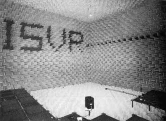
Figure 2.3 The ISVR anechoic chamber. The large anechoic chamber in the Institute of Sound and Vibration Research at Southampton University, UK, has a volume of 611 m³. The chamber is anechoic down to around 70Hz. Below this frequency, the wedges represent less than a quarter of a wavelength, and the absorption falls off with decreasing frequency. The floor grids are completely removable, but are strong enough to support the weight of motor vehicles

Contrast this to a typical voice studio with 10 cm of ‘egg-box’ type, foam wall coverings. For all practical purposes, this will be very absorbent above 800Hz, or so, and reasonably absorbent at 500Hz, or even a little below, but it will do almost nothing to control the fundamental frequencies of a bass guitar in the 40–80Hz range. This is why a little knowledge can be a dangerous thing. A person believing that thin foam wall panels are excellent absorbers, but not realising their frequency limitation, may use such treatments in rooms which are also used for the recording or reproduction of deep-toned instruments. The result is usually that the absorbent panels only serve to rob the instruments of their upper harmonics, and hence take all the life from the sound. The totally unnatural and woolly sound which results may be in many cases subjectively worse than the sound when heard in an untreated room. This type of misapplication is one reason why there are so many bad small studios in existence. The misunderstanding of many acoustic principles is disastrously widespread. (Section 5.11 deals with voice rooms in more detail).

So, is mineral wool absorbent? The answer depends on what frequency range we are considering, where it is placed, and what thickness is being used. The answer can vary from 100% to almost zero. Such is the nature of many acoustical questions.

2.3 The Decibel; Sound Power, Sound Pressure and Sound Intensity

The decibel is, these days, one of the most widely popularised technical terms. Strictly speaking, it expresses a power ratio, but it has many other applications. The dB SPL is a defined sound-pressure-level reference. Zero dB SPL is defined as a pressure of 20 micro pascals (one pascal being one newton per square metre) but that definition hardly affects daily life in recording studios. There are many text books which deal with the mathematics of decibels, but we will try to deal here with the more mundane aspects of its use. Zero (0) dB SPL is the generally accepted level of the quietest perceivable sound to the average, young human being.

Being a logarithmic unit, every 3 dB increase or decrease represents a doubling or halving of power. A 3 dB increase in power above 1 W would be 2 W, 3 dB more would yield 4 W, and a further 3 dB increase (9 dB above 1 W) would be 8 W. In fact, a 10 dB power increase rounds out at a 10 times increase in power, and this is a useful figure to remember.

Sound pressure doubles with every 6 dB increase, so one would need to quadruple the sound power from 1 W to 4 W (3 dB + 3 dB) to double the sound pressure from an acoustic source. Our hearing perception tends to correspond to changes in sound pressure level, and it was stated earlier that a roughly 10 dB increase or decrease was needed in order to double or halve loudness. What therefore becomes apparent is that if a 10dB increase causes a doubling of loudness, and that same 10 dB increase requires a ten times power increase (as explained in the last paragraph), then it is necessary to increase the power from a source by 10 times in order to double its loudness.

This is what gives rise to the enormous quantities of power amplifiers used in many public address (PA) systems for rock bands, because, in any given loudspeaker system, 100 W is only twice as loud as 10 W. One thousand watts is only twice as loud as 100 W, and 10 000 W is only twice as loud as 1000 W. Therefore, 10 000 W is only eight times louder than 10 W, and, in fact, only 16 times louder than 1 W. This is totally consistent with what was said at the beginning of the chapter, that a rock band producing 120 dB SPL was only about 64 times louder than light traffic, despite producing a thousand times more sound pressure. Yes, one million watts is only 64 times louder than 1 W – one million times the power produces one thousand times the pressure, which is 64 times louder at mid frequencies. The relationships need to be well understood.

Sound intensity is another measure of sound, but this time it deals with the flow of sound energy. It can also be scaled in decibels, but the units relate to watts per square metre. Sound waves in free space expand spherically. The formula for the surface area of a sphere is 4π × r² or 4πr². (Free air is often referred to as 4π space, relating to 4π steradians [solid radians].) The surface area of a sphere of 1 m radius (r) would thus be 4 × 3.142 (π = 3.142) × 1² or about 12.5 m². The surface area of a 2 m radius (r) sphere would therefore be 4π × 2² or 4 × 3.142 × 4, which is about 50m². So, every time the radius doubles, the surface area increases by four times.

Now, if the sound is made to distribute the same power over a four times greater area, then its intensity (in watts per square metre) must reduce by a factor of four. For the same total power in the system, each square metre will only have one quarter of the power over the surface of the 2 m radius sphere than it had on the surface of the 1 m radius sphere. One quarter of the power represents a reduction of 6 dB (3 dB for each halving), so the sound pressure at any point on the surface of the sphere will reduce by a half every time that one moves double the distance from the source of sound in free air. This is the basis of the often referred to ‘double-distance rule’ which states that as one doubles the distance from a sound source in free air, the sound pressure level will halve (i.e. fall by 6 dB).

Sound pressure level is represented by ‘SPL’. Sound power level is usually written ‘SWL’. The sound intensity is usually annotated ‘I’. From a point source in a free-field the intensity is the sound power divided by the area, or, conversely:

Sound power = sound intensity × area (or SWL = IA)

The sound intensity therefore falls with the sound pressure level as one moves away from a source in a free-field. In a lossless system, they would both reduce with distance, even though the total sound power remained constant, merely spreading themselves thinner as the surface area over which they were distributed increased.

2.3.1 The dBA and dBC Scales

Reference has already been made, in earlier sections, to dB SPL and dBA. Essentially, a sound level meter consists of a measuring microphone coupled to an amplifier which drives a meter calibrated in dB SPL, referenced to the standard 0 dB SPL. The overall response is flat. Such meters are used for making absolute reference measurements. However, as we saw from Figure 2.1, the response of the human hearing system is most definitely not flat. Especially at lower levels, the ear is markedly less sensitive to low and high frequencies than it is to mid frequencies. It can be seen from Figure 2.1 that 60 dB SPL at 3 kHz will be very audible, in fact it will be over 60 dB above the threshold of hearing at that frequency, yet a tone of 30Hz would be inaudible at 60 dB SPL; it would lie on the graph below the 0 phon curve of ‘just audible’.

Consequently, if a flat reading of 60 dB was taken on an SPL meter measuring a broad-band noise signal in a room, then 25 dB of isolation would be needed at 3 kHz if the neighbours were not to be subjected to more than 35 dBA. However, at 30Hz, nothing would need to be done, because the sound at that frequency would not even be audible in the room, let alone outside of it. Hence, providing 25 dB of isolation at 30Hz to reduce the outside level to less than 35 dB SPL unweighted (i.e. a flat frequency response) would simply be a waste of time, money, effort and space.

To try to make more sense from the noise measurements, an ‘A-weighting’ filter is provided in the amplifier circuits of most SPL meters, which can be switched in when needed. The ‘A’ filter is approximately the inverse of the 40 phon curve from the equal loudness contours of Figure 2.1, and is shown in Figure 2.4. The effect of the A-weighting is to render the measurement at any frequency (at relatively low SPLs), subjectively equal. That is to say, a measurement of 40 dBA at 40Hz would sound subjectively similar in level as a measurement of 40 dBA at 1 kHz, or 4 kHz, for example. This greatly helps with subjective noise analysis, but A-weighting should never be used for absolute response measurements such as the flatness of a loudspeaker. For such purposes, only unweighted measurements should be used.

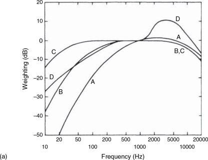
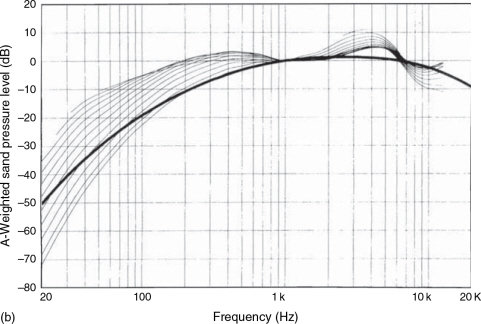
Figure 2.4 (a) A-, B-, C- and D-weighting curves for sound level meters. (b) Inverse equal loudness level contours for a diffuse field for the range from the hearing threshold to 120 phon (thin lines), and A-weighting (thick line). The above figure was taken from ‘On the Use of A-weighted Level for Prediction of Loudness Level’, by Henrik Müller and Morten Lydolf, of Aalborg University, Denmark. The paper was presented to the 8th International Meeting on Low Frequency Noise and Vibration, in Gothenburg, Sweden, in June 1997. The work is published in the Proceedings, by Multi-Science Publishing, UK

Also shown in Figure 2.4 is the ‘C-weighting’ curve. This roughly equates to the inverse of the 80 phon curve of Figure 2.1. C-weighting is more appropriate than A-weighting when assessing the subjectivity of higher level noises, but as it is the nuisance effect of noise that is usually of most concern, the C-weighting scale is less widely used. There is also a ‘B-weighting’ curve, but it is now largely considered to be redundant, especially as no current legislation makes use of it.

One must be very careful not to mix the measurements because there is no simple way of cross-referencing them. In the opening paragraphs of this chapter reference was made to a loud rock band producing 120 dBA. Strictly speaking, the use of the dBA scale in the region of 120 dB SPL is a nonsense, because the A curve does not even vaguely represent the inverse of the response of the ears at the 120 phon loudness level, shown in Figure 2.1, which is almost flat. The 120 phon level actually equates better to an unweighted response, but, as has just been mentioned, one cannot mix the use of the scales. It would have been more accurate to say that a very loud rock band at 120dBA would, in the mid frequency range, be 64 times louder than light traffic in the street of a small town. The low frequencies may in fact, sound very much louder.

This fact affects the thinking on sound isolation, which can also be rated in dBA. There are measurements known as Noise Criteria (NC) and Noise Ratings (NR) which are close to the dBA scale. They allow for reduced isolation as the frequency lowers, in order to be more realistic in most cases of sound isolation, although they are perhaps more suited to industrial noise control than to recording studio and general music use. Where very high levels of low frequencies are present, such as in recording studios, 60 dB of isolation at 40Hz may well be needed, along with 80 dB of isolation at 1 kHz, in order to render both frequencies below the nuisance threshold in adjacent buildings. An NR, NC or A-weighted specification for sound isolation would suggest that only 40 dB of isolation were necessary at 40Hz, not 60 dB, so it would underestimate by 20 dB the realistic isolation needed. Not many industrial processes produce the low frequency SPLs of a rock band.

If all of this sounds a little confusing, it is because it is. The non-flat frequency response of the ear and its non-uniform dynamic response (i.e. the frequency response changes with level) have blighted all attempts to develop a simple, easily understood system of subjective/objective noise level analysis. Although the A-weighting system is very flawed, it nevertheless has proved to be valuable beyond what could ever have been academically expected of it. However, all of these measurements require interpretation, and that is why noise control is a very important, independent branch of the acoustical sciences. Failing to understand all the implications of the A, C and unweighted scales has led to many expensive errors of studio construction, so if the situation is serious, it is better to call in the experts.

2.4 Human Hearing

The opening section of this chapter, although making many generalisations, hinted at a degree of variability in human perception. By contrast, the second section dealt with what is clearly a hard science; that of sound and its propagation. Acoustic waves behave according to some very set principles, and despite the interaction at times being fiendishly complex, acoustics is nevertheless a clearly definable science. Likewise in the third section, the treatment of the decibel is clearly mathematical, and it is only its application to human hearing and perception where it begins to get a little ragged. It is however the application that gets ragged, not the concept of the decibel itself. Eventually, though, we must understand a little more about the perception of sound by individual human beings, because they are the final arbiters of whatever value exists in the end result of all work in recording studios, and it is here where the somewhat worrying degree of variability enters the proceedings in earnest.

The world of sound recording studios is broad and deep. It straddles the divide between the hardest objective science and the most ephemeral art, so what the rest of this chapter will concentrate on is the degree of hearing variability which may lead many people to make their own judgements. These judgements relate both to the artistic and scientific aspects of the recording studios themselves, and the recordings which result from their use.

The human auditory system is truly remarkable. In addition to the characteristics described in earlier sections, it is equipped with protection systems which limit ear drum (tympanic membrane) movement below 100Hz. These are to prevent damage, yet still allow the brain to interpret, via the help of body vibration conduction, what is really there. The ear detects pressure half-cycles, which the brain re-constructs into full cycles, and can provide up to 15 dB of compression at high levels. By means of time, phase and amplitude differences between the arrivals of sound at the two ears, we can detect direction with great accuracy, in some cases to as little as a few degrees. Human pinnae (outer ears) have evolved with complex resonant cavities and reflectors to enhance this ability, and to augment the level-sensitivity of the system.

Our pinnae are actually as individual to each one of us as are our fingerprints, which is the first step in ensuring that our overall audio perception systems are also individual to each one of us. When we add all of this together, and consider the vagaries introduced by what was discussed in Section 2.3.1, we should be able to easily realise how the study of acoustics, and audio in general, can often be seen as a black art. Hearing perception is a world where everything seems to be on an individually sliding scale. Of course, that is also one reason why it can be so fascinating. However, until it is sufficiently understood, frustration can often greatly outweigh fascination.

Psychoacoustics is the branch of the science which deals with the human perception of sound, and it has made great leaps forward in the past 25 years, not least because of the huge amount of money pumped into research by the computer world in their search for ‘virtual’ everything. Psychoacoustics is an enormous subject, and the bibliography at the end of this chapter suggests further reading for those who may be interested in studying it in greater depth. Nevertheless, it may well be useful and informative to look at some concepts of our hearing, and its individuality with respect to each one of us, because it is via our own hearing that we each perceive and judge musical works. From the differences which we are about to explore, there can be little surprise if there are some disagreements about standards for recording studio design.

What follows was from an article in Studio Sound magazine, in April 2000.

2.4.1 Chacun a Son Oreille

In 1896, Lord Rayleigh wrote in his book, The Theory of Sound (Strutt, 1896, p. 1) ‘The sensation of a sound is a thing sui generis, not comparable with any of our other senses. . . . Directly or indirectly, all questions connected with this subject must come for decision to the ear, . . . and from it there can be no appeal’. Sir James Jeans concluded his book Science & Music (Cambridge University Press, 1937) with the sentence ‘Students of evolution in the animal world tell us that the ear was the last of the sense organs to arrive; it is beyond question the most intricate and the most wonderful’.

The displacement of the ear drum when listening to the quietest perceivable sounds is around one-hundredth of the diameter of a hydrogen molecule, and even a tone of 1 kHz at a level of 70 dB still displaces the ear drum by less than one-millionth of an inch (0.025 micrometres). Add to all these points the fact that our pinnae (outer ears) are individual to each one of us, and one has a recipe for great variability in human auditory perception as a whole, because the ability to perceive these minute differences is so great.

In fact, if the ear was only about 10 dB more sensitive than it is, we would hear a permanent hiss of random noise, due to detection of the Brownian motion of the air molecules. Some people can detect pitch changes of as little as 1/25th of a semitone (as reported by Seashore). Clearly there is much variability in all of this from individual to individual, and one test carried out on 16 professionals at the Royal Opera, Vienna, showed a 10:1 variability in pitch sensitivity from the most sensitive to the least sensitive. What is more, ears all produce their own non-linear distortions, both in the form of harmonic and inter-modulation distortions. I had one good friend who liked music when played quietly, but at around 85 dB SPL she would put her hands to her ears and beg for it to be turned down. It appeared that above a certain level, her auditory system clipped, and at that point all hell broke loose inside her head.

Of course, we still cannot enter each other’s brains, so the argument about whether we all perceive the colour blue in the same way cannot be answered. Similarly we cannot know that we perceive what other people hear when listening to similar sounds under similar circumstances. We are, however, now capable of taking very accurate in-ear measurements, and the suggestion from the findings is that what arrives at the eardrums of different people is clearly not the same, whereas what enters different people’s eyes to all intents and purposes is the same. Of course, some people may be colourblind, whilst others may be long-sighted, short-sighted, or may have one or a combination of numerous other sight anomalies. Nevertheless, what arrives at the eye, as the sensory organ of sight, is largely the same for all of us. However, if we take the tympanic membrane (the ear drum) as being the ‘front-end’ of our auditory system, no such commonality exists. Indeed, even if we extend our concept of the front-end to some arbitrary point at, or in front of, our pinnae, things would still not be the same from person to person because we all have different shapes and sizes of heads and hair styles. This inevitably means that the entrances to our ear canals are separated by different distances, and have different shapes and textures of objects between them. Given the additional diffraction and reflexion effects from our torsos, the answer to the question of whether we all ‘see the same blue’ in the auditory domain seems to be clearly ‘no’, because even what reaches our ear drums is individual to each of us, let alone how our brains’ perceive the sounds.

There is abundant evidence to suggest that many aspects of our hearing are common to almost all of us, and this implies that there is a certain amount of ‘hard-wiring’ in our brains which predisposes us towards perceiving certain sensations from certain stimuli. Nevertheless, this does not preclude the possibility that some aspects of our auditory perception may be inherited, and that there may be a degree of variability in these genetically influenced features. Aside from physical damage to our hearing system, there may also be cultural or environmental aspects of our lives which give rise to some of us developing different levels of acuteness in specific aspects of our hearing, or that some aspects may be learned from repeated exposure to certain stimuli.

It would really appear to be stretching our ideas of the evolutionary process beyond reason, though, to presume that the gene pairings which code our pinnae could somehow be linked to the gene pairings which code any variables in our auditory perception systems. Furthermore, it would seem totally unreasonable to expect that if any such links did exist, that they could function in such a way that one process could complement the other such that all our overall perceptions of sound were equal. In fact, back in the 1970s, experiments were carried out (which will be discussed in later paragraphs) which more or less conclusively prove that this could not be the case. Almost without doubt, we do not all hear sounds in the same way, and hence there will almost certainly always be a degree of subjectivity in the judgement and choice of studio monitoring systems. There will be an even greater degree of variability in our choice of domestic hi-fi loudspeakers, which tend to be used in much less acoustically controlled surroundings.

Much has been written about the use of dummy head recording techniques for binaural stereo, and it has also been frequently stated that most people tend to perceive the recordings as sounding more natural when they are made via mouldings of their own pinnae. In fact, many people seem to be of the opinion that we all hear the recordings at their best if our own pinnae mouldings are used, but this is not necessarily the case. It is true that the perception may be deemed more natural by reference to what we hear from day-to-day, but it is also true that some people naturally hear certain aspects of sound more clearly than others. In my first book,² I related a story about being called to a studio by its owner, to explain why hi-hats tended to travel in an arc when panned between the loudspeakers; seeming to come from a point somewhere above the control room window when centrally panned. The owner had just begun to use a rather reflexion-free control room, in which the recordings were rendered somewhat bare. On visiting the studio, all that I heard was a left-to-right, horizontal pan. We simply had different pinnae.

In a well-known AES paper, and in her Ph.D. thesis, the late Puddie Rodgers³,⁴ described in detail how early reflexions from mixing consoles, or other equipment, could cause response dips which mimicked those created by the internal reflexions from the folds and cavities of different pinnae when receiving cues from different directions. In other words, a very early reflexion from the surface of a mixing console could cause comb filtering of a loudspeaker response which could closely resemble the in-ear reflexions which may cause a listener to believe that the sound was coming from a direction other than that from which it was actually arriving. Median plane vertical perception is very variable from individual to individual, and in the case mentioned in the last paragraph, there was almost certainly some source of reflexion which gave the studio owner a sensation of the high frequencies arriving from a vertically higher source, whilst I was left with no such sensation. The differences were doubtless due to the different shapes of our pinnae, and the source of reflexions was probably the mixing console.

In the ‘letters’ page of the October 1994 Studio Sound magazine, recording engineer Tony Batchelor very courageously admitted that he believed that he had difficulty in perceiving what other people said stereo should be like. He went on to add, though, that at a demonstration of Ambisonics he received ‘a unique listening experience’. Clearly to Tony Batchelor, stereo imaging would not be at the top of his list of priorities for his home hi-fi system, yet he may be very sensitive to intermodulation distortions, or frequency imbalances, to a degree that would cause no concern to many other people.

Belendiuk and Butler⁵ concluded from their experiments with 45 subjects that ‘there exists a pattern of spectral cues for median sagittal plane positioned sounds common to all listeners’. In order to prove this hypothesis, they conducted an experiment in which sounds were emitted from different, numbered, loudspeakers, and the listeners were asked to say from which loudspeaker the sound was emanating. They then made binaural recordings via moulds of the actual outer ears of four listeners, and asked them to repeat the test, via headphones, of the recordings made using their own pinnae. The headphone results were very similar to the direct results, suggesting that the recordings were representative of ‘live’ listening. Not all the subjects were equally accurate in their correct choices, with some, in both their live and recorded tests, scoring better than others in terms of identifying the correct source position.

Very interestingly, when the tests were repeated with each subject listening via the pinnae recordings of the three other subjects in turn, the experimenters noted, ‘that some pinnae, in their role of transforming the spectra of the sound field, provide more adequate (positional) cues .. . than do others’. Some people, who scored low in both the live and recorded tests, using their own pinnae, could locate more accurately via other peoples’ pinnae. Conversely, via some pinnae, none of the subjects could locate very accurately. The above experiments were carried out in the vertical plane. Morimoto and Ando,⁶ on the other hand, found that, in the horizontal plane, subjects generally made fewer errors using their own head-related transfer functions (HRTFs), i.e. via recordings using simulations of their own pinnae and bodies. What all the relevant reports seem to have shown, over the years, is that different pinnae are differently perceived, and the whole HRTF is quite distinct from one person to another. All of these differences relate to the different perceptions of different sound fields.

Studio Monitoring Design (Newell, 1995)² also related the true story of two well-respected recording engineers who could not agree on the ‘correct’ amount of high frequencies from a monitor loudspeaker system which gave the most accurate reproduction when compared to a live cello. They disagreed by a full 3 dB at 6 kHz, but this disagreement was clearly not related to their own absolute high frequency sensitivities because they were comparing the sound of the monitors to a live source. The only apparent explanation to this is that because the live instrument and the loudspeakers produced different sound fields, the perception of the sound field was different for each listener. Clearly, all the high frequencies from the loudspeaker came from one very small source, the tweeter, whilst the high frequency distribution from the instrument was from many points – the strings and various parts of the body. The ‘highs’ from the cello radiated, therefore, from a distributed source having a much greater area than the tweeter. Of course, the microphone could add its own frequency tailoring and one-dimensionality, but there would seem to be no reason why the perception of this should differ from one listener to another.

So, given the previous discussion about pinnae transformations and the different HRTFs as they relate to sounds arriving from different directions, it does not seem too surprising that sound sources with spacially different origins may result in spectrally different perceptions for different people. Tony Batchelor’s statements about his not being able to appreciate stereo, yet readily perceiving Ambisonic presentations of spacial effects, would seem to be strongly related to aspects of the sound field. He and I would no doubt attach different degrees of importance to the horizontal effects of stereo if working on a joint production. Martin Young (the aforementioned studio owner) and I clearly had different vertical perception when panning a hi-hat; and the two well-known engineers could not agree on a natural high-frequency level in a live versus loudspeaker test.

The implications of all this would suggest that unless we can reproduce an accurate sound field, we will never have universal agreement on the question of ‘the most accurate’ monitoring systems. Add to this a good degree of personal preference for different concepts of what constitutes a good sound, and it would appear that some degree of monitoring and control room variability will be with us for the foreseeable future. Nevertheless, the last 20 years have seen some very great strides forward in the understanding of our auditory perception systems, and this has been a great spur to the advancement of loudspeaker and control room designs. Probably, though, we have still barely seen the tip of the iceberg, so it will be interesting to see what the future can reveal.

To close, let us look at some data that has been with us for 40 years, or more. The plots shown in Figures 2.5 and 2.6 were taken from work by Shaw.⁷ Figure 2.5 shows the average, in-ear-canal, 0° and 90° responses for ten people. Note how the ear canal receives a very different spectrum depending upon the direction of arrival of the sound. Figure 2.6 shows the ten individual sources from which Figure 2.5 was derived. The differences from person to person are significant, and the response from one direction cannot be inferred from the response from a different direction.

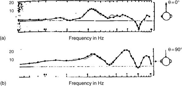
Figure 2.5 Shaw’s data showing the ratio (in dB) of the sound pressure at the ear canal entrance to the free field sound pressure. The curves are the average of ten responses. (a) shows the average response for a sound source at 0° azimuth and (b) shows the average response for a sound source at 90° azimuth

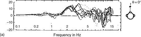
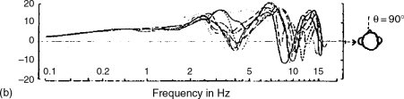
Figure 2.6 Shaw’s data showing the ratio (in dB) of the sound pressure at the ear canal entrance to the free field sound pressure. (a) shows the response for each of the ten subjects for a sound source of 0° azimuth. (b) shows the response for a sound source at 90° azimuth

Given these differences, and all of the aspects of frequency discrimination, distortion sensitivity, spectral response differences, directional response differences, psychological differences, environmental differences, cultural differences, and so forth, it would be almost absurd to expect that we all perceive the same balance of characteristics from any given sound. It is true that whatever we each individually hear is natural to each one of us, but when any reproduction system creates any imbalance in any of its characteristics, as compared to a natural event, the aforementioned human variables will inevitably dictate that any shortcomings in the reproduction system will elicit different opinions from different people vis-à-vis the accuracy of reproduction. As to the question of whether it is more important to reduce the harmonic distortion in a system by 0.02%, or the phase accuracy of 5° at 15 kHz, it could well be an entirely personal matter, and no amount of general discussion could reach any universal consensus. Indeed, Lord Rayleigh was right; the sensation of sound is a thing, sui generis (sui generis meaning ‘unique’).

2.5 Summary

Hearing has a logarithmic response to sound pressures because the range of perceivable sound pressures is over one-million to one. It is hard to imagine how we would hear such a range of pressure levels if hearing were based on a linear perception.

One decibel approximates to the smallest perceivable change in level for a single tone. At mid frequencies, 10 dB approximates to a doubling or halving of perceived loudness. Doubling the loudness requires ten times the power.

The speed of sound in air is constant with frequency, (but this is not so in most other substances). The speed of sound in any given material determines the wavelength for each frequency.

The spectrum of visible light covers about one octave, but the spectrum of audible sound covers more than 10 octaves. This leads to wavelengths differing by 1000 to 1 over the 20Hz to 20 kHz frequency range – 17.4 m to 1.74 cm.

How absorbers behave towards any given sound is dependent upon the relationship between size and wavelength.

The decibel is the most usual unit to be encountered in measurements of sound. Sound power doubles or halves with every 3dB change. Sound pressure doubles or halves with every 6 dB change. Our hearing system responds to changes in sound pressure.

Sound intensity is the flow of sound energy, and is measured in watts per m².

Sound decays by 6dB for each doubling of distance in free-field conditions, because the intensity is reduced by a factor of four on the surface of a sphere each time the radius is doubled.

The dBA scale is used to relate better between sound pressure measurements and perceived loudness at low levels.

The dBC scale is more appropriate for higher (around 80 dB) sound pressure levels.

For equipment response measurements, or any absolute measurements, only a flat (unweighted) response should be used.

Sound isolation need not be flat with frequency because our perception of the loudness of the different frequencies is not uniform.

Our pinnae are individual to each one of us, so to some extent we all perceive sounds somewhat differently.

Psychoacoustics is the branch of the science which deals with the human perception of sound.

The displacement of the ear drum by a sound of 0 dB SPL is less than one one-hundredth of the diameter of a hydrogen molecule.

Some people can detect pitch changes of as little as one 1/25th of a semitone. Due to the physical differences between our bodies, and especially our outer ears, the sounds arriving at our ear drums are individual to each one of us.

Some pinnae perform better than others in terms of directional localisation. The differences in perception between different people can give rise to different hierarchies of priorities in terms of what aspects of a sound and its reproduction are most important.

Perception of musical instrument, directly or via loudspeakers, can be modified by pinnae differences; so the loudspeaker that sounds most accurate to one person may not be the one that sounds most accurate to another person.

References

1  Tyndall, John, On Sound, 6th edn, Longmans, Green & Co., London, UK, p. 67 (1895)

2  Newell, Philip. Studio Monitoring Design, Focal Press, Oxford, UK, and Boston, USA (1995)

3  Rodgers, Carolyn Alexander, Ph.D. Thesis, Multidimensional Localization, Northwestern University, Evanston, IL, USA (1981)

4  Rodgers, Puddie C. A., ‘Pinna Transformations and Sound Reproduction’, Journal of the Audio Engineering Society, Vol. 29, No. 4, pp. 226–234 (April 1981)

5  Belendiuk, K. and Butler, R. A., ‘Directional Hearing Under Progressive Improvement of Binaural Cues’, Sensory Processes, 2, pp. 58–70 (1978)

6  Morimoto, M. and Ando, Y. ‘Simulation of Sound Localisation’, presented at the Symposium of Sound Localisation, Guelph, Canada (1979)

7  Shaw, E. A. G., ‘Ear Canal Pressure Generated by a Free-Field Sound’, Journal of the Acoustical Society of America, Vol. 39, No. 3, pp. 465–470 (1966)

Bibliography

Borwick, John, Loudspeaker and Headphone Handbook, 3rd Edn, Focal Press, Oxford, UK (2001)

Davis, Don, and Davis, Carolyne, Sound System Engineering, 2nd Edn, Focal Press, Boston, USA (1997)

Howard, David M. and Angus, James, Acoustics and Psychoacoustics, 2nd Edn, Focal Press, Oxford, UK (2001)

Strutt, John William, 3d Baron Rayleigh, The Theory of Sound, 2nd edn, Vol. 1, London (1896). Republished by Dover Publications, New York (1945) (still in print, 2007)