
Chapter 4: Slicing and Dicing Data with OLAP Cubes
4.2 OLAP Cube: Concepts and Definitions
4.3 Building a Cube with SAS OLAP Cube Studio
4.3.1 Creating a Cube Using the Cube Designer
4.3.2 Adding Calculated Items to the Cube
4.4 Using OLAP Cubes with SAS AMO
4.4.1 Essentials of OLAP Analyzer
4.4.2 Adding Measures and Moving Dimensions
4.4.3 Slicing and Dicing in the OLAP Analyzer
4.4.5 Creating Computed Measures
4.4.6 Conditional Highlighting
4.4.7 Bookmarking A Customized Cube View
4.1 Introduction
Analysts in the Finance department at Healthy Living Inc. feel empowered with SAS Add-In for Microsoft Office. They now run their own monthly reports using SAS stored processes. They analyze and research data instead of placing these tasks in the queue for the overscheduled SAS programmers in the IT department.
The analysts retrieve information at both summary and detail levels, but they find this process laborious and piecemeal. They want to traverse the information highway quickly, seamlessly navigating from summary to detail data.
A SAS OLAP cube enables analysts to slice and dice data to get to the details. This chapter builds a simple, yet effective, cube using SAS OLAP Cube Studio. It shows analysts how to use this cube in Excel with SAS Add-In for Microsoft Office.
4.2 OLAP Cube: Concepts and Definitions
The acronym “OLAP” stands for online analytical processing. The word “cube” conjures up its namesake geometrical shape. However, neither the acronym nor the word is helpful in understanding what an OLAP cube is.
It might be easier to understand what an OLAP cube is by comparing it with a familiar entity, the SAS data set. A SAS data set is usually a single file, arranged by columns and rows in a tabular format. In contrast, an OLAP cube is a series of files in a folder. Each file contains unique information about key metrics and is connected to the other files in a hierarchical and multidimensional manner. The nature of the connections between the various components of a cube enables you to slice and dice your way through the data.
It’s important to understand basic OLAP terminology and concepts. Consider the Encounter table, which contains key metrics such as paid and charged amounts. It has various slicer variables, including date of service, category, and diagnosis.
The sole purpose of a cube is to examine how key metrics vary by slicer variables. An analyst might want to examine paid amount by category, diagnosis, and date of service, or a combination thereof.
Slicer variables can be categorized into logical groupings or dimensions. Because Category and Diagnosis belong in a logical group, they can be placed in a dimension called Service Type, with Category appearing before Diagnosis. The sequential ordering of variables in a dimension is called a hierarchy.
A dimension can have more than one hierarchy. For example, consider the Time dimension and the following two hierarchies:
1. Year > Month > Day
2. Year > Quarter > Month > Day
A cube can include calculated elements, and it has the ability to perform calculations dynamically. An example of a computed item is the paid/charged amounts ratio.
SAS OLAP Cube Studio provides step-by-step directions for building and editing a cube through its wizard, the Cube Designer.
1. A dimension can be thought of as a container of variables. The variables are called levels. Their logical ordering is called a hierarchy. The value of a level is called a member. Consider this example. The Time dimension has the following levels: Year, Month, and Day. The ordering of levels, beginning with Year and ending with Day, is called a hierarchy. January is a member of the Month level.
2. The SAS developer can bypass SAS OLAP Cube Studio entirely. A cube can be created, edited, and maintained using the OLAP procedure.
4.3 Building a Cube with SAS OLAP Cube Studio
This section creates an effective cube using the Encounter table.
4.3.1 Creating a Cube Using the Cube Designer
1. From the File menu, select New → Cube. This begins the Cube Designer wizard, which provides step-by-step assistance with creating and editing cubes.
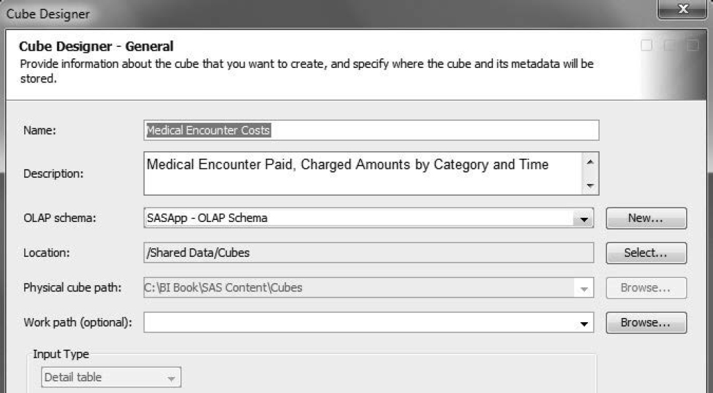
2. On the General page, enter the following information as shown in Figure 4.1:
a. Enter the name of the cube in Name.
b. Enter a short description of the cube in Description.
c. For OLAP schema, select an OLAP schema to hold a collection of like cubes. SASApp - OLAP Schema is selected by default.
d. For Location, specify that the cube is to be saved in the user-created Cubes folder.
e. For Physical cube path, specify the location where the cube is to be stored.
f. For Work path, specify the location where the cube stores its temporary files. If this value is left blank, SAS uses a default value.
g. For Input Type, select Detail table because Encounter contains non-summarized data.
Figure 4.1: Provide Information about a Cube
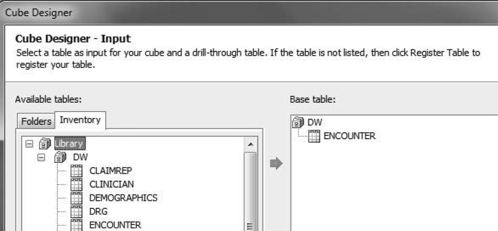
3. On the Input page, move Encounter to Base table.
Figure 4.2: Select Detail Table in a Cube
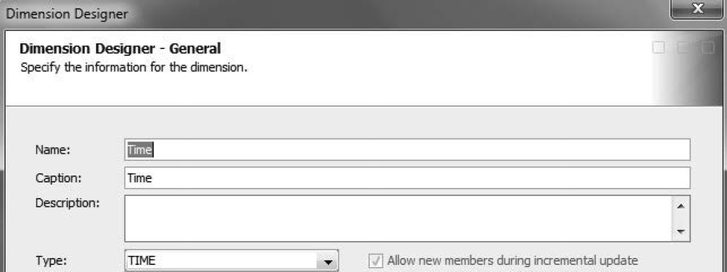
4. In the Dimension Designer wizard, create two dimensions. Start with the Time dimension.
There are three dimension types in SAS OLAP Cube Studio. These are Time, Geo, and Standard. Time enables you to create time-specific variables with a date variable. Geo creates a GIS or Geography dimension. Standard is used for all other categorical dimensions.
a. On the General page, select TIME as Type.
Figure 4.3: Create a Time Dimension
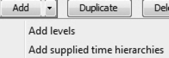
b. For Level, select Add → Add supplied time hierarchies. This is a handy shortcut for getting SAS to create various time variables from a specified date variable.
Figure 4.4: Add Supplied Time Hierarchies
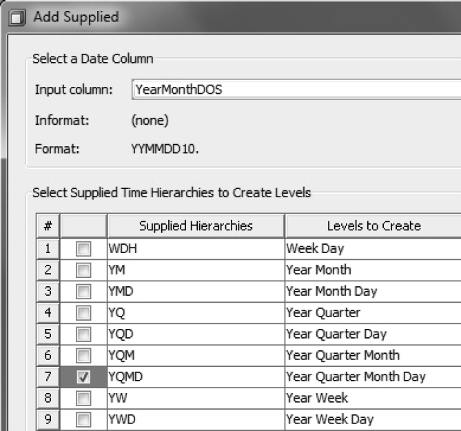
c. In the Add Supplied dialog box, select YearMonthDOS as the input column and the YQMD hierarchy to create the Year, Quarter, Month, and Day variables or levels.
Figure 4.5: Select a Time Hierarchy
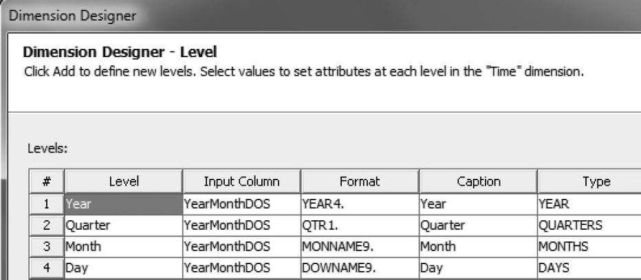
d. Verify that the dimension has been correctly created.
Figure 4.6: Time Dimension
5. Create the Type dimension. This dimension captures the encounter type (ER or Inpatient) and the associated diagnosis.
a. On the General page, select STANDARD as Type.
b. For Level, select Category and Diagnosis. Category distinguishes an ER visit from an inpatient admission. Diagnosis is a computed column. It shows ICD-9 codes for ER visits and DRG codes for inpatient admissions.
c. Verify that the dimension has been correctly created.
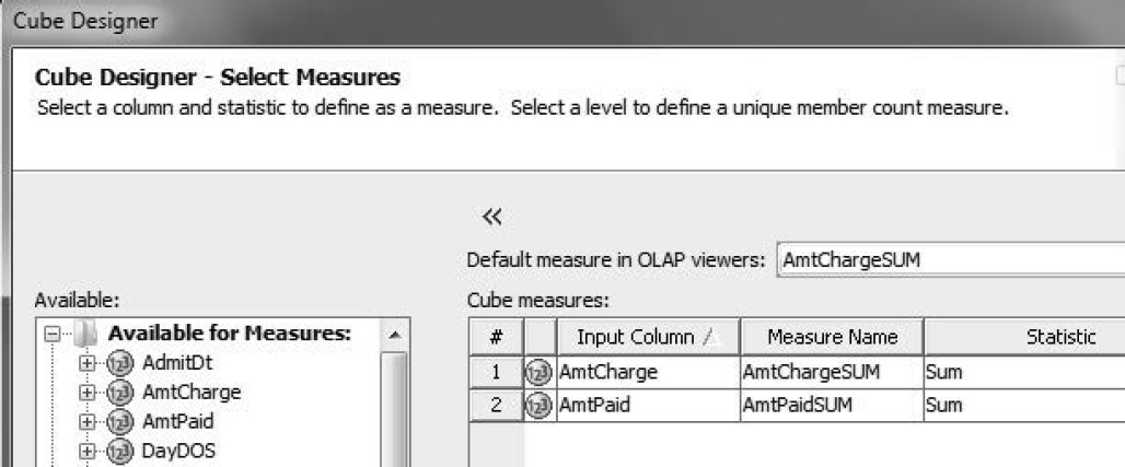
6. In the Cube Designer wizard, create measure variables in the cube. On the Select Measures page, select AmtCharge and AmtPaid.
Figure 4.7: Create Measures in a Cube
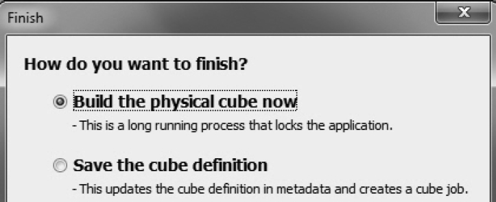
7. Click Finish to build the cube.
8. The Cube Designer wizard gives you the choice of building the cube immediately or creating a job for the cube to be built later. The latter is a good option for a large cube.
Figure 4.8: Build the Cube
9. Click Export Code on the last two pages of the Cube Designer wizard to download PROC OLAP code.
The newly created Medical Encounter Costs cube and its associated job can be found on the Folders tab of SAS OLAP Cube Studio. The job object, which appears below the cube object, can be scheduled periodically, ensuring regular data updates.
Figure 4.9 Medical Encounter Costs Cube and Its Job Object
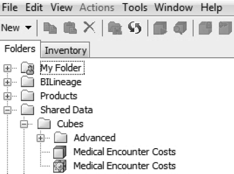
Recall that a cube is a series of files. The files for Medical Encounter Costs are stored in the physical cube path specified on the General page of the Cube Designer wizard. BI users do not need to concern themselves with the physical location of the files. They access the cube from the Shared Data/Cubes folder, and they can assume that this is where the cube is located. SAS programmers should note that Shared Data/Cubes is the metadata manifestation of the cube.
4.3.2 Adding Calculated Items to the Cube
This section adds a computed item–the paid/charged amounts ratio–to the cube.
Monitoring the paid/charged amounts ratio and its components is important to health insurance companies. This is because they often contract with providers to pay a fixed percentage of charges.
1. Click Medical Encounter Costs on the Folders tab.
2. Select Calculated Members from the Actions menu.
3. In the New Member dialog box, select Simple Calculations.
4. In the Simple Calculations dialog box, select Ratio, and select a numerator and denominator.
Figure 4.10: Add Computed Items to a Cube
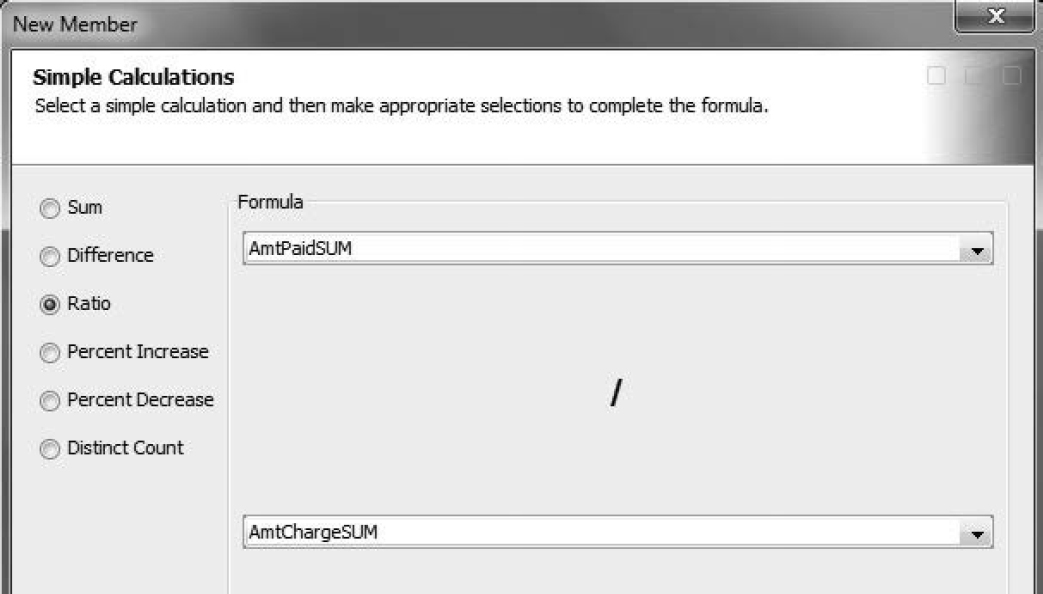
5. Format the calculation and verify the computed item.
4.4 Using OLAP Cubes with SAS Add-In for Microsoft Office
This section uses a task-oriented approach to conduct an OLAP analysis in Excel with SAS Add-In for Microsoft Office.
1. To open the Medical Encounter Costs cube, click SAS Data in the SAS ribbon.
2. Select the cube as shown in Figure 4.11.
a. Click Browse to navigate and select a cube.
b. Select SAS OLAP Analyzer.
Figure 4.11: Open a Cube in Excel
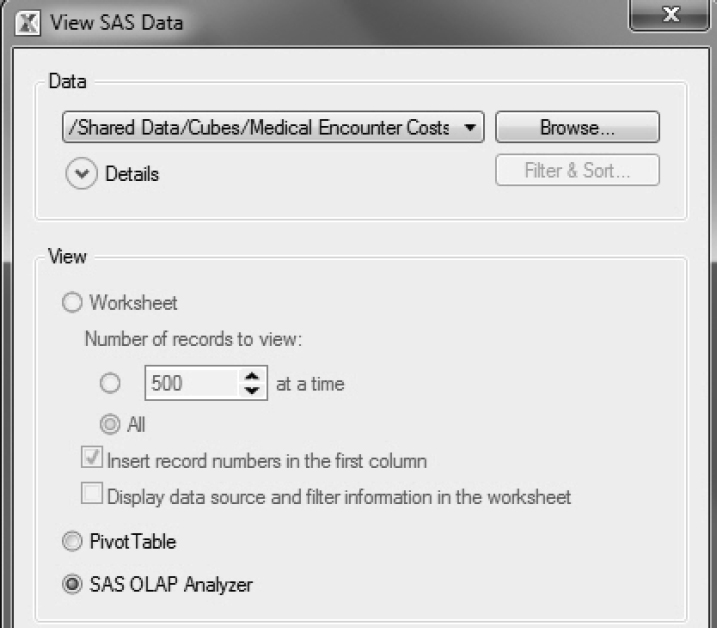
1. Filter & Sort is grayed out because a cube cannot be filtered at this stage.
2. Pivot Table opens the OLAP cube as an Excel pivot table.
4.4.1 Essentials of the SAS OLAP Analyzer
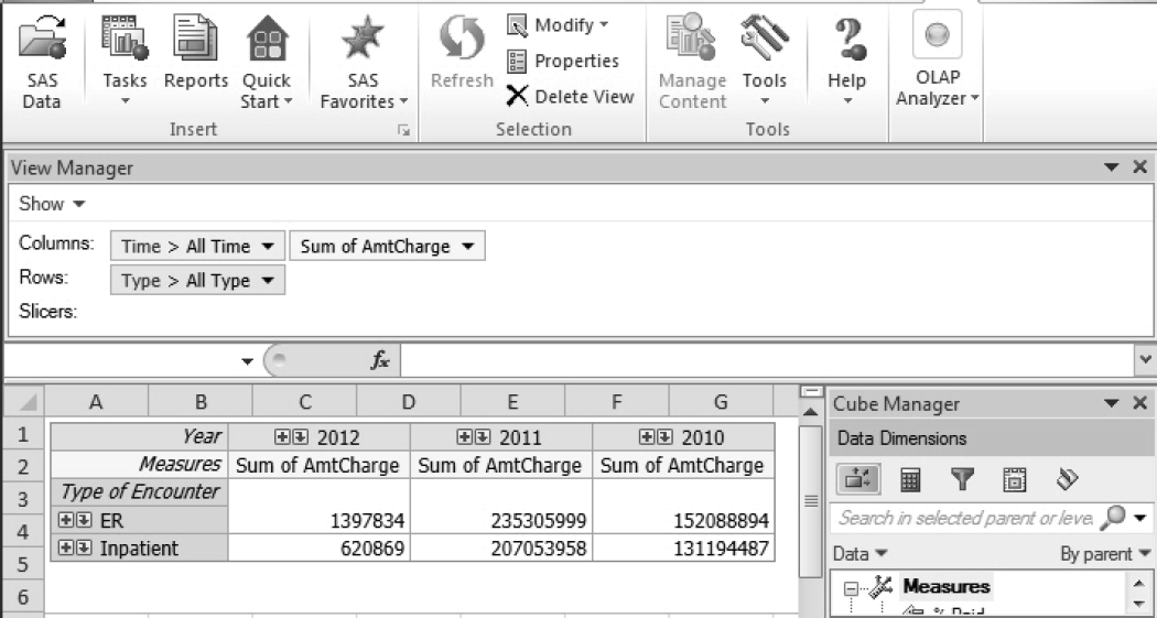
1. A default view of the Medical Encounter Costs cube opens in the SAS OLAP Analyzer. This is shown in Figure 4.12.
a. The Cube Manager customizes a cube view. Its various tabs help you place filters, create new measures, and highlight data.
b. The View Manager shows the current configuration of the cube.
c. The cube data is placed in the worksheet. In this book, this is referred to as the cube view.
Figure 4.12: Elements of the SAS OLAP Analyzer
In the SAS ribbon, OLAP Analyzer has some useful icons.
![]() Creates a graphical cube view rather than the default tabular cube view.
Creates a graphical cube view rather than the default tabular cube view.
![]() Exports OLAP data to an Excel worksheet.
Exports OLAP data to an Excel worksheet.
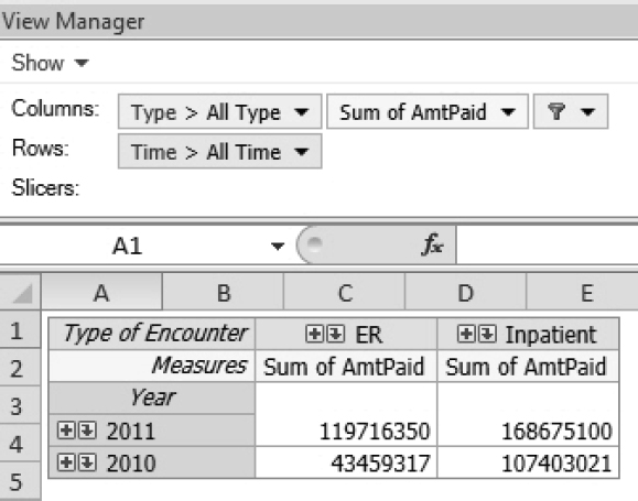
4.4.2 Adding Measures and Moving Dimensions
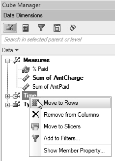
Task: Move Time to the row space of the cube.
In the Cube Manager, right-click Time on the Data Dimensions tab, and select Move to Rows.
Figure 4.13: Move Time to Row Space
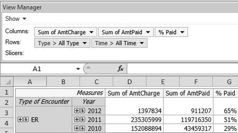
Task: Add measure variables to the column space of the cube.
The Data Dimensions tab of the Cube Manager contains a folder for each dimension. Measures are clustered in the Measures dimension by default.
1. On the Data Dimensions tab, right-click Sum of AmtCharge, and select Move to Columns.
2. % Paid can be moved to the column space in two ways. It is a computed item, so it is on the Data Dimensions tab and Customized Items and Sets tab. Right-click % Paid from either tab, and select Move to Columns.
3. View Sum of AmtCharge and % Paid in the cube view.
Figure 4.14: Customize a Cube View
4.4.3 Slicing and Dicing in the SAS OLAP Analyzer
This section presents two essential OLAP functionalities. These are drilling in and drilling out of a dimension and expanding and collapsing data along a dimension.
Task: Drill in and drill out of a dimension.
Begin with a simplified view of the cube.
Figure 4.15: Drill In and Drill Out
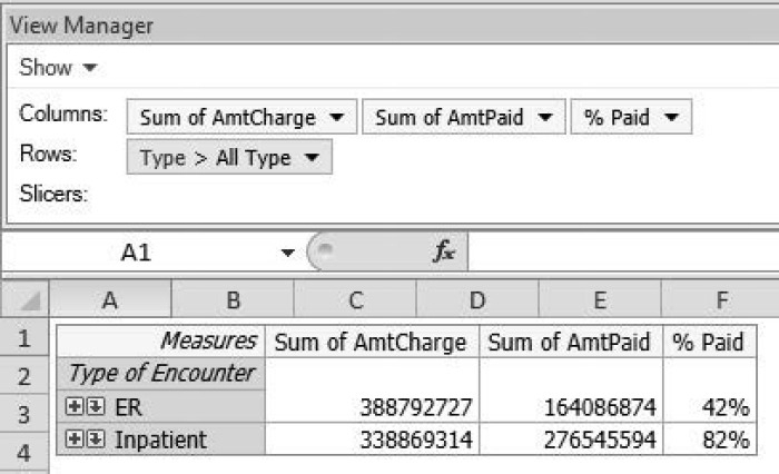
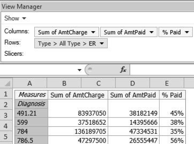
1. In the View Manager, Type is displayed as a link. It is followed by the icon. This icon means that the dimension has been drilled into. To drill out, click Type. The results are shown in Figure 4.16.
Figure 4.16: Drill Out in the View Manager
2. To drill into a dimension, click on the down arrow to the left of All Type in the cube view.

3. When a dimension has been drilled into, its preceding levels are hidden. In Figure 4.17, the Type dimension has been drilled into completely.
Figure 4.17: Drill Into a Dimension
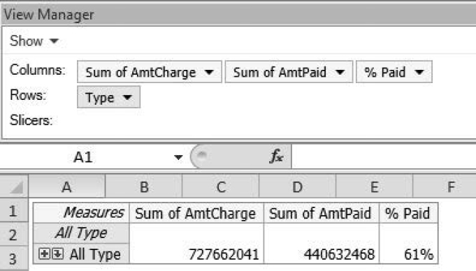
4. To drill out once, click All Type in the View Manager.
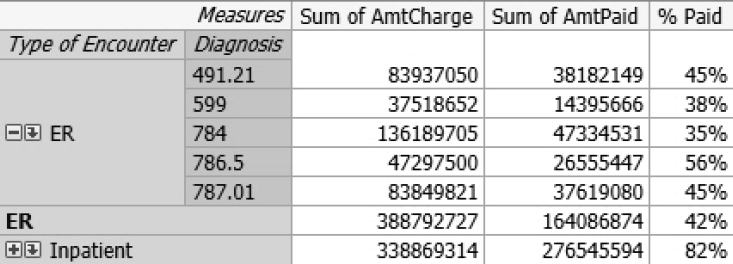
Task: Expand and collapse data along a dimension.
The concept of expanding and collapsing data is similar to drilling in and drilling out. As you expand data, you traverse down the hierarchy into a lower level of the dimension, but you continue to see the previous level. As you collapse data, you navigate up the hierarchy into a higher level of the dimension.
1. To expand ER, click on the plus sign to the left of ER in the cube view ![]() .
.
2. ER is expanded to its next level, Diagnosis, in the dimension. Notice the negative sign to the left of ER. If you click the negative sign, the data collapses Diagnosis.
Figure 4.18: Expanding and Collapsing Dimensions
4.4.4 Filtering and Slicing
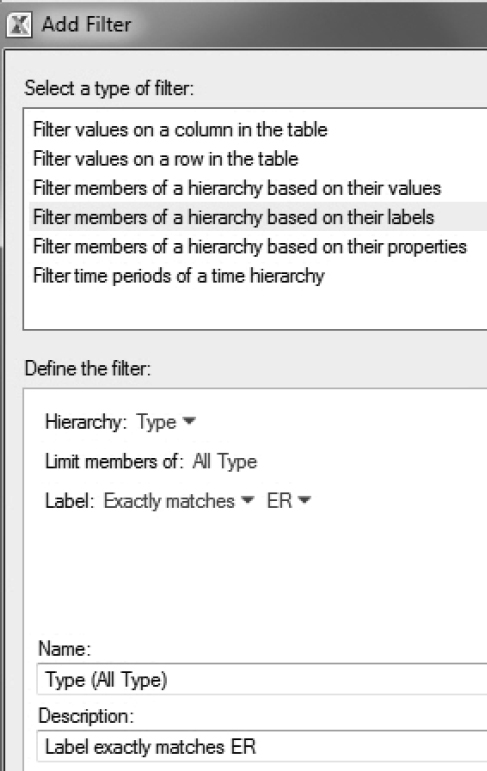
Task: View ER visits only.
1. In Cube Manager, click the Filters icon  .
.
2. In the Add Filter dialog box, select Filter members of a hierarchy based on their labels, and enter ER for Label.
Figure 4:19: Add a Filter
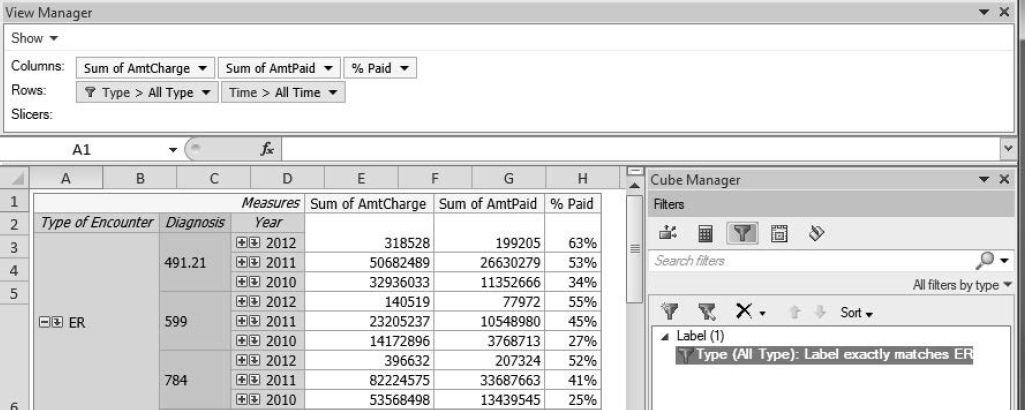
3. Right-click on the new ER filter on the Filters icon, and select Add to View.
4. View ER visits only.
Figure 4.20: Filter Results in a Cube
Task: Find time periods where AmtPaid for ER visits equals or exceeds $1 million.
1. On the Filters tab in the Cube Manager, clickxs Filter .
2. In the Add Filter dialog box, select Filter values on a column in the table.
3. As shown in Figure 4.21, define the filter, and select Range for Based on.
Figure 4.21: Filter the Cube
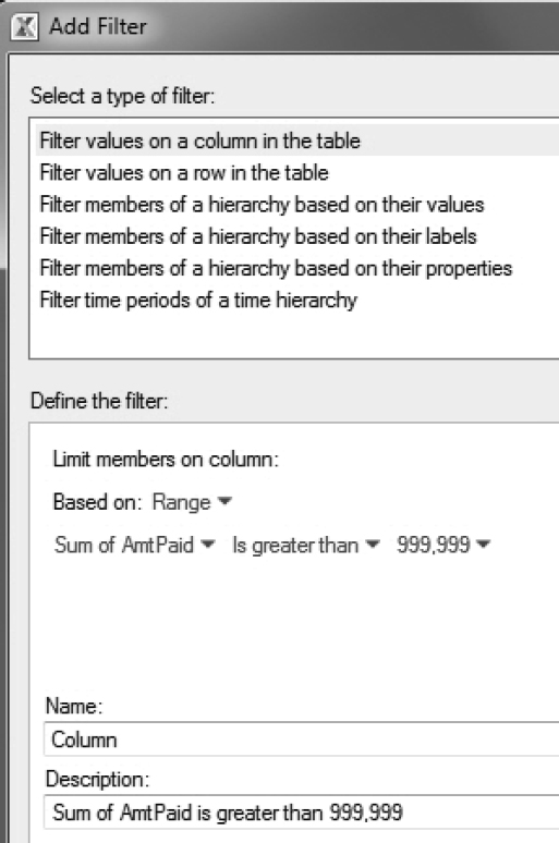
4. Confirm the results. The filter enables users to see only time periods where paid amounts for ER visits equal or exceed $1 million. The year 2012 is not shown because Healthy Living Inc. paid less than $1 million for ER visits in 2012.
Figure 4.22: Filter Results in a Cube
At any stage of analysis, the Excel workbook can be saved and closed. To get back to the SAS OLAPAnalyzer, simply reopen the workbook, and click Activate OLAP Analyzer.
Task: View visits from 2011 only.
Although this task can be done using filtering, it is important to demonstrate the functionality of the Slicers row in the View Manager. A slice of 2011 data is a segment of the cube where the following is true:
• Year is held constant at its value of 2011.
• The Time dimension is no longer shown.
1. While Time is drilled into for 2011, use the drop-down menu for Time in the View Manager, and select Move to Slicers. This is shown in Figure 4.23.
Figure 4.23: Use Slicers
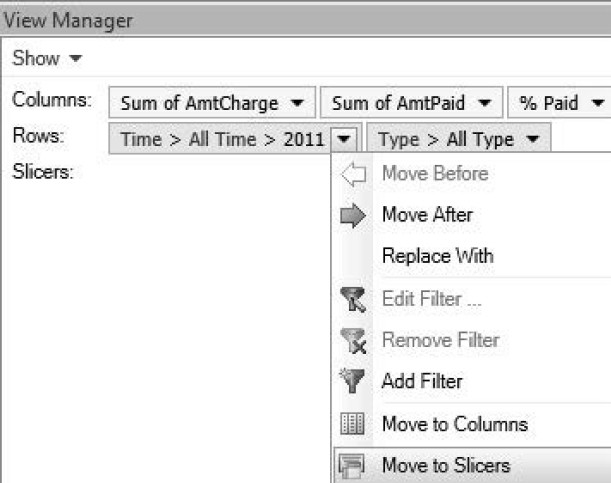
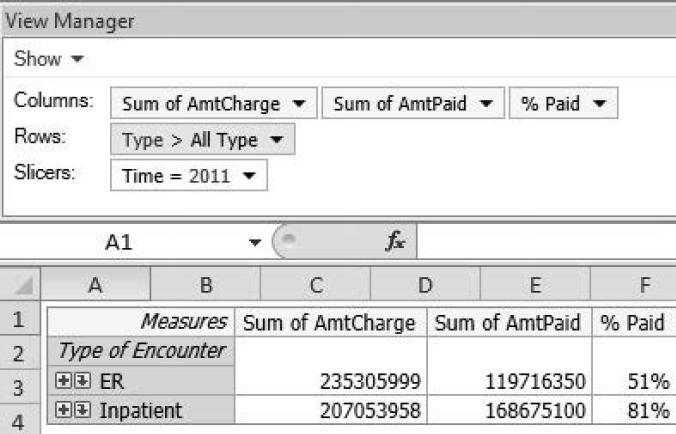
2. View the results. Time is shown in the Slicers row and no longer plays a role in the cube view.
Figure 4.24: A Cube Slice
4.4.5 Creating Computed Measures
Task: Compute percent of total charged amount.
1. On the Customized Items and Sets tab of the Cube Manager, click Add, and select Percent of Visual Total as shown in Figure 4.25. The visual total does not need to be the same as the total in the cube, especially when there are filters or slices.
Figure 4.25: Add Total to Cube View
2. Totals come in many flavors. There are grand totals, row totals, and column totals. Select Grand Total.
Figure 4.26: Grand Total in Cube View
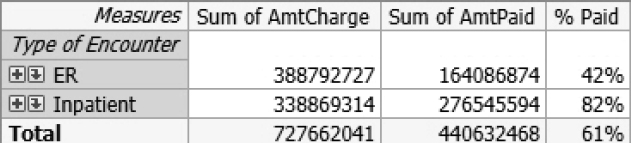
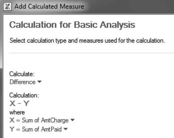
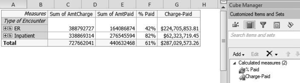
Task: Compute the differences between the charged and paid amounts.
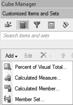
1. On the Customized Items and Sets tab of the Cube Manager, click Add, and select Calculated Measure.
2. In the Add Calculated Measure dialog box, choose Basic analysis.
3. Create the calculation as shown in Figure 4.27.
Figure 4.27: Computed Items in the Cube View
4. Verify the results.
Figure 4.28: Computed Items in the Cube View and Cube Manager
Task: Compute rolling sums of paid amount.
Like other time series data, health-care utilization has seasonal components. For example, it tends to spike during the flu season. This seasonality can be removed by taking an average or total of the last several periods of data.
1. On the Customized Items and Sets tab of the Cube Manager, click Add, and select Calculated measures.
2. In the Add Calculated Measure dialog box, select Special analysis → Time series analysis.
Figure 4.29: Use Time Series Analysis
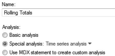
3. Create rolling totals as shown in Figure 4.30.
a. Select Rolling totals for Calculate.
b. Select Sum of AmtPaid for With measure.
c. Select 2 under Number of periods from current. This includes the current and previous periods.
Figure 4.30: Create Rolling Totals
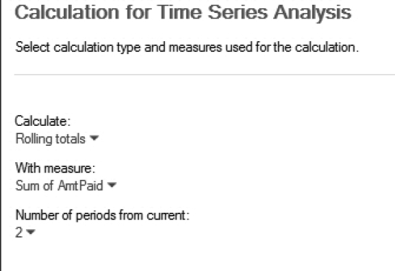
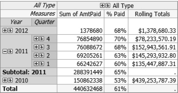
4. Verify that the rolling totals include current and previous periods.
Figure 4.31: View Rolling Totals in the Cube View
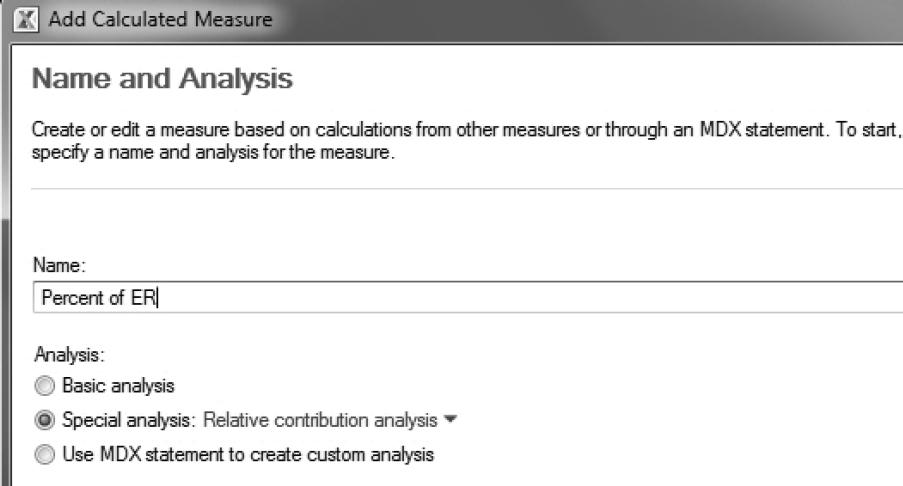
Task: Identify the major components of ER expenditures.
1. On the Customized Items and Sets tab of the Cube Manager, click Add, and select Calculated measures.
2. In the Add Calculated Measure dialog box, select Special analysis → Relative contribution analysis.
Figure 4.32: Relative Contribution Analysis
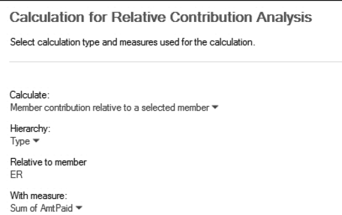
3. The objective is to connect amount paid for ER to any amount in Type. Enter information as shown in Figure 4.33.
a. Select Type for Hierarchy. This is the numerator.
b. Select ER for Relative to member. This is the denominator.
Figure 4.33: Type Dimension as Percentage of ER
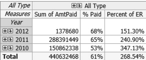
4. In Figure 4.34, Percent of ER shows ER as a percentage of the total amount paid.
Figure 4.34: Type as Percent of ER
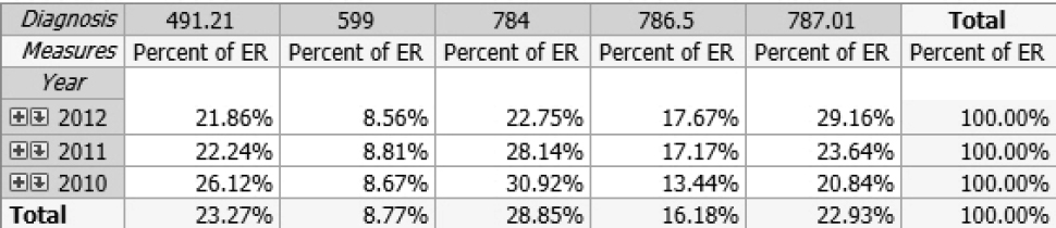
5. Percent of ER is useful when the cube is drilled into the Diagnosis level. Figure 4.35 shows the impact of each diagnosis on ER paid amounts.
Figure 4.35: Diagnosis as Percent of ER
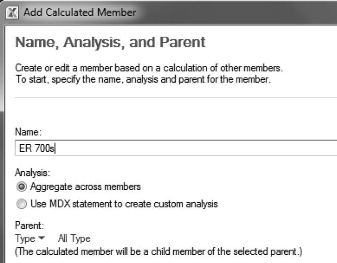
Task: Group diagnosis codes in the 700s range together.
1. On the Customized Items and Sets tab of the Cube Manager, click Add, and select Calculated member.
2. Select Aggregate across members. Select Type as the Parent dimension.
Figure 4.36: Group Diagnosis Codes
3. Select diagnoses to group.
Figure 4.37: Group Diagnosis Codes
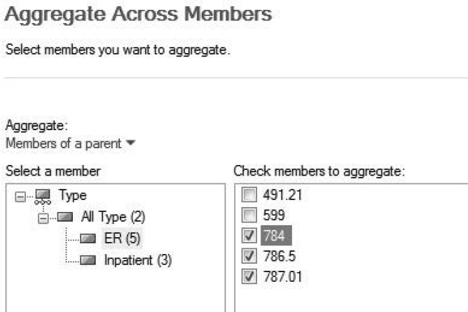
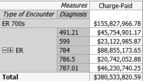
4. Verify the grouping in the results.
Figure 4.38: Create New Diagnosis Groups
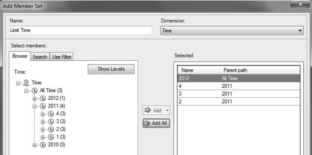
Task: Limit data to the entire year of 2012 and the last three quarters of 2011.
1. On the Customized Items and Sets tab of the Cube Manager, click Add, and select Member Set.
2. In the Add Member Set dialog box, select time periods as shown in Figure 4.39.
Figure 4.39: Limit across Time Hierarchy
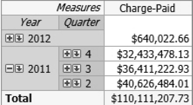
3. Verify the results.
Figure 4.40: Limit across Time Hierarchy
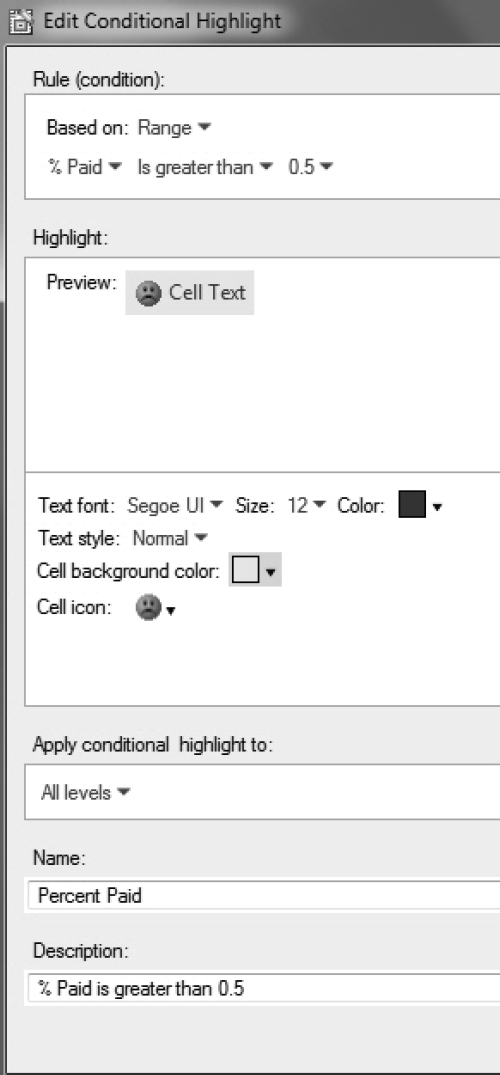
4.4.6 Conditional Highlighting
Task: Highlight rows where percent paid exceeds 50%.
1. On the Conditional Highlights tab in the Cube Manager, click  . This icon creates a new highlighting rule.
2. Create the highlighting rule as shown in Figure 4.41. Select All levels in Apply conditional highlight to to apply the rule to all levels in the Type dimension.
Figure 4.41: Create a Highlighting Rule
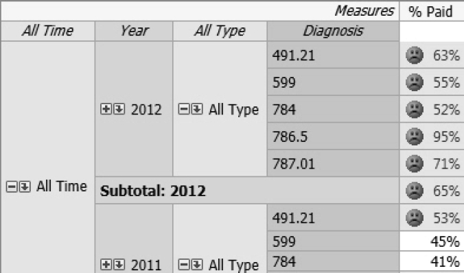
3. The highlighting rule is applied in Figure 4.42.
Figure 4.42: Highlight High Percent Paid
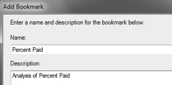
4.4.7 Bookmarking a Customized Cube View
Task: Save the cube view so that it is available for future use.
1. On the Bookmarks tab in the Cube Manager, click  . This icon creates a new bookmark.
When a cube is opened using SAS Add-In for Microsoft Office, it creates a default bookmark called Initial view, which cannot be removed.
2. In the Add Bookmark dialog box, enter the name of the bookmark.
Figure 4.43: Add a New Bookmark
3. The new bookmark is shown in Figure 4.44.
Figure 4.44: Bookmarks in the Cube Manager
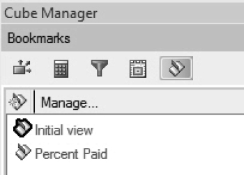
If a computed item that is being used in a bookmark is deleted, then the bookmark is deleted as well.
4.5 Conclusion
This chapter taught you how to create a basic cube using SAS OLAP Cube Studio. It showed you how to leverage the vast capabilities of SAS Add-In for Microsoft Office to effectively analyze cube results and create your own custom views of the cube.