
Chapter 8: Advanced OLAP Applications in the Health-Care Industry
8.2 Creating a Multipurpose Cube
8.2.1 Creating a Star Schema Cube in OLAP Cube Studio
8.2.2 Building an OLAP Information Map
8.2.3 Creating Multi Sectioned Reports in Web Report Studio
8.3 Implementing OLAP Data Security via MDX
8.3.1 Fundamentals of OLAP Concepts and Terminology
8.3.2 Creating MDX Expressions with Enterprise Guide
8.3.3 Restricting Data Access with MDX
8.4 Computing Healthcare Metrics in an OLAP Cube
8.4.3 Creating an OLAP Cube from Summary Tables
8.1 Introduction
This chapter describes three advanced OLAP web applications in the health-care industry. Although the chapter’s primary focus is on SAS OLAP Cube Studio, it also covers pertinent features of SAS Web Report Studio and SAS Information Map Studio. Here is some background information about the three applications featured in this chapter.
Application 1: Most health-care organizations reorganize their transactional data into a data warehouse for analytical purposes. The data warehouse usually consists of key fact or transactional tables, surrounded by dimensional or lookup tables. This design is referred to as a star schema. The data mart at Healthy Living Inc. is a star schema. It consists of a key fact table named Encounter, surrounded by various dimensional tables. See Figure 1.1 in Chapter 1, “An Overview of SAS Business Intelligence,” for more information.
The first OLAP application extends the Medical Encounter Costs cube created in Chapter 4, “Slicing and Dicing Data with OLAP Cubes,” to encompass Healthy Living Inc.’s star schema data mart. The cube is used to develop a number of SAS Web Report Studio reports, each catering to the analytical needs of a different department at Healthy Living Inc.
Application 2: HIPPA privacy rules impose data access restrictions on health-care organizations. Chapter 7, “Data Security and Dynamic Updates with SAS Information Map Studio,” showed programmers how to implement data security in information maps based on relational data. This application describes how data access restrictions are implemented in an OLAP cube. The application includes an OLAP web report that allows each claim representative to view only his or her own claims.
MDX, the multidimensional equivalent of SQL, is used to build expressions that restrict data access intelligently. MDX is a difficult language to learn because its syntax represents OLAP concepts often unfamiliar to the SAS programmer. As a learning strategy, the fundamentals of these OLAP concepts and MDX syntax conventions are presented first. Then, SAS Enterprise Guide is used to create some basic MDX code. This preparatory work enables programmers to write complex expressions required for data security.
Application 3: Health-care organizations measure outcomes and utilization on a per patient basis. However, the unit of analysis in health care is a patient encounter or service. Metrics such as cost per member per month cannot be added across services. To understand the challenge this poses, consider the simple scenario described in Table 8.1.
Table 8.1: Aggregation Challenges in Health-Care Data
| Type of Service | Number of Visits | Number of Enrolled Members | Utilization Per Member |
| Primary Care Visits | 10 | 50 | .2 |
| ED Visits | 10 | 50 | .2 |
| Incorrect Member Total | 20 | 100 | .2 |
| Correct Total | 20 | 50 | .4 |
Although the number of visits is additive across types of service, the number of enrolled members is not. This is because the total number of enrolled members is 50, not 100. The third application uses summary data sets to correctly compute metrics.1
8.2 Creating a Multipurpose Cube
Healthy Living Inc. has a data mart in the form of a star schema. Encounter is the company’s primary fact table. The fact table can be combined with dimensional tables to provide additional insight into medical encounters.
In this section, you accomplish the following:
1. Create a multipurpose cube using Healthy Living Inc.’s star schema data mart.
2. Build an OLAP information map with simple and prompted filters.
3. Create a multi-sectioned SAS Web Report Studio report. Providing comparative analytics, this report is useful to multiple departments in the company.
8.2.1 Creating a Star Schema Cube in SAS OLAP Cube Studio
Here is a quick review of key OLAP concepts:
1. A cube examines key metrics with respect to slicer variables. Paid and charged amounts are examples of metrics or measures.
2. Slicer variables are grouped logically into buckets called dimensions.
3. A dimension generally contains several variables that are called levels.
4. The ordering of levels in a dimension is called hierarchy.
Because cube creation using SAS OLAP Cube Studio has been covered in Chapter 4, only new material is discussed in this chapter. Now, create a star schema cube in SAS OLAP Cube Studio.
1. On the Cube Designer - General page, select Star schema as Input Type. This sources a cube from a data mart rather than from a single table.
2. On the Cube Designer - Input page, move Encounter to Fact table.
3. On the Cube Designer - Dimensions page, move ClaimRep, Provider, and Demographics to Selected tables.
4. Create dimensions and measures listed in Table 8.2.
Table 8.2: Star Schema Cube
| Dimension Name | Levels in Hierarchy | |
|---|---|---|
| Dimension | Claims Rep | Tenure, Sex, Name |
| Demographics | ZIP code, Plan, Sex | |
| Provider Type | Provider Type, Name | |
| Time | Year, Quarter, Month | |
| Type | Category, Diagnosis | |
| Measure | Measures | Amount Charged, Amount Paid (Sum) |
5. Create a cube named Medical Encounters Adv.
8.2.2 Building an OLAP Information Map
In this section, you create an OLAP information map with a computed item and simple and prompted filters.
1. On the Server tree tab of the Resources - Application Servers dialog box, select Cubes from the Show menu. Add Medical Encounters Adv to Selected Resources as shown in Figure 8.1.
Figure 8.1: Source an Information Map from a Cube

An OLAP information map allows only one cube as its data source. This is why the Relationship tab does not appear.
Compound filters or filters based on more than one data item are not allowed in OLAP information maps.
2. Create Percent Paid, a computed item in the map, as a ratio of amount paid to amount charged. See section 5.3.5, “Creating Computed Items,” for more information.
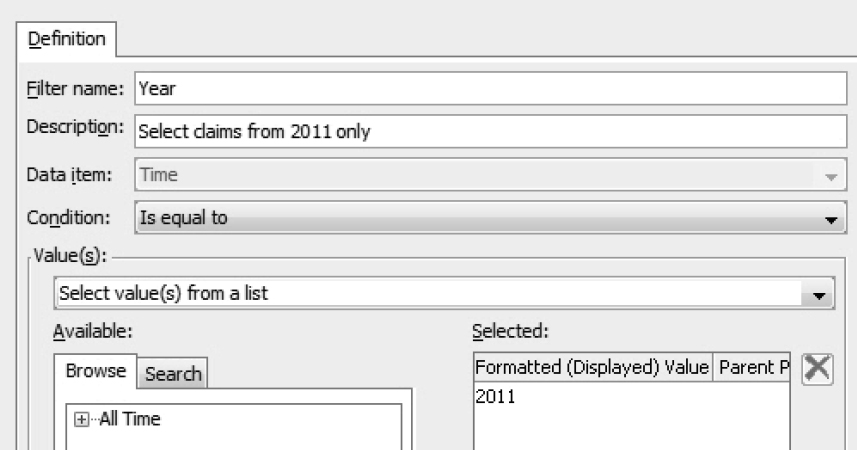
3. Build a filter using Year to include only medical claims from 2011.
Figure 8.2: Filtering in an OLAP Information Map
4. Build prompted filters for Provider, ZipCode, and Claims Rep. These filters enable a single report to be used by multiple departments. See section 5.3.6, “Creating Filters,” for more information.
a. Click the New Filter icon.
b. In the New Filter dialog box, enter the following information:
i. Value(s): Select Prompt user for value(s).
ii. Click New to create a prompt for Provider.
c. On the General tab of the New Prompt dialog box, enter the following information:
i. Name: Name of the prompt.
ii. Displayed text: Text with which the user is prompted.
d. On the Prompt Type and Values tab of the New Prompt dialog box, enter the following information as shown in Figure 8.3:
i. Number of values: Select Multiple values.
ii. Data Item: Select Provider Type.
Figure 8.3: Create a Prompt in an OLAP Information Map

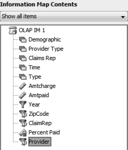
5. Verify the filters from the Information Map Contents dialog box
Figure 8.4: Information Map Contents
8.2.3 Creating Multi-Sectioned Reports in SAS Web Report Studio
The health-care industry relies heavily on comparative analytics to identify potential areas of improvement. A health insurance company might examine key metrics across demographic areas to identify outlier areas. It might compare physician or clinic performance.
Comparative analytics play an important role in several departments at Healthy Living Inc. The Provider Services department compares hospital costs. The Claims department compares the performance of claims representatives. The Medical Management department compares health-care costs and utilization across demographic areas.
In this section, you use an information map to create a multi-sectioned report. You build a report section comparing Healthy Living Inc.’s hospitals. This is used as a template for other comparative analytics, making the entire report applicable to multiple departments in the company.
No comparative study in health care is valid before you account for differences in population groups. For example, you cannot compare the costs and utilization of children to the costs and utilization of the elderly. To compare disparate populations, you need to adjust their usage and costs. This is known as risk adjustment. Because risk adjustment is beyond the scope of this book, the focus is on a simplified comparative analysis.
1. Create a new report in SAS Web Report Studio. See section 6.4, “The Basics of SAS Web Report Studio.”
2. Select the OLAP information map created in the previous section (OLAP IM 1) as the data source.
Figure 8.5: Select a Data Source
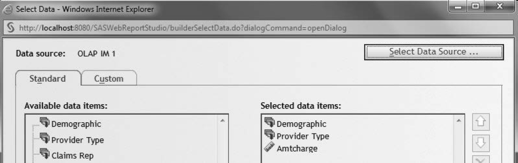
The Custom tab in the Select Data dialog box enables the programmer to create computed items in SAS Web Report Studio. However, computed items and filters should be placed in the information map where they can be shared by multiple reports.
3. On the Edit tab, create a report as shown in Figure 8.6.
a. Drag and drop a tabular report object and a graph report object onto the reporting slate.
b. Create a report header and footer.
c. Select Options → Rename Section to rename the report section.
Figure 8.6: Create Provider Comparison Report

4. Select Data → Section Filters, and select Provider to apply the filter.
Figure 8.7: Apply Prompted Filter in SAS Web Report Studio
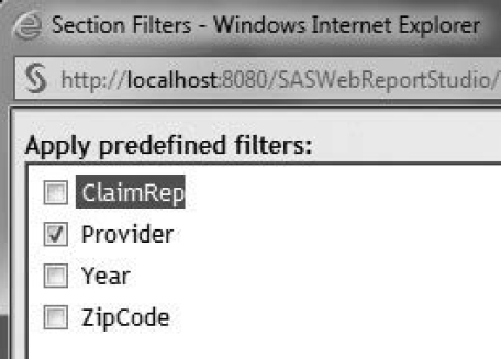
SAS Web Report Studio allows programmers to choose more than one prompted filter in a report. Manage Prompts in the Section Filters dialog box allows programmers to determine the order in which the prompted filters are presented to the user.
5. Right-click on the tabular report object, and select Assign Data. Assign data items as shown in Figure 8.8.
Figure 8.8: Assign Data in SAS Web Report Studio

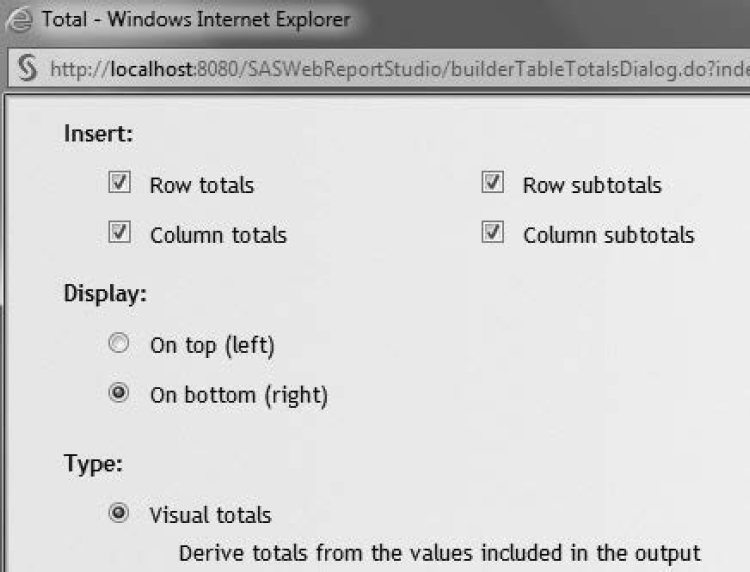
6. Insert totals in the report by right-clicking on the tabular report object, and then selecting Totals. Select totals and display options.
Visual totals computes totals from the data pulled into the report, rather than from the data in the information map.
Figure 8.9: Insert Totals in SAS Web Report Studio
7. Right-click on the graph report object, and select Assign Data. Assign data items as shown in Figure 8.10.
Figure 8.10: Assign Data in SAS Web Report Studio

8. Click the View tab. Select Hospital B and Hospital C when prompted.
9. The following conclusions can be made from the tabular report. You can further expand or drill into the Time and Type dimensions.
a. Hospital C received $245 million over the three-year period from Healthy Living Inc. Hospital B received $140 million over the same three-year period.
b. Paid amounts as a Percent Paid of Charge amounts are increasing across time from 53% in 2010 to 65% in 2012.
c. Hospital B receives a higher percent of payments for ER services than Hospital C. The exact opposite is true for Inpatient services.
Figure 8.11: Provider Comparison Report

10. The following bar chart confirms the findings of the tabular report. You can further expand or drill into the Time and Type dimensions. To view the diagnosis codes in ER encounters, right-click ER, and select Drill Down on ER. To drill into the Time dimension, right-click on a bar (each one represents a year of data).
Figure 8.12: Provider Comparison Report
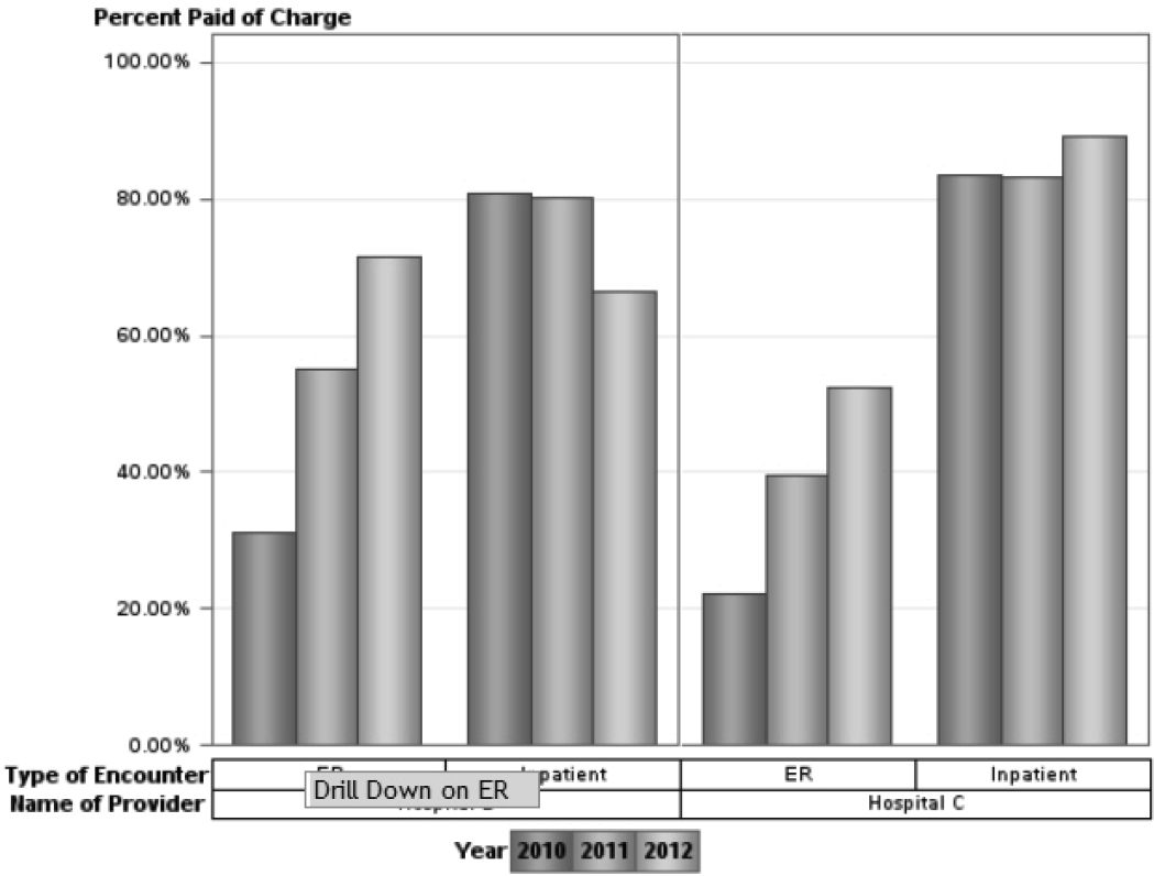
The report helps the Provider Services department track payments, monitor contracts, and correct payment errors. The drill-down capability of the report helps analysts identify specific areas of high payments. This knowledge is particularly relevant to Healthy Living Inc. during contract negotiations with hospitals.
The Provider Comparison Report is used as a template to build the remaining reports.
1. On the Edit tab, select Options → Copy Section to copy the Provider Comparison Report.
2. Repeat steps 5 through 7 to build the ZipCode Comparison report.
3. Apply the ZipCode prompted filter to the report.
4. View the report.
Figure 8.13: ZipCode Comparison Report

The ZipCode Comparison report is used by the Medical Management department at Healthy Living Inc. The drill-down capability of the report helps analysts identify specific areas of high cost. A quick perusal of the tabular report reveals that Healthy Living Inc. spends almost twice as much in ZIP code 97229 as it does in ZIP code 97005.
5. Repeat steps 1 through 2 to build the Claims Representatives Comparison report.
6. Apply the ClaimRep filter to the report.
7. View the report.
The Claims Representatives Comparison report enables the Claims department at Healthy Living Inc. to compare the work performance of two or more claims representatives.
Figure 8.14: Claims Representatives Comparison Report

8.3 Implementing OLAP Data Security via MDX
In this section, you create an OLAP application that allows each claims representative at Healthy Living Inc. to view only his or her own claims. This is accomplished with a security expression in an OLAP cube using MDX, the multidimensional equivalent of SQL.
Learning MDX is often a challenge because it contains new OLAP concepts, terminology, and syntax. To facilitate learning, this section is divided into three parts. First, the fundamentals of OLAP concepts and MDX syntax conventions are presented. Next, SAS Enterprise Guide is used to generate and understand basic MDX code. Finally, complex conditions required for security are created.
For the purpose of simplicity, a pared-down version of the multipurpose cube created in the previous section is used. Based on a star schema, the new cube uses Encounter as its fact table and ClaimRep as its sole dimensional table. To keep things simple, the ClaimRep dimension contains only the name of the claims representative.
Table 8.3: Characteristics of Claim Rep Data Security Cube
| Dimension Name | Levels in Hierarchy | |
|---|---|---|
| Dimension | Claim Rep | Name |
| Time | Year, Quarter, Month | |
| Type | Category, Diagnosis | |
| Measure | Measures | Amount Charged, Amount Paid (Sum) |
8.3.1 Fundamentals of OLAP Concepts and Terminology
Here are some familiar and new OLAP concepts in the context of the Claim Rep Data Security cube:
Table 8.4: A Review of OLAP Concepts
| Name | Definition | Example |
|---|---|---|
| Dimension | A logical grouping of variables | The Type dimension contains two related variables, Category and Diagnosis. |
| Hierarchy | The ordering of variables in a dimension | The hierarchy of the Time dimension is Year, Quarter, and Month. |
| Level | Variable in OLAP terminology | Category and Diagnosis are two levels of the Type dimension. SAS OLAP creates an overarching level called All, which is placed at the top of a hierarchy. |
| Measure | Metrics in an OLAP cube | Amtpaid and Amtcharge are both measures in the Measures dimension. |
| Member | A distinct value of a level | The level Category in the Type dimension has two members, Inpatient and ER. |
SAS OLAP Cube Studio presents these OLAP concepts in a format that is easily understood. This is shown in Figure 8.15 and explained in Table 8.5.
Figure 8.15: Dimensions, Hierarchies, and Levels in a Cube
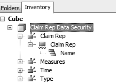
Table 8.5: OLAP Icons and Terminology
 |
The dimension has its own folder structure, indicating that it is a container for like elements. |
| The hierarchy is the order of levels in a dimension. | |
 |
Is a level in the dimension. Levels are nested inside the hierarchy. |
| Tuple | Is the location of a cell, not its value, in a cube. It is written as coordinates from the cube’s various dimensions, hierarchies, levels, and members. |
| Set | Is a collection of tuples. |
Here is some information about MDX naming conventions:
1. A dot is generally used to separate levels within a dimension. The Type dimension has two levels, Category and Diagnosis. Members of Category are Inpatient and ER. Members of Diagnosis are ICD-9 codes for ER visits and DRG codes for inpatient admissions. In pseudo MDX, Inpatient.291 refers to DRG code 291 for an inpatient admission.
2. A comma is used to separate one dimension from another. An intersection between the Time and Type dimensions is written in pseudo MDX as Inpatient.291, 2010.1.January.
3. Square brackets are generally used around cube, dimension, and member names. The example in step 2 can be rewritten more accurately as [Type].[All Type].[Inpatient].[291],[Time].[All Time].[2010].[1].[January]. A dot is used to separate dimension names and levels.
4. Braces ( ) are placed around a tuple, which are the coordinates used to identify a cell.
5. Curly braces { } are placed around a set, which is a collection of tuples.
A tuple can be defined completely or incompletely. When the tuple definition is complete, it means that every dimension in the cube has been specified. When one or more dimensions are omitted from the coordinate specification, the tuple definition is incomplete.
The following is a complete definition of a tuple from the Claim Rep Data Security cube. The cell denotes the amount paid, processed by Jason, for January 2010, for inpatient admissions whose DRG code is 291.
([Type].[All Type].[Inpatient].[291],
[Time].[All Time].[2010].[1].[January],
[ClaimRep].[All ClaimRep].[Jason],
[Measures].[All Measures].[AmtPaid])
One or more dimensions can be omitted in a tuple specification. In the previous example, the default member of the dimension is used. In the next case, the ClaimRep dimension is not specified.
([Type].[All Type].[Inpatient].[291],
[Time].[All Time].[2010].[1].[January],
[Measures].[All Measures].[AmtPaid])
In this case, MDX completes the tuple definition, substituting the default definition of ClaimRep. The complete tuple definition refers to the amount paid, processed by all claims representatives, for January 2010, for inpatient admissions with a DRG code of 291:
([Type].[All Type].[Inpatient].[291],
[Time].[All Time].[2010].[1].[January],
[ClaimRep].[All ClaimRep],
[Measures].[All Measures].[AmtPaid])
Here is an example of a set, which is a collection of 0 or more tuples:
{
([Type].[All Type].[Inpatient].[291],
[Time].[All Time].[2010].[1].[January], (1)
[ClaimRep].[All ClaimRep].[Jason],
[Measures].[All Measures].[AmtPaid]),
([Type].[All Type].[Inpatient].[291], (2)
[Time].[All Time].[2010].[1].[January],
[ClaimRep].[All ClaimRep].[Renu],
[Measures].[All Measures].[AmtPaid])
}
1. This cell denotes the amount paid, processed by Jason, for January 2010, for inpatient admissions with a DRG code of 291.
2. This cell denotes the amount paid, processed by Renu, for January 2010, for inpatient admissions with a DRG code of 291.
8.3.2 Creating MDX Expressions with SAS Enterprise Guide
In this section, you use the point-and-click interface in SAS Enterprise Guide to generate MDX code for two measures. This code is then copied and pasted in SAS OLAP Cube Studio.
The first computed item, Percent of ER Paid, is instrumental in auditing and trending analysis. The second computed item, Rolling Total of Paid Amount, is useful because it levels out seasonal variations in health-care utilization and costs.
Percent of ER Paid
1. Open the Claim Rep Data Security cube in SAS Enterprise Guide using File → Open → OLAP Cube.
2. On the Customized Items and Sets tab, click Add, and select Calculated Measure.
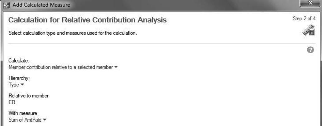
3. Select Special Analysis-Relative Contribution Analysis.
4. Benchmark Sum of AmtPaid in the Type hierarchy to Sum of AmtPaid for ER as shown in Figure 8.16.
a. Select Type for Hierarchy. This is the numerator.
b. Select ER for Relative to member. This is the denominator.
Figure 8.16: Relative Contribution Analysis
5. Examine and copy the MDX expression from Summary.
(a) Create Member
(b) [Claim Rep Data Security].[Measures].[Percent of ER Paid] AS
(c) ([Measures].[AmtPaidSUM],[Type].[Type].CurrentMember)
/
(d) ([Measures].[AmtPaidSum], [Type],[All Type].[ER])
a. Create a statement in MDX to create a measure or member.
b. The new measure, Percent of ER Paid, is located in the Measures dimension.
c. The numerator includes the current cell in the Type dimension. The CurrentMember function retrieves the current tuple or cell coordinates.
d. The denominator includes AmtPaidSum for ER.
6. Add the MDX expression from step 5 to the cube definition.
a. In SAS OLAP Cube Studio, select Actions → Calculated Members.
b. Select Custom Calculations.
c. Paste only the formula portion of the MDX expression from step 5.
([Measures].[AmtPaidSUM],[Type].[Type].CurrentMember)
/
([Measures].[AmtPaidSum], [Type],[All Type].[ER])
7. Verify the Percent of ER Paid in SAS Enterprise Guide. The new measure works even when dimensions are added. For example, Figure 8.17 shows how managers at Healthy Living Inc. monitor and trend the work distribution of claims representatives.
Figure 8.17: Work Distribution of Claims Representatives

Rolling Total of Paid Amount
1. Open the Claim Rep Data Security cube in SAS Enterprise Guide using File → Open → OLAP Cube.
2. On the Customized Items and Sets tab, click Add, and select Calculated Measure.
3. Select Special Analysis-Time Series Analysis.
4. In step 2 of Add Calculated Measure, enter information as shown in Figure 8.18.
a. For Calculate, select Rolling totals.
b. For With measure, select Percent of ER Paid.
c. For Number of periods from current, select 2. The computation aggregates AmtPaid from current and previous periods. The verbiage is slightly misleading, so it is best to remember that the number selected includes the current period.
Figure 8.18: Create Rolling Total of Paid Amount in SAS Enterprise Guide

5. Examine the MDX expression in Summary.
a. The LastPeriods function returns AmtPaidSum for the current and previous periods, which is then aggregated by the Sum function.
a. The Time hierarchy is commented out because the SAS Enterprise Guide OLAP Analyzer translates the commented keywords to refer to the active Time hierarchy in the cube view. It then generates the appropriate MDX code. This is not syntactically correct in SAS OLAP Cube Studio, which needs a more direct reference to the Time dimension and its hierarchy.
Sum(LastPeriods(2,/*Time Hierarchy*/.CurrentMember),
[Measures].[AmtPaidSum])
6. Modify the expression in step 5 to correctly reference the Time dimension and its hierarchy.
Sum(LastPeriods(2,[Time].[Time].CurrentMember),[Measures].[AmtPaidSum])
7. Add the expression from step 6 to the cube definition.
a. In SAS OLAP Cube Studio, select Actions → Calculated Members.
b. Select Custom Calculations.
c. Paste the expression from step 6.
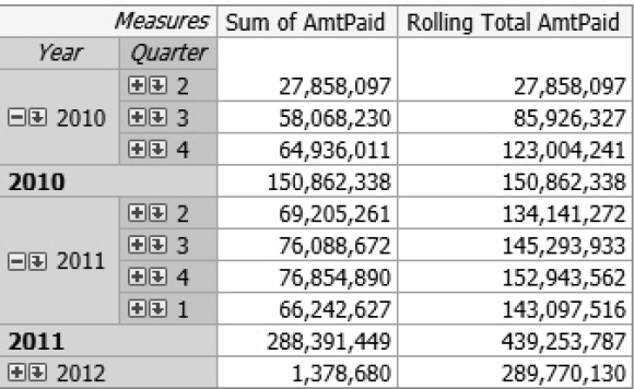
8. Verify the rolling totals in Figure 8.19, which are correctly computed both at the year and quarter level.
Figure 8.19: Rolling Totals in an OLAP Cube
8.3.3 Restricting Data Access with MDX
In this section, you build an MDX expression that enables a claims representative to view only claims he or she has processed. This expression is built and implemented in SAS OLAP Cube Studio.
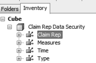
1. Navigate to the Claim Rep Data Security cube on the Inventory tab of SAS OLAP Cube Studio.
2. Right-click the Claim Rep dimension as shown in Figure 8.20. Select Properties. This is important because it attaches the security MDX expression to the dimension.
Figure 8.20: Claim Rep Data Security Cube
3. On the Authorization tab in the Claim Rep Properties dialog box, select SASUSERS, and click Edit Authorization.
Figure 8.21: Cube Dimension Properties
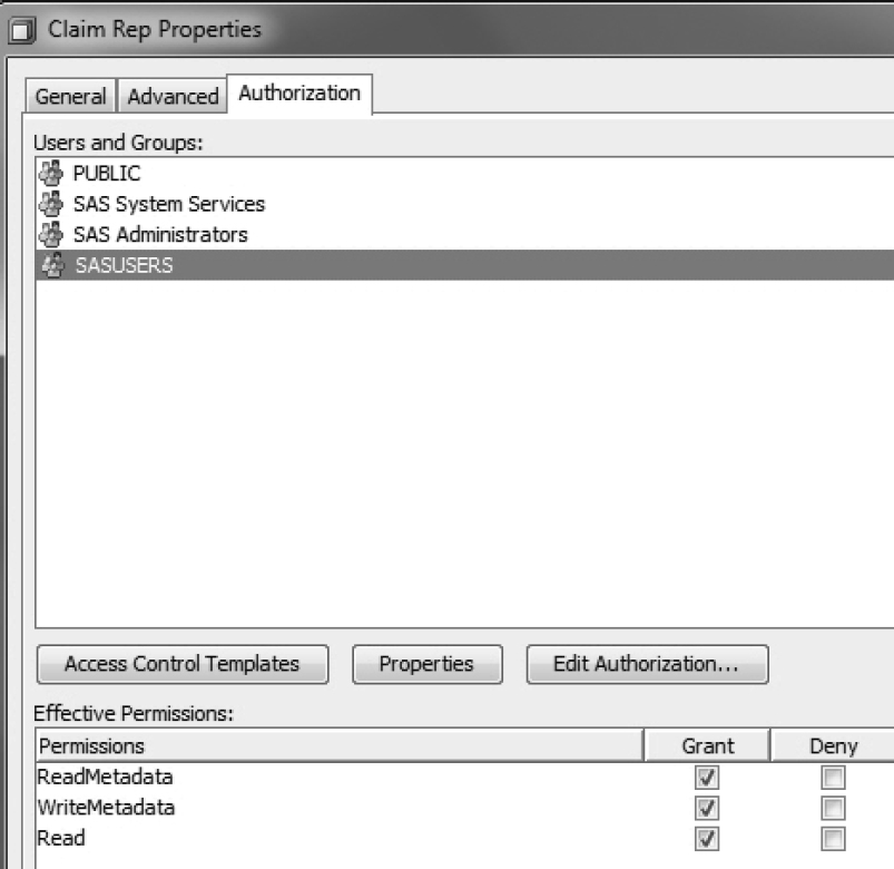
If you were using an industry application, it would create a security expression for a group of users. An example of this is the group containing claims representatives.
Edit Authorization is active only if the group has explicit Read permissions as shown in Figure 8.21.
4. Create the MDX expression.
Figure 8.22: Create Security Expression in SAS OLAP Cube Studio
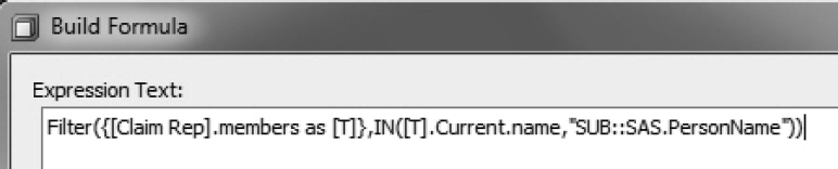
a. SUB:: can be considered a pseudo SAS format. It retrieves the value of SAS.PersonName. This value is substituted in the current value of Name from the ClaimRep dimension. If claims representative Jason logs on to view the cube, then his semi-resolved security expression is:
Filter({[Claim Rep].members as [T]}, IN(Jason))
b. The FILTER function takes two arguments. The first is the set of all members from the ClaimRep dimension. The second is the criteria for filtering.
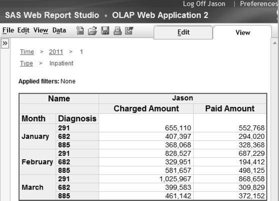
5. To demonstrate that the security expression works in SAS Web Report Studio, create an information map from the cube. Then, create a report in SAS Web Report Studio from the information map.
a. Log on as Jason to see that the report only returns his claims.
Figure 8.23: OLAP Security in SAS Web Report Studio
b. Log on as Renu and verify that the security expression works for her.
Figure 8.24: OLAP Security in SAS Web Report Studio

8.4 Computing Health-Care Metrics in an OLAP Cube
Healthy Living Inc. measures costs on a per member per month (PMPM) basis. Its analysts break down this metric by a number of slicer elements including unit of time, health plan, and type of health utilization. Although costs are additive across all slicer elements, member counts are not.
Table 8.6: Metrics Computation in the Health-Care Industry
| Month | Plan | Category | Member Count | Total Paid | Paid PMPM |
|---|---|---|---|---|---|
| 2010-05 | Bells and Whistles | ER | 1,477 | $ 1,272,462 | $862 |
| 2010-05 | Bells and Whistles | Inpatient | 1,477 | $ 4,129,499 | $2,796 |
| Incorrect Member Count | Bells and Whistles | All | 2,954 | $ 5,401 ,961 | $1,829 |
| Correct Total | All | 1,477 | $ 5,401 ,961 | $3,657 |
It is incorrect to add member counts across service categories. As a result, Paid PMPM is incorrect when it is derived from aggregating data at the service category level.
In this section, an OLAP solution is introduced that overcomes this data challenge. A cube is built from summary data sets containing accurate costs and member counts. The summary data sets enable the cube to correctly compute Paid PMPM metrics. The OLAP solution consists of three different steps.
1. Manipulate the Encounter and Demographics tables to create two additional tables.
2. Create three summary data sets with the tables from step 1.
3. Build a cube in SAS OLAP Cube Studio using the data sets created in step 2.
Many health-care companies have sophisticated data marts, so the first step might not be necessary in an industry application.
8.4.1 Data Manipulation
In this section, you create two tables. The first table, EncounterAgg, summarizes encounters by month, plan, and category. The second table, MemberMonths, summarizes enrollment by month and plan.
Because the Encounter table does not contain the member’s plan, combine the table with the Demographics table, which does contain the member’s plan.
proc sql;
create table Encounter as
select a.memberid,a.YearMonthDOS as Month, a.Category,b.Plan,
sum(AmtPaid) as PaidTot, count (distinct claimid) as Visits
from dw.Encounter a, dw.Demographics b
where a.memberid=b.memberid
group by a.memberid, a.YearMonthDOS, a.Category, b.Plan;
quit;
Summarize the Encounter table to aggregate costs across month of service, plan, and service category.
proc sql;
create table EncounterAgg as
select Month, Plan, Category, sum(PaidTot) as PaidTot,
sum(Visits) as VisitsTot
from Encounter
group by Month, Plan, Category;
quit;
Create the MemberMonths table, containing one row per member for every month of his or her enrollment. Expand the Demographics table to a member month level with the use of an OUTPUT statement embedded inside a DO loop.
data MemberMonths(keep=MemberID Plan Month MemberMonths);
set dw.demographics;
do Month=EffectiveDt to TermDt;
YearMonthDOS=Month;
MemberMonths=1;
output;
Month=intnx('Month',Month,1,'b')-1;
format Month yymmdd10.;
end;
run;
Aggregate the MemberMonths table with the following code:
proc sql;
create table MemberMonthAgg as
select Month,Plan,sum(MemberMonths) as MemberMonths
from MemberMonths
group by Month,Plan;
quit;
8.4.1 Summary Data Sets
This section combines the MemberMonthAgg table and the EncounterAgg table to create three summary data sets.
Program 8.1: Creating Summary Data Sets for the OLAP Cube
proc sql;
create table dw.MMAgg1 as
select b.Month, b.Plan, b.Category,
sum(a.MemberMonths) as MemberMonths,sum(b.PaidTot) as PaidTot,
sum(VisitsTot) as VisitsTot
from MemberMonthAgg a, EncounterAgg b
where a.Plan=b.Plan and a.Month=b.Month
group by b.Month, b.Plan, Category;
create table dw.MMAgg2 as
select Month, Plan, max(MemberMonths) as MemberMonths,
sum(PaidTot) as PaidTot, sum(VisitsTot) as VisitsTot
from dw.MMAgg1
group by Month, Plan;
create table dw.MMAgg3 as
select Month, sum(MemberMonths) as MemberMonths, sum(PaidTot) as PaidTot,
sum(VisitsTot) as VisitsTot
from dw.MMAgg2
group by Month;
quit;
Here are some key observations:
MMAGG1 is the most detailed data set, and MMAGG3 is the most summarized data set.
MMAGG2 computes member months using the MAX function, rather than the SUM function. This is important because member months cannot be aggregated across service types. The MAX function prevents any double-counting of member months.
MMAGG3 is derived from MMAGG2. As the MMAGG3 table aggregates across plans, member months are aggregated correctly using the SUM function.
Here are the three tables:
Table 8.7: MMAGG1 Table
| Month | Plan | Category | Member Count | Total Paid | Paid PMPM |
|---|---|---|---|---|---|
| 2010-05 | Bells and Whistles | ER | 1,477 | $ 1,272,462 | $862 |
| 2010-05 | Bells and Whistles | Inpatient | 1,477 | $ 4,129,499 | $2,796 |
Table 8.8: MMAGG2 Table
| Month | Plan | Member Count | Total Paid | Paid PMPM |
|---|---|---|---|---|
| 2010-05 | Bells and Whistles | 1,477 | $ 5,401 ,961 | $3,657 |
Table 8.9: MMAGG3 Table
| Month | Member Count | Total Paid | Paid PMPM |
|---|---|---|---|
| 2010-05 | 2,900 | $ 10,852 ,373 | $3,742 |
8.4.3 Creating an OLAP Cube from Summary Tables
In this section, you build a cube with the following characteristics.
• It is sourced from summary data sets.
• It specifies different ways of data aggregation.
• Because data aggregation is driven by summary tables, the cube contains only one dimension. This is a limitation of the approach.
• It includes formulas for metric computations.
1. On the Cube Designer - General page, select Fully summarized table as Input Type. This sources the cube from summary data sets.
2. In Cube Designer - Input, move MMAgg1 to Base table.
3. Create the Type dimension with Month, Plan, and Category levels.
A cube based on summary tables is limited to one dimension. As a result, it lacks the true slice-and-dice functionality that accompanies multiple dimensions. However, a careful design of the single dimension partially makes up for the loss of multiple dimensions.
In an industry implementation, the Type dimension should be as robust as possible, consisting of data elements from dimensions such as Plan, Time, Provider, Service Category, and Geography. The following dimensions and their associated data elements are good candidates for inclusion:
Plan: Type of Plan (Medicare or Medicaid or Private Insurance) and Plan Name
Time: Year, Quarter, and Month of Service
Provider: Provider Group (Hospital Chain or Clinic Group Name), Name of Provider (Hospital or Clinic)
Service Category: Billing Facility (Inpatient Hospital or Outpatient Hospital or Physician), Location of Services (Inpatient or Outpatient or ER or Physician’s office), Services Provided (DRG or Procedure Code)
Geography is determined by the U.S. Department of Commerce, Bureau of Census or by a priori by the health insurance company.
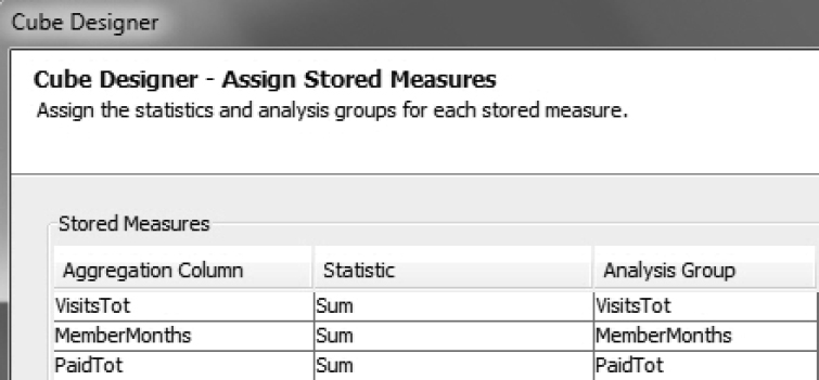
4. In Cube Designer - Select Stored Measures, move MemberMonths, PaidTot, and VisitsTot to Selected.
5. In Cube Designer - Assign Stored Measures, link measures to columns in summary tables using the Aggregation Column. It is important that columns have the same name across different summary tables.
Figure 8.25: Create Measures
6. In Cube Designer - Edit Measure Details, change measure formats or captions as needed.
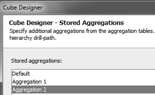
7. In Cube Designer - Aggregation Tables, move summary data sets MMAGG1, MMAGG2, and MMAGG3 to Selected tables.
8. In Cube Designer - Stored Aggregations, note that an aggregation named Default has already been created. This aggregation is created from MMAGG1, the cube’s base table. Click Add to create additional aggregations.
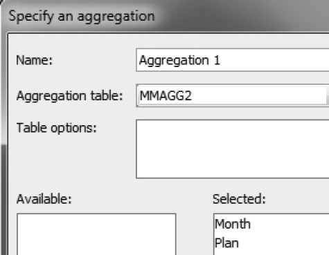
9. Create additional aggregations, specifying the correct source table.
a. Create Aggregation 1 at the Month and Plan level, and source it from MMAGG2.
Figure 8.26: Creating Custom Aggregations
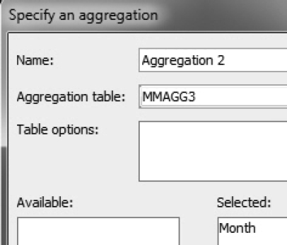
b. Create Aggregation 2 at the Month level, and source it from MMAGG3.
Figure 8.27: Creating Custom Aggregations
c. Confirm these aggregations in Cube Designer - Stored Aggregations.
Figure 8.28: Custom Aggregations in OLAP Cube
10. Create a cube.
11. Add formulas for metrics computation.
a. Select Actions → Calculated Members.
b. Select Simple Calculations.
c. Enter a formula for Paid PMPM. This is a ratio of PaidTot to MemberMonths.
d. Repeat steps a through c for additional metrics, such as Visits PMPM.
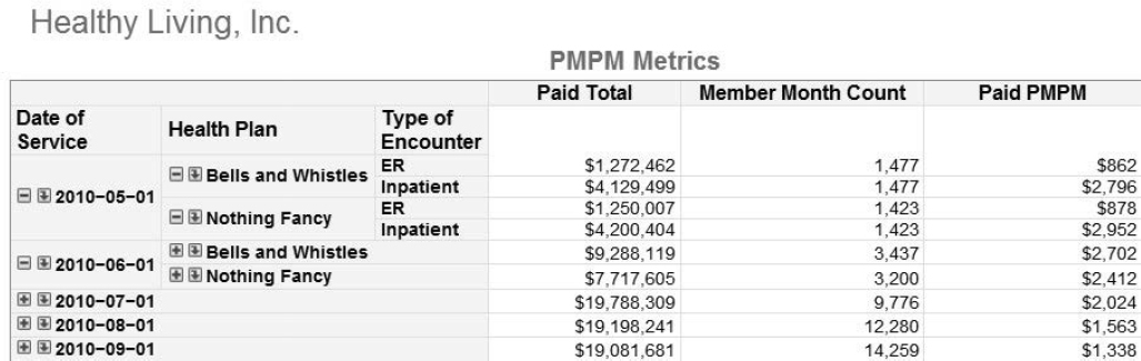
12. Verify that the cube correctly computes Paid PMPM.
a. Create an information map from the cube. Create a report in SAS Web Report Studio from the information map.
b. Verify that the cube correctly computes Paid PMPM.
Figure 8.29: PMPM Metrics
8.5 Conclusion
In this chapter, you built three OLAP solutions for the health-care industry.
In the first OLAP application, you created a powerful and wide-reaching analytical solution from a single data source. You built a cube from a star schema database, incorporating many facets of health-care data. You leveraged prompted filters in an information map to source multiple reports.
In addition to sourcing SAS Web Report Studio reports, the cube and the subsequent information map serve as independent analytical tools. In SAS Enterprise Guide, SAS programmers can use them to conduct ad hoc analysis, avoiding time-consuming data pulls from multiple database tables. Business analysts can use SAS Add-In for Microsoft Office to manipulate and analyze the cube in Excel.
In the second OLAP application, you implemented security for OLAP data via MDX. MDX is a powerful, but difficult, language. Learning MDX became less challenging by leveraging the point-and-click interface in SAS Enterprise Guide to extract MDX expressions.
In the third OLAP application, you addressed a data aggregation challenge unique to the health-care industry. In health-care data, member counts–the basis of metric computations–are not always additive. The OLAP solution that you built relied on multiple summary data sets with correct member counts. In an industry implementation, the number of summary data sets can quickly become unmanageable. However, the SAS Macro Language provides an excellent way to generate and maintain summary data sets.
8.6 Note
1. This solution was first presented in a paper by John Leveille of d-Wise Technologies, Inc. See Leveille, John. 2011. “Healthcare Intelligence: The Challenge of OLAP for Healthcare Data.” Proceedings of the SAS Global Forum 2011 Conference. Cary, NC. SAS Institute Inc. Available at http://support.sas.com/resources/papers/proceedings11/TOC.html.