The time series data of the customers was aggregated to one single row per customer ID. Some of the business questions raised needed the exclusion of some variables that could possibly explain the client behavior through their life cycle. The variables that were identified for analysis were the following:

• Customer ID: This was used as an ID variable and not for analysis.
• Tenure: The number of years the customer has been with the brokerage firm. Right censoring was done in 31 instances where the customer is still active after being with the firm for 20 years.
• AUM: Assets under £0.5 million are classed as 1, between £0.5 and £1 million as 2, 2 to £5 million as 3, and above £5 million as 4.
• Risk appetite: As part of its compliance process and to better understand the customer's investment needs, the brokerage had assigned a low risk (1), medium risk (2), and a high risk (3) strategy value to the customer's risk appetite.
• Fund performance: At the end of the day, the customers were interested in growing their capital invested via the brokerage.
• Investment potential: This is the level of investment that the client can have. The client may have already invested this money elsewhere. The fund manager was interested in the investment potential that the brokerage customers offered and this was one of the reasons for the takeover. It had a value 1 (£1 – £5 m), 2 (£5 – £10 m), and 3 (£10 million+).
• Investment involvement: This is a variable that is linked to compliance requirements mandated by certain oversight bodies, such as the Financial Conduct Authority (FCA) in the UK. Clients have varying levels of preference regarding how much time they want to spend actively managing their investments. Also, not all clients have prior investment experience and their level of understanding of the financial instruments available may be limited. In such cases, the brokerage firm has a responsibility to either offer advice or ensure that the client has sought advice independently prior to investing. The variable is classed as 1, 2, and 3 for clients with low, medium, and high involvement, respectively.
• Complex product: This is classed as 1 if the customer holds complex products and 0 in other cases. Some of the complex products may involve higher investment criteria, may require more understanding of how they are structured, or might be customized offerings.
• Complaints: Unfortunately, like any business, the brokerage firm had received complaints in the past. The fund managers were busy trying to understand the nature of these complaints and resolve them. Instances where clients had complained have the value 1.
• Region: All these customers were UK based and the values represented the geographic location where they were primarily based.
• Censor: Right censoring was done in the instances where clients were still active.

PROC UNIVARIATE and PROC CORR were run to get a better understanding of the dataset, survival_analysis.

This was PROC UNIVARIATE normal distribution code:

PROC UNIVARIATE Data = survival_analysis Normal Plot; 
   Var tenure; 
   Cdfplot tenure; 
RUN; 

The UNIVARIATE procedure has output four statistical tests to check the assumption that the data is normally distributed. The Shapiro-Wilk, Kolmogorov-Smirnov, Cramer-von Mises, and Anderson-Darling tests are produced as part of the tests for normality. The Shapiro-Wilk test is relevant in this case as the sample size is less than 2,000. The test rejects the hypothesis that the data is normally distributed:

In Figure 6.4, the extreme observations highlight the fact that some of the clients have left the brokerage within the first year. Whereas, there are instances when some of the clients have left the brokerages in the past year after having been a customer for 20 years. The recent departures after a long stay may potentially be linked to the takeover of the brokerage by the fund manager.

This was an aspect that needed to be looked in to. Without analyzing further, the analyst wasn't keen to remove or transform any extreme observations from the study:

The preceding diagram highlights the fact that the mean and median values are quite close. The quantiles plot highlights that the tenure is fairly distributed across the quantiles line. Ideally, the skewness should be close to 0. The skewness for tenure is 0.33092243 in our case. The kurtosis should ideally be close to 3 but it is - 1.0416142. The negative kurtosis highlights a lighter tail and is also known as platykurtic distribution:

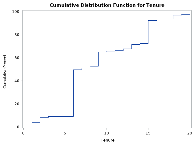
We also requested for a cumulative distribution (cdf) plot for tenure. The chart plotted includes both censored and non-censored data. Let's look at the cdf plot for the uncensored data:

The PROC UNIVARIATE normal distribution code for uncensored is as follows:

PROC UNIVARIATE Data = survival_analysis (where=(censor=0)); 
   Var tenure; 
   Cdfplot tenure; 
RUN; 

The CDF plots in Figure 6.4 and Figure 6.5 are different as the population in the latter is a subset and only includes the uncensored data. The uncensored data has already experienced the event of churn. The CDF plot highlights the chances of a client churning. The biggest increase in churn is happening at the 6^th, 9^th, and 15^th anniversaries of the clients:

The following is the correlation analysis:

PROC CORR Data = survival_analysis; 
   Var Risk_appetite Fund_performance Inv_potential Inv_involvement AUM Complex_prod Complaints; 
RUN; 

All variables have a low correlation with other variables. None of the variables have a correlation value of more than 0.4: