When Prof Cox got the data, she realized that it contained details of both past and current customers. She decided to get rid of the past customers. Vogue shouldn't be so keen on spending their energy on seeing how segments have evolved over time. She remembered her early days at the company, where the simple mantra was to get almost any client no matter what their profile was. As long as they had money to invest and passed the regulatory requirement checks, Vogue was more than happy to take them on board. Yes, the trio might be interested in seeing the segmentation comparison over time, but then their immediate task as she understood it was to present the current profiling to the board and their team to draw up a marketing strategy. She ran some descriptive statistics on the data and she found that there were a few outliers. These outliers were clients with extremely high and low AUM values, which, after a few checks with the data governance team, she found were historical test case entries in the system. She made a point of removing these entries. She didn't want such outliers to heavily influence clustering. There would have been a chance that such a customer would not fit in most of the clusters and they might end up in a single cluster representing extreme values. Far worse was the scenario that they would be so different from the rest of the customers and from other outliers that the output may have a lot of clusters with individual records.

She also noticed that some of the data rows contained information about secondary customers. Even where it seemed to be a joint account, Vogue had put in a flag to say which of them was a primary customer. She was only keen on the primary customers as these were the people that Vogue had initially approached while they were prospects, or these were the people that they now interacted with to manage their affairs. None of these primary customers, according to the data governance policy of the company, were guardians or legal representatives of the account holder.

Vogue had not opened up its entire customer database in terms of sharing each and every detail they held about customers and their transactions. The variables that were shared were:

1. Gender
2. Age
3. Education
4. Occupation
5. Customer tenure
6. Country of citizenship
7. Country of birth

8. Risk appetite
9. Investment involvement
10. Complex product held
11. Investment potential
12. AUM
13. Net worth of secondary
14. Fund performance

With all these variables, there was a chance that some of them may be correlated. Correlated variables could heavily bias the cluster structures. Also, in many business scenarios, the number of variables available at the initial modeling stage far exceed the required or the manageable number of variables. The foremost criteria in variable selection should always be relevance to business goals. However, in segmenting credit card customers, let's assume that you have demographic, psychographic, and transactional-level details of customers' credit cards and their product relationship with various other bank departments. The total count of such variables could end up being in the hundreds in a typical data warehouse. Aren't all these three broad categories-demographic, psychographic, and transactional data-relevant? Yes, they are. However, some of the information could be of little additional value, as multiple variables could be pointing to the same conclusion. Variables such as a high credit rating, settled loan accounts, high disposable income, a large savings balance, and an occupation as a doctor may all point to the fact that the customer has a high probability of repaying all of the borrowed money. So, do we need all these variables? Think in terms of hundreds of such variables in a dataset. Shouldn't we save some of our computational resources and modeling time, and have a smaller list of variables to model? Should we be collecting so many data variables and putting effort into maintaining them in a database if they all point to the same factor? Clustering for large datasets requires high computational resources and hence it's best to reduce redundant variables. If the dataset is being specifically maintained for segmentation, then by using fewer variables we can also optimize data collection and storage. Even though 14 variables were shared for analysis, only 7 were considered fit to be considered for modeling. The reason for reducing the number of variables was a mix of data quality and a reluctance to accept insights that were generated using all variables. The final variables selected for analysis are mentioned in the varclus procedure in the following paragraph.

One of the ways to reduce the number of variables used is by running Proc varclus and looking at the cluster structure. Proc varclus is usually used in initial model building, and this is followed by running some other clustering procedures to get the final segmentation model. Let's run the varclus procedure for Vogue's dataset. The number of variables is just seven, and not the hundreds that a modeler could be faced with. It would be worthwhile to see whether varclus still adds value.

Here is an example of clustering via Proc varclus:

Proc varclus data=cluster_model; 
var age aum risk_appetite fund_performance investment_potential      investment_involvement complex_product; 
run;

After varclus execution, we can see that all the variables are initially put in a single cluster:

The clustering continues, and now we have a two-cluster solution with further details about the clusters:

Proc varclus starts by assuming that all observations are in one cluster. It continues to split the observations until the second eigenvalue is greater than one. In our case, the clustering process stops after the creation of the second cluster. In the cluster summary for two clusters in Figure 7.11, we can see that we are left with two clusters. The first cluster contains five variables and the second cluster two variables. The total variation of 3.68 explained by the solution of two clusters is higher than the total variation of 2.7, which is explained in the one-cluster solution.

In the preceding table with the R squared values, if the variable has a low R square with its nearest cluster, the clusters are expected to be well separated. The last column contains the (1-R²_own)/(1-R²_nearest) for each variable. Small values of the ratio indicate good clustering. However, the AUM variable in particular has a high value. In the Standardized Scoring Coefficients table, each variable is assigned to one cluster only, hence each row has only one non-zero value. The values can be both positive and negative:

In Figure 7.12, we can see the structure of the cluster, the inter-cluster correlations, and the history of the clustering solution. The inter-cluster correlation in our business problem is quite low. The model says no cluster meets the criterion for splitting. As discussed earlier, this is due to the second eigenvalue being less than one after the creation of the second cluster:

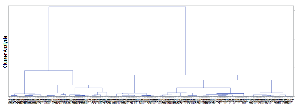
In Figure 7.13, we can see the cluster structure. The varclus procedure has performed a clustering oblique multiple-group component analysis. The cluster procedure, however, performs the hierarchical clustering of observations. Proc varclus, as discussed, is used primarily for variable reduction as it works well with variables that are correlated. Could both these methods produce different clustering solutions to our business problem? Let's try running a cluster procedure and see the differences. We will use the ward method as part of the procedure.

Here is clustering via Proc cluster:

Proc cluster data=cluster_model method=ward ccc pseudo out=tree plots(MAXPOINTS=300); 
   id custid; 
   var age aum risk_appetite fund_performance investment_potential investment_involvement   complex_product; 
run; 

In applying the cluster procedure, we have used the ward method. Most clustering methods are focused on distance metrics or measures of associations. The ward method instead tries to look at the clustering problem from an analysis of a variance problem. It starts with n number of clusters with each having size 1. It then aggregates and starts forming larger clusters with a higher number of constituents, and keeps on aggregating until reaching the stage of one large cluster containing all the observations. We have used the max points option in the code due to the high number of clusters being produced. If you look at the covariance matrix in Figure 7.14, you can see that, just like in the varclus procedure, the second eigenvalue is less than one. After this point, the eigenvalue continues to decline. The proportion of variance explained up to this point is 60.41%:

The cluster history table gives us the cubic clustering criterion. At clusters 3 and 4, this goes into negative territory, thereby indicating the presence of potential outliers. Values between 0 and 2 tend to indicate potential clusters. Values greater than 2 or 3 generally indicate good clusters. At cluster 2, we have a value of 1.24. Remember, varclus suggested a two-cluster solution:

Let's look at the CCC graph in Figure 7.15. The graph shows a peak at cluster 2 and then the next at cluster 7. This correlates with the partial cluster history shown in Figure 7.14. While evaluating the CCC graph, we are on the lookout for spikes of positive values to determine the ideal cluster solution.

We also have the option of using the Pseudo F and the Pseudo T-Squared graphs in Figure 7.15. Relatively large values of Pseudo F are indicative of good clusters. This value is the highest at the start of the graph and the value of 136 is the highest, as also observed in Figure 7.14. To use Pseudo T-Squared, one should look at sudden and large decreases in value. Clearly, the steepest decrease in value is at cluster 2, with fairly large decreases at clusters 5 and 7 too.

One point that analysts should note is that while using Proc cluster, it is quite common for the code to produce the following message: WARNING: Ties for minimum distance between clusters have been detected at n level(s) in the cluster history. This happens as discrete data isn't usually as smooth as the textbook example data used. This warning can be ignored. However, there are ways in which the ties can be further explored and one solution is to club a few variables together to reduce the presence of ties. However, we shall not delve into this issue and will ignore the T values in the last column in Figure 7.14:

We have reached the stage where both the varclus and cluster procedures are suggesting a two-cluster solution. However, does this meet the business objectives? Is clustering or modeling independent of feedback from the business? Will the hedge fund benefit by having a two-cluster solution?

In any business, a two-factor solution may be perceived as being a sort of binary outcome. Maybe all the good customers are in one cluster and all the bad or undesirable customers, or customer traits, are in the other cluster. This is an overly simplistic solution for most businesses. When Prof Cox looked at the two-cluster solution from an implementation perspective, she wasn't too happy. Clusters 3 and 4 don't make sense either, as they have a negative CCC. The Pseudo T-Squared suggests potentially good clusters at the 5 or 7 level. She felt that having seven clusters might be a bit too much for the business, as they will potentially have to deal with the fallout of having seven segments to deal with in terms of customized strategies. A cluster solution of five looked good to her from the statistical metric support and business implementation perspectives.

A modeler may face this sort of situation in a practical scenario rather than a textbook case. A textbook case will always pitch for a two-factor solution. But is the solution always so simple? Clustering at some level is a business decision that isn't based on a purely statistical basis. The overall aim of segmentation should be to find clusters of customers that have a statistical rationale, but also to segment the customers into a manageable number of clusters that help produce effective strategies. Prof Cox decided to go for the five-cluster solution and see what impact it had on the segments generated.

Unfortunately, the SAS University Edition on which the modeling has been done for the book doesn't support some visual features that help to effectively showcase the output of Proc tree. However, the full edition of SAS software produces a more visually appealing chart of the procedure. For our current consumption, only the tabular output has been shared in Figure 7.17. The procedure is going to help us to assign the cluster number to each of our customer IDs. This is an important step, as after this we can go ahead and try to understand the profiling of our cluster constituents.

This is a Proc tree five-cluster specification:

Proc tree data = tree out = cluster_output nclusters=5; 
   Id custid; 
   Copy age aum risk_appetite fund_performance investment_potential 
      investment_involvement complex_product; 
Run; 
 
proc print data=cluster_output(drop=clusname); 
run; 

Although there was a fair bit of confidence in going with the model generated up to now, there were a lot of other alternate models considered in the build phase. The models differed in the type of clustering used, the data standardization used, and the mix of variables used to build the models. Let's produce an alternative model using the following code:

/*Age and AUM have been dropped in the model*/ 
Proc varclus data=cluster_model; 
   Var risk_appetite fund_performance investment_potential         investment_involvement   complex_product; 
run; 

The output in Figure 7.18 shows that the model did not produce any splitting and suggested a single-cluster solution. This happened after two key variables were dropped from the modeling solution:

The chart reconfirms that we are left with a single cluster solution after the omission of two variables from the alternate model code:

Prof Cox gave the five clusters a name and recommended a strategic direction for Vogue to take regarding the clusters. As a modeler, the business expects that the model built is statistically robust. It can be validated and is documented with a high degree of governance during the build, approval, and implementation phases. However, modelers at times tend to forget how simple summaries of the model can help to create a greater understanding of the model and help trust the insights generated. The next few pages are dedicated to showcasing how Prof. Cox summarized the output from the model:

She further described the segments in Figure 7.19 as:

• Star performers: These customers are the ideal age group. Probably the happiest Vogue customers in terms of returns on investment. They have a high level of AUM and there is a potential for further investment. They are medium risk takers and have no preference regarding simple or complex products. They are the smallest cluster of the five.
• Cash cows: They are split across the age groups. They behave like cash cows for Vogue as they have low-to-medium AUM, yet are large in number and help to sustain the business. They are involved in their decisions and aren't risk takers. 76% of them have experienced low returns with Vogue. However, due to their low risk-taking preferences, and in general, lack of inertia to move to competitors, they are thought to be good for the business in the long run. 18% of them have experienced medium returns and this percentage could be further increased in the years to come.
• Nurture: They are split across age the groups and have a medium-to-high-potential to invest. They have experienced a mixed level of fund performance. Their risk appetite is quite high and they don't tend to have complex products. The most promising feature of this segment is that they have low-to-mid-level AUM. Given their potential to invest, with a bit more focus this segment could become a more exciting segment for Vogue. After all, this is their second biggest segment.
• Keen but not there: A fairly big cluster of younger individuals with lower involvement, low fund performance, low potential to invest, and low-to-mid-AUM. These are high risk takers who tend to have complex products. They could also benefit from being nurtured, but they are probably not mature enough from a prospective client perspective. This is a segment that Vogue should continue to watch out for and be patient with.
• Going nowhere: This segment has young members. They have low involvement in investing and lower potential. The lower potential might stem from the fact that they already tend to have high AUM with Vogue. However, the predominantly low fund performance that they might be facing could be a factor in them expressing lower investment potential. Vogue needs to look at this segment and see if relationship managers need to focus less on these customers.

So, how did Prof Cox define and describe the segments? The output dataset produced as part of the proc tree code in Figure 7.17 is where the cluster name is stored against each customer. However, the cluster name is a number and isn't a descriptive field describing the characteristics of the cluster/segment. Prof Cox had to produce some profiling tables from the output dataset. Let's look at them:

Age

AUM

Risk appetite

Fund performance

Investment potential

Investment involvement

Complex Product

Cluster summary

Cluster summary continued:

As you can see in Figure 7.20, we need to develop some profiling tables to understand the characteristics of our segment constituents. We can already see that the clusters differ between the mix of age groups, assets under management, and risk appetite. By adding profiling info using other variables for clustering, we can come up with descriptions of the segments. What Prof Cox has done is to go a step beyond and name the segments. Naming the segments is an easy way to remember the key characteristics of the segments. Some businesses prefer to name segments in a way that explains what each segment means to their strategy. There is no specific scientific way to describe and name a segment. The insights from profiling should make business sense, and the naming of segments should lead to the achievement of some business goals. Having named her segments and being ready with her proposed strategy for the segments, Prof Cox looked forward to sharing the modeling results with Vogue.