To explore the basic concepts of ARIMA, please refer to Chapter 2, Forecasting Stock Prices and Portfolio Decisions Using Time Series. In this section, we will try and find the best suited ARIMA model to our three series: classic, premium, and platinum account types. We will be using historic time series data (Figure 4.3) to generate forecasts for five periods.

This is the data setup and ARIMA identification for the classic account:

Data Past; 
input Cl Pr Pl; 
datalines; 
30.68 5.73 1.51 
30.65 5.74 1.53 
30.83 5.43 1.66 
30.9 5.3 1.72 
31.1 4.7 2.12 
31.05 4.73 2.14 
31.01 4.81 2.1 
30.7 5.01 2.21 
30.3 5.3 2.32 
29.3 6.4 2.22 
29.3 6.5 2.12 
28.8 7.3 1.82 
28.8 8.1 1.02 
28.7 8.3 0.92 
28.6 8.34 0.98 
28.4 8.37 1.15 
27.6 9.01 1.31 
26.5 9.5 1.92 
26 9.8 2.12 
25.3 10.3 2.32 
; 
Run; 
 
Ods Graphics On; 
PROC ARIMA Data=Past; 
identify var=Cl scan esacf; 
RUN; 
 

The first step in the ARIMA model is to identify the autoregressive (AR) – p, differencing – d, and moving average (MA) – q components of the model. We have used the scan and the esacf options, which will help us in identifying the values of p, d, and q.

The chi-square probability values for the scan option in Figure 4.9 show that 0.701 (AR2, MA0) and 0.0671 (AR0, MA2) are the first instances when at a five percent level of significance we failed to reject the hypothesis of no correlation:

Let us also look at the chi-square test for the esacf option. It shows that the first instance where at a 5 percent level of significance we failed to reject the hypothesis of no correlation is 0.2419 (AR1, MA0) and 0.0598 (AR0, MA1). We have other values of p and q also suggested by the esacf option. For the classic account customers, we have seven model choices: ARMA (2,0), ARMA (0,2), ARIMA (1,1,0), and ARIMA (0,2,0) based on scan output, and ARMA (1,0), ARIMA (0,1,0) or ARMA (0,1) based on esacf output:

Figure 4.10 contains some of the plots of classic account customers without any model estimation. There is a gradual decline in the ACF plot, indicating a stationary time series. It may be a better idea to use at least one of the differencing models to compare the available options for modeling the classic account customers via the ARIMA methodology.

Here is the code for estimating models for classic account customers:

PROC ARIMA Data=Past; 
identify var=Cl(1); 
estimate p=1; 
forecast lead=5 interval=semiyear out=Cl1; 
identify var=Cl; 
estimate p=2; 
forecast lead=5 interval=semiyear out=Cl2; 
identify var=Cl; 
estimate q=1; 
forecast lead=5 interval=semiyear out=Cl3; 
RUN; 

In Figure 4.11, the first drawback of the ARIMA (1,1,0) model is that although the t value of autoregressive parameter AR1,1 shows that the term is significant, the p value indicates that at a 0.05 level, the term is insignificant. As soon as we move to the autocorrelation check of residuals, we encounter another problem. This section of the output relates to the white noise test. The null hypothesis is that no autocorrelations of the series are significantly different from 0 for the given lags.

Remember that ARIMA is based on autocorrelations being present. Given the p values >0.05 we cannot reject the null hypothesis. This means that autocorrelations are present for none of the lags. There is no need for an ARIMA model when we have used p=1, d=1, and q=0.

In Figure 4.12, let's evaluate our next model, ARMA (2,0). The term AR1,1 is significant. The term AR (1,) is insignificant and doesn't add any value to the model, as shown in the following table:

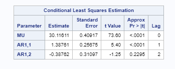
In this model too, we have an issue with the white noise null hypothesis. Since it cannot be rejected at the given p values, we should ideally discard this model and look for another alternative. See the following tables:

In Figure 4.13, we have the output of the ARMA (0,1) model. A quick check shows that we can reject the null hypothesis at all the default lags that have been tested. This shows the need for an ARIMA model. The t value and the p statistic indicate that the term MA1,1 is significant. Usually, we should go with a lower AIC and BIC model. In both Figure 4.11 and Figure 4.12, we have a lower AIC and BIC. However, due to the inability to reject the white noise null hypothesis, it would be prudent to go with the higher AIC and BIC in ARMA (0,1). A lower AIC and BIC would be preferable when comparing models, but due to the inability to reject the white noise null hypothesis, we are going ahead with the relatively higher AIC and BIC. Remember, we have six potential models for the classic account types that we can test. We aren't going to test for all of them and will now continue to look at some more diagnostics of the classic account series ARMA (0,1) model. See the following table:

When comparing the ACF plot in Figure 4.10 and Figure 4.14, you can observe that ACF decreases significantly more in the latter figure where we have plotted the ARMA (0,1) model. However, there still seems to be some stationarity and the ACF plot doesn't show sudden declines till Lag 3 in Figure 4.14:

On examination of the residual normality diagnostics in Figure 4.15, it seems that the residuals are normally distributed. We can go ahead and have a look at the forecasts:

In Figure 4.16, we have the forecasts for classic customer account types for five periods. We will compare the ARIMA forecasts with Markov model output once we have generated output for the premium and platinum customer accounts:

This is the ARIMA identification code for premium and account:

Ods Graphics On; 
PROC ARIMA Data=Past; 
identify var=Pr scan esacf; 
identify var=Pl scan esacf; 
RUN; 

From the chi-square probability values from the scan option, p+d =2 and q = 0 seems to be a fair model option given that the first value in the matrix greater than 0.05 in Figure 4.17 is AR2 MA0:

For the esacf option, AR1 MA0 and AR0 MA2 fit the criterion of first value greater than 0.05. We already have AR1 MA0 and hence AR3 MA0 doesn't look like an attractive option, unless of course higher-order differencing is needed to achieve a stationary time series. Let's fit an ARIMA (1,1,0), ARMA (1,0), and ARMA (0,2) model and select the best possible option for forecasting premium account customer counts:

Here is the code for estimating models for premium account customers:

PROC ARIMA Data=Past; 
identify var=Pr(1); 
estimate p=1; 
forecast lead=5 interval=semiyear out=Pr1; 
identify var=Pr; 
estimate p=1; 
forecast lead=5 interval=semiyear out=Pr2; 
identify var=Pr; 
estimate q=2; 
forecast lead=5 interval=semiyear out=Pr3; 
RUN; 

In Figure 4.18, the first drawback of the ARIMA (1,1,0) model is that although the t value of autoregressive parameter AR1,1 shows that the term is significant, the p value indicates that at a 0.05 level, the term is insignificant. As soon as we move to the autocorrelation check of residuals, we encounter another problem. This section of the output relates to the white noise test. The null hypothesis is that no autocorrelations of the series are significantly different from 0 for the given lags. Remember that ARIMA is based on autocorrelations being present. Given the p values >0.05, we cannot reject the null hypothesis. This means that autocorrelations are present for none of the lags. There is no need for an ARIMA model when we have use p=1, d=1, and q=0.

This is exactly the same result we got when we used a similar model to test the robustness of the model on the classic account series:

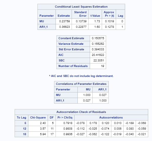
In Figure 4.19, let's evaluate our next model, ARMA (1,0). The term AR1,1 is significant. Compared to the model in Figure 4.18, we do not have an issue with the white noise null hypothesis. Since it can be rejected at the given p values, we can proceed to assess the model:

In Figure 4.19, let's evaluate our next model ARMA (1,0). The term AR1,1 is significant. Compared to the model in Figure 4.18, we do not have an issue with the white noise null hypothesis. Since it can be rejected at the given p values, we can proceed to assess the model.

The model in Figure 4.20 is also fitting well and has the white noise diagnostic test, and also has a significant t value. However, the model in Figure 4.19, which is the ARMA (1,0) model, has lower AIC and BIC values. Hence, this model will be suitable for forecasting the premium account series:

Figure 4.21 contains the forecasts for premium account customers based on the ARMA (1,0) model:

For the platinum account customers, let's try a slightly different approach to test the various models that fit the distribution. We will pick up the top recommendation from the scan and esacf table:

This is the ARIMA identification for the platinum account:

PROC ARIMA Data=Past; 
identify var=Pl scan esacf; 
RUN; 
 

Since we have decided to pick the top recommendation, let's use the first recommendation from the tentative order selection tests in Figure 4.22:

Here is the code for estimating models for platinum account customers:

PROC ARIMA Data=Past; 
identify var=Pl; 
estimate q=3; 
forecast lead=5 interval=semiyear out=Pl1; 
identify var=Pl; 
estimate q=1; 
forecast lead=5 interval=semiyear out=Pl2; 
RUN; 

Now have a look at the following tables:

For the ARMA (0,3) model, the t value is insignificant in Figure 4.23 for the MA1,3 model, whereas the t value is significant for the MA1,1 and MA1,2 models. The white noise test can't be rejected for any. However, for the ARMA (0,1) model in Figure 4.24, we see that the t value is significant and the white noise test can also be rejected:

Let's combine the forecasts of the Markov model and ARIMA, and compare them:

In the premium account forecast in Figure 4.26, the three model forecasts are close to the actuals:

For the classic and the platinum accounts, the forecasts from the selected ARMA models in Figure 4.25 and Figure 4.27 seem to deviate significantly from the trend of the historical data:

The finance team now has the option of choosing the forecast they want from any of the three models: the main forecasts from the observed transition matrix, forecasts from the alternate transition matrix based on marketing team inputs, and the forecasts from ARIMA models.