The stock price information was readily available from multiple sources. The modeler stored the stock price over the last couple of years. This information was collected on a daily basis. While getting the historical price movement wasn't a challenge, assessing which predictor variables could be important for the model was definitely intriguing. The modeler decided to use a bunch of financial ratios, econometric variables, and competitor-related information to build the model.

Financial ratios were important, as Mr. Jefferson wanted to test the significance of ratios used in the industry to predict the share price. A portfolio manager should always assess these sorts of ratios. The manager may decide to place a varying level of weight while investing, but these ratios are hard to ignore. The econometric variables, according to the modeler, were important, as there are a lot of economic factors that may be driving the share price. The competitor-related information is important, as the manufacturer of interest is one of many in a crowded mobile market. The fates of the manufacturers are interlinked. Product launches happen frequently, and customers switch loyalties at times, depending on the features and pricing of the products.

Let's take a look at the variables selected for modeling:

• Financial ratios and information:
  • Earnings per share (EPS): This is the earnings per outstanding shares of common equity of a company. It is one of the most important indicators of a company's performance. This ratio informs on the value that is available to stockholders. The higher the EPS, the more attractive it is for investors.
  • Price (PE) ratio: This is related to the EPS, as it is used as the denominator when calculating the PE ratio. A high PE ratio may be considered to be an average level for stocks of a different industry. However, given the stocks of two similar companies, the company with the lower PE ratio might be more attractive to the investor, as the upside potential of the stock price may be higher.
  • M1 money supply: This is the money supply of a country that is monitored by the central banks. The modeler, in this instance, created an index of the M1 money supply of the top 10 economies in the world.
• Econometric variables:
  • Gross Domestic Product (GDP) of selected economies: The modeler has created an index of the GDP of the top 10 economies in the world.
  • Inflation of selected countries: The modeler has created an index of the inflation of the top 10 economies in the world.
• Competitor and market related:
  • Global market share: This is the percentage of the global market share that the mobile manufacturer in question has.
  • Competitor basket index: This is an index of the growth of stock prices of major mobile manufacturing competitors.
  • Media analytics index: All of the news stories from major publications, opinions, and social media chatter are aggregated by certain media companies and given a score. The score represents how favorably the company is being perceived. The modeler wanted to include this as a probable significant predictor, as the product launches are debated intensively in the mainstream and social media.

The transformation that was done by the modeler was primarily to create various indexes. The indexes show the changes in value or percentage across various time periods. The base value of the indexes has been kept as 100 (or 100%). Any decrease in the value pushes the index below 100, and any increase keeps it above the base level. Different indexes used by the modeler are updated at various time intervals. The media analytics index is updated monthly, the GDP index quarterly, and the global market share on a six-monthly basis.

The predictor variables were sourced by the modeler from various sources, and underwent some sort of transformation or data cleaning. The stock price data didn't undergo any transformation. The modeler decided to do a data check prior to modeling. He ran the PROC UNIVARIATE code and produced the following output:

PROC UNIVARIATE code:

PROC UNIVARIATE DATA=raw; 
ID date; 
VAR stock; 
RUN; 

The PROC UNIVARIATE partial output was as follows:

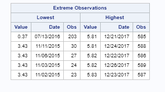
To understand the computation of the basic statistical measures, the modeler turned his attention to the output box of the extreme observations. These observations had the biggest hand in the variance that was captured by the statistical measures. He noticed that the value 0.37 of stock stood out as being quite low, given that the mean, median, and mode of the variable were all above 4:

He wanted to understand the impact that this observation had on the normal distribution plot of the variable. He ran the following code to generate the normal distribution plot.

The PROC UNIVARIATE normal distribution code is as follows:

PROC UNIVARIATE DATA=raw; 
HISTOGRAM Stock / normal(percents=20 40 60 80 midpercents) 
                     name='MyPlot'; 
INSET n normal(ksdpval) / pos = ne format = 6.3; 
RUN; 
 

The output is as follows:

The normal distribution is just one of many distributions used to describe the spread of the data. The normal distribution is among the most widely used distributions, and is also called a bell curve. It plots the probability distribution of stock, in this case. Most of the values of stock are expected to be around the mean, and the variables are expected to be equally distributed around the center. A normal distribution is defined by its mean and standard deviation. A standard normal curve has a mean µ = 0, and standard deviation σ = 1. If the dataset is normal distributed, then 68% of all observations are within σ = 1, and 95% of them fall within σ = 2.

In the case of the stock, the modeler noticed a couple of things. Towards the mean, most distributions have a value of around 4.5 or 5.5 U.S. dollars. He also noticed that there seems to be a particular data point with a very high standard deviation that is falling outside the bell curve, and is located towards the left side of the distribution. Upon further investigation, the modeler realized that there is a stock value of 0.37 on July 13, 2016. This was an error in the creation of the SAS dataset, and, in fact, the value of stock observed on July 13, 2016, was 4.37. After correcting this, another PROC UNIVARIATE was performed. The result is as follows.

The PROC UNIVARIATE normal distribution code is as follows:

PROC UNIVARIATE DATA=model; 
HISTOGRAM Stock / normal(percents=20 40 60 80 midpercents) 
                     name='MyPlot'; 
INSET n normal(ksdpval) / pos = ne format = 6.3; 
RUN;

As we can now see from Figure 2.6.1, the change in the value from 0.37 to 4.37 has meant that the extreme observations have a lower range than when compared to Figure 2.4.2:

After changing the value of one observation from 0.37 to 4.37, the modeler observed a marked difference in the normal distribution plot. This plot looks more symmetrical than the earlier plot. The earlier plot had a bit of a negative skew, or what could be called a left tail. The distribution was spread towards the right side of the chart, with the outlier of 0.37 creating a longer left tail. The range of the value of the stock has also reduced, and the minimum and maximum observed values look more in sync with the observed stock prices of the mobile manufacturer.