Chapter 4 Analyzing Data with Random Effects

4.1 Introduction

4.2 Nested Classifications

4.2.1 Analysis of Variance for Nested Classifications

4.2.2 Computing Variances of Means from Nested Classifications and Deriving Optimum Sampling Plans

4.2.3 Analysis of Variance for Nested Classifications: Using Expected Mean Squares to Obtain Valid Tests of Hypotheses

4.2.4 Variance Component Estimation for Nested Classifications: Analysis Using PROC MIXED

4.2.5 Additional Analysis of Nested Classifications Using PROC MIXED: Overall Mean and Best Linear Unbiased Prediction

4.3 Blocked Designs with Random Blocks

4.3.1 Random-Blocks Analysis Using PROC MIXED

4.3.2 Differences between GLM and MIXED Randomized-Complete-Blocks Analysis: Fixed versus Random Blocks

4.3.2.1 Treatment Means

4.3.2.2 Treatment Differences

4.4 The Two-Way Mixed Model

4.4.1 Analysis of Variance for the Two-Way Mixed Model: Working with Expected Mean Squares to Obtain Valid Tests

4.4.2 Standard Errors for the Two-Way Mixed Model: GLM versus MIXED

4.4.3 More on Expected Mean Squares: Determining Quadratic Forms and Null Hypotheses for Fixed Effects

4.5 A Classification with Both Crossed and Nested Effects

4.5.1 Analysis of Variance for Crossed-Nested Classification

4.5.2 Using Expected Mean Squares to Set Up Several Tests of Hypotheses for Crossed-Nested Classification

4.5.3 Satterthwaite’s Formula for Approximate Degrees of Freedom

4.5.4 PROC MIXED Analysis of Crossed-Nested Classification

4.6 Split-Plot Experiments

4.6.1 A Standard Split-Plot Experiment

4.6.1.1 Analysis of Variance Using PROC GLM 137

4.6.1.2 Analysis with PROC MIXED

4.1 Introduction

Chapter 3 looked at factors whose levels were chosen intentionally. Typically, the objective of a particular study dictates that a specific set of treatments, or treatment factor levels, be included. The effects corresponding to factors chosen in this way are called fixed effects.

On the other hand, many studies use factors whose levels represent a larger population. Many studies incorporate blocking factors to provide replication over a selection of different conditions. Investigators are not normally interested in the specific performance of individual blocks, but rather in what the average across blocks reveals. For example, you might want to test chemical compounds at several laboratories to compare the compounds averaged across all laboratories. Laboratories are selected to represent some broader possible set of laboratories. Other studies employ experimental factors in which the levels of the factors are a sample of a much larger population of possible levels. If you work in industry, you probably have seen experiments that use a selection of batches of a raw material, or a sample of workers on an assembly line, or a subset of machines out of a much larger set of machines that are used in a production process. Such factors (laboratories, batches, workers, machines, or whatever) are called random effects. Theoretically, the levels of a factor that are in the experiment are considered to be a random sample from a broader population of possible levels of the factor.

Traditionally, one criterion used to distinguish fixed and random effects was the type of inference. If you were interested in specific treatments, or laboratories, or machines—for example, you wanted to estimate means or test treatment differences—then by definition that effect was fixed. If, instead, your interest was in what happened across the broader collection of laboratories or batches or workers or machines, rather than in what happened with a particular laboratory or batch or worker or machine, and the only parameter to be estimated was the variance associated with that factor, then your effect was random.

With contemporary linear model theory for fixed and random effects, the distinction is more subtle. Fixed effects remain defined as they have been. However, for random effects, while interest always focuses on estimating the variance, in some applications you may also be interested in specific levels. For example, your laboratories may be a sample of a larger population, and for certain purposes you want a population-wide average, but you may also want to look at certain laboratories. Workers may represent a population for certain purposes, but the supervisor may also want to use the data for performance evaluations of individual workers. Animal breeding pioneered this approach: randomly sampled sires were used to estimate variance among sires for genetic evaluation, but individual “sire breeding values” were also determined to identify valuable sires. You can do this with random effects as long as you take into account the distribution among the random effect levels, a method called best linear unbiased prediction.

In contemporary linear model theory, there is only one truly meaningful distinction between fixed and random effects. If the effect level can reasonably be assumed to represent a probability distribution, then the effect is random. If it does not represent a probability distribution, then the effect is fixed. Period. Treatments are almost invariably fixed effects, because interest focuses almost exclusively on mean differences and, most importantly, the treatment levels result from deliberate choice, not sampling a distribution. On the other hand, blocks, laboratories, workers, sires, machines, and so forth, typically (but not always!) represent a sample (although often an imperfect sample) of a population with a probability distribution. Random effects raise two issues in analyzing linear models. First is how you construct test statistics and confidence intervals. Second, if you are interested in specific levels, you need to use best linear unbiased prediction rather than simply calculating sample means.

With balanced data, random factors do not present a major issue for the estimation of treatment means or differences between treatment means. You simply compute means or differences between means, averaged across the levels of random factors in the experiment. However, the presence of random effects has a major impact on the construction of test statistics and standard errors of estimates, and hence on appropriate methods for testing hypotheses and constructing confidence intervals. It is safe to say that improper attention to the presence of random effects is one of the most common and serious mistakes in statistical analysis of data.

Random effects probably occur in one form or another in the majority of statistical studies. The RANDOM statement in the GLM procedure can help you determine correct methods in many common applications. The MIXED procedure provides an even more comprehensive set of tools for working with random effects. In many common applications, methods that are essential are available in MIXED but not in GLM.

4.2 Nested Classifications

Data may be organized into two types of classification patterns, crossed (Figure 4.1) or nested (Figure 4.2).

Figure 4.1 Crossed Classification

Figure 4.2 Nested Classification

Nested classifications of data have sampling units that are classified in a hierarchical manner. Typically, these samples are taken in several stages:

1. selection of main units (analogous to level A in Figure 4.2)

2. selection of subunits from each main unit (analogous to level B in Figure 4.2)

3. selection of sub-subunits from the subunits, and so on.

Normally, the classification factors at each stage are considered random effects, but in some cases a classification factor may be considered fixed, especially one corresponding to level A in Figure 4.2, that is, the first stage of sampling.

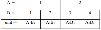
Here is an example of a nested classification. Microbial counts are made on samples of ground beef in a study whose objective is to assess sources of variation in numbers of microbes. Twenty packages of ground beef (PACKAGE) are purchased and taken to a laboratory. Three samples (SAMPLE) are drawn from each package, and two replicate counts are made on each sample. Output 4.1 shows the raw data.

Output 4.1 Microbial Counts in Ground Beef

The data are plotted in Output 4.2, with points identified according to their SAMPLE number.

Output 4.2 Plots of Count versus Package Number

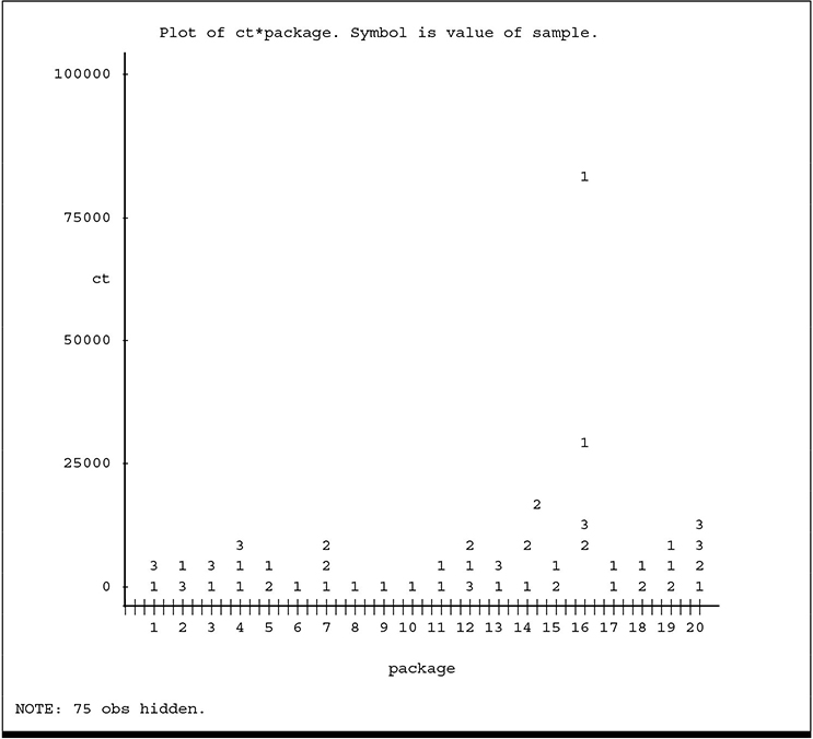
You can see the larger variation among larger counts. In order to stabilize the variance, the logarithm (base 10) of the counts (LOGCT) was computed and serves as the response variable to be analyzed. The plot of LOGCT, which appears in Output 4.3, indicates the transformation was successful in stabilizing the variance.

Output 4.3 Plot of Log Count versus Package Number

Logarithms are commonly computed for microbial data for the additional reason that interest is in differences in the order of magnitude rather than in interval differences.

A model for the data is

y_ijk = μ + a_i + b(a)_ij + e_ijk             (4.1)

where

yijk	is the log10 count for the kth replicate of the jth sample from the ith package.
μ	is the overall mean of the sampled population.
ai	are the effects of packages, that is, random variables representing differences between packages, with variance ${\sigma }_p^2$, i = 1, . . . , 20.
b(a)ij	are random variables representing differences between samples in the same package, with variance ${\sigma }_s^2$, i = 1, . . . ,20, j = 1, 2, 3.
eijk	are random variables representing differences between replicate counts in the same sample, with variance σ2, i = 1, . . . ,20, j = 1, 2, 3 and k = 1, 2.

The random variables a_i, b(a)_ij, and e_ijk are assumed to be normal distributed and independent with means equal to 0. Note several conventions used in this text for denoting fixed versus random effects. Greek symbols denote fixed effects, as they have for all models in previous chapters, and for μ in this model. Latin symbols denote random effects. If you consider packages to be fixed, instead of random, you would denote the package effects as α_i instead of αa_i. The notation b(a) is used for nested factors, in this case factor B (samples) nested within factor A (packages). You could denote the effects of replicates within samples as c(ab)_ijk, but by convention the smallest subunit in the model is generally denoted as e_ijk.

The variance (V) of the log counts can be expressed as

V(y_ijk) = ${\sigma }_y^2$
           = ${\sigma }_p^2$ + ${\sigma }_s^2$ + ${\sigma }_{}^2$

Expressing the equation with words, the variance of the logarithms of microbial count is equal to the sum of the variances due to differences among packages, among samples in the same package, and between replicates in the same sample. These individual variances are therefore called components of variance. The first objective is to estimate the variance components, and there are several statistical techniques for doing so, including analysis of variance (ANOVA) and maximum likelihood (or, more commonly, restricted maximum likelihood, or REML). In this chapter, both ANOVA and REML methods are used. For balanced data, ANOVA and REML produce identical results. The first examples in this chapter use ANOVA because it is easier to see how the method works. PROC MIXED, introduced later in this chapter, uses REML because it is easier to generalize to more complex models.

4.2.1 Analysis of Variance for Nested Classifications

An analysis-of-variance table for the ground beef microbial counts has the following form:

Source of Variation	DF
packages	19
samples in packages	40
replicates in samples	60

You can produce this table by using the GLM procedure (see Chapter 3, “Analysis of Variance for Balanced Data”). You can also use the ANOVA, NESTED, and VARCOMP procedures to produce this table. The MIXED procedure does not compute the analysis of variance table per se, but it computes statistics that are typical end points for the analysis of data with random effects. Which procedure is best to use depends on your objectives.

As noted in Chapter 3, PROC ANOVA computes analysis of variance for balanced data only. PROC GLM computes the same analysis of variance but can be used for unbalanced data as well (see Chapter 5). In the early days of computing, limited capacity often forced users to use PROC ANOVA for large data sets. However, with contemporary computers this is rarely an issue and hence there is rarely any reason to use PROC ANOVA instead of PROC GLM. PROC NESTED is a specialized procedure that is useful only for nested classifications. It provides estimates of the components of variance using the analysis-of-variance method of estimation. Because PROC NESTED is so specialized, it is easy to use. However, PROC GLM can compute the same analysis of variance as PROC NESTED, but it does so within the framework of a much broader range of applications. Finally, PROC MIXED and PROC VARCOMP compute the variance component estimates. The MIXED procedure can also compute a variety of statistics not available with any other procedure. Many of these statistics have become increasingly important in the analysis of data with random effects. For these reasons, this chapter focuses on using PROC GLM to compute the analysis of variance, and later sections introduce PROC MIXED to compute additional statistics typically of interest.

The program statements for PROC GLM are similar to those introduced in Chapter 3. You add a RANDOM statement to compute the expected values of the mean squares—that is, what is being estimated by the individual mean squares. Here are the proper SAS statements:

proc glm;
 class package sample;
 model logct=package sample(package);
 random package sample(package);

You can see that the syntax for a nested effect, in this case SAMPLE nested within PACKAGE, follows from the notation used for nested effects in model (4.1). The RANDOM statement is simply a list of effects in the model to be considered random. In most practical situations, you add a TEST option to the RANDOM statement in order to compute the proper test statistics. Section 4.2.3 illustrates the TEST option. However, you should first understand the analysis-of-variance statistics that PROC GLM computes by default.

The analysis-of-variance results appear in Output 4.4, and the expected mean square coefficients are given in Output 4.5.

Output 4.4 GLM Analysis of Variance of Log Count

Note: The F-statistics computed by PROC GLM for the basic analysis of variance of models with random effects are not necessarily correct. For the basic F-statistics shown above, GLM always uses MS(ERROR) for the denominator. For example, the F-statistic for PACKAGE is incorrect because MS(ERROR) is not the correct denominator mean square. Section 4.2.3, in conjunction with Table 4.1, shows you how to use the expected mean squares to determine the correct F-statistics.

Output 4.5 Expected Mean Squares for Log Count Data

Now consider the output labeled “Type III Expected Mean Square.” This part of the output gives you the expressions for the expected values of the mean squares. Table 4.1 shows you how to interpret the coefficients of expected mean squares.

Table 4.1 Coefficients of Expected Mean Squares

Variance Source	Source of Variation	DF	Expected Mean Squares	This Tells You:
PACKAGE	packages	19	${\sigma }_{}^2$ + 2${\sigma }_s^2$ + 6${\sigma }_p^2$	MS(PACKAGE) estimates
				${\sigma }_{}^2$ + 2${\sigma }_s^2$ + 6${\sigma }_p^2$
SAMPLE	samples in packages	40	${\sigma }_{}^2$ + 2${\sigma }_s^2$	MS(SAMPLE) estimates
				${\sigma }_{}^2$ + 2${\sigma }_s^2$
ERROR	replicates in samples	60	${\sigma }_{}^2$	MS(ERROR) estimates
				σ2

From the table of coefficients of expected mean squares you get the estimates of variance components. These estimates are

❏ ${\widehat{\sigma }}^2$ = 0.0385 = MS(ERROR)

❏ ${\widehat{\sigma }}_{{}^s}^2$ = 0.2299 = [MS(SAMPLE) – MS(ERROR)]/2

❏ ${\widehat{\sigma }}_{{}^p}^2$ = 0.1847 = [MS(PACKAGE) – MS(SAMPLE)]/6

The variance of a single microbial count is

${\widehat{\sigma }}_{{}^y}^2$ = TOTAL Variance Estimate

                      = ${\widehat{\sigma }}_{{}^{}}^2$ + ${\widehat{\sigma }}_{{}^s}^2$ + ${\widehat{\sigma }}_{{}^p}^2$
                      = 0.0385 + 0.2299 + 0.1847
                      = 0.4532

Note: The expression TOTAL Variance Estimate does not refer to MS(TOTAL) = 0.4435,

       although the values are similar. From these estimates, you see that

❏ 8.49% of TOTAL variance is attributable to ERROR variance

❏ 50.74% of TOTAL variance is attributable to SAMPLE variance

❏ 40.77% of TOTAL variance is attributable to PACKAGE variance.

4.2.2 Computing Variances of Means from Nested Classifications and Deriving Optimum Sampling Plans

The variance of a mean can also be partitioned into portions attributable to individual sources of variation. The variance of a mean ${\bar{Y}}_{\cdot \cdot \cdot }$ computed from a sample of n_P packages, n_S samples per package, and n replicates per sample, is estimated to be

${\widehat{\sigma }}_{{}^y\mathrm{...}}^2$ = ${\widehat{\sigma }}_{{}^p}^2$ / n_p + ${\widehat{\sigma }}_s^2$/n_pn_s + ${\widehat{\sigma }}_{}^2$ / n_pn_sn

Output 4.4 showed that the overall mean is 3.0494. Its standard error can be determined from the square root of the formula for the variance of the mean. For these data, the standard error is

${\widehat{\sigma }}_{{}^y\mathrm{...}}^2$ = [(0.1847)/20 + (0.2299) / 20 * 3 + (0.0385) / 20 * 3250 * 2] ^(1/2) = 0.1157

The formula for the variance of a mean can also be used to derive an optimum sampling plan, subject to certain cost constraints. Suppose you are planning a study, for which you have a budget of $500. Each package costs $5, each sample costs $3, and each replicate count costs $1. The total cost is

cost = $5 * n_p+ $3 * n_p * n_s+ $1 * n_p * n_s * n

You can create a SAS data set by taking various combinations of n_P, n_S, and n for which the cost is $500, and compute the variance estimate for the mean. Then you can choose the combination of n_P, n_S, and n that minimizes ${\widehat{\sigma }}_{{}^y\mathrm{...}}^2$

4.2.3 Analysis of Variance for Nested Classifications: Using Expected Mean Squares to Obtain Valid Tests of Hypotheses

Expected mean squares tell you how to set up appropriate tests of a hypothesis regarding the variance components. Suppose you want to test the null hypothesis H₀: ${\sigma }_p^2=\text{0}$. If this null hypothesis is true, then the expected mean square for PACKAGE and the expected mean square for SAMPLE (samples in packages) are both equal to ${\sigma }^2+2{\sigma }_s^2$. Therefore, MS(PACKAGE) and MS(SAMPLE) should have approximately the same value if H₀: ${\sigma }_p^2=\text{0}$ is true. On the other hand, if H₀: ${\sigma }_p^2=\text{0}$ is false, then the MS(PACKAGE) should be larger than the MS(SAMPLE). It follows that you can compare the value of MS(PACKAGE) with the value of MS(SAMPLE) to get an indication of whether the null hypothesis is true or false.

Formally, you do this with an F-statistic: divide MS(PACKAGE) by MS(SAMPLE). The result has an F-distribution with n_p –1 DF in the numerator and n_p(n_s–1) DF in the denominator. For the microbial count data, F=1.607/0.498=3.224, with numerator DF=19 and denominator DF=40, which is significant at the p=0.0009 level. Therefore, you reject H₀: ${\sigma }_p^2=\text{0}$, and conclude ${\sigma }_p^2>0$.

You can go through the same process of using the table of expected mean squares to set up a test of the null hypothesis H₀: ${\sigma }_s^2=0$. You see that the appropriate test statistic is F=MS(SAMPLE)/MS(REPLICATE), with numerator DF=40 and denominator DF=60. This F=12.952 is significant at the p<0.0001 level. Again, you conclude ${\sigma }_p^2>0$.

You can compute the test statistics for H₀: ${\sigma }_p^2=0$ and H₀: ${\sigma }_s^2=0$ using PROC GLM. Either you can use the TEST option with the RANDOM statement, or you can use a TEST statement to define the F-statistic you want to use. The needed SAS statements are

proc glm;
 class package sample;
 model logct=package sample(package);
 random package sample(package)/test;
 test h=package e=sample(package);

Notice that you only need to use either the TEST option in the RANDOM statement or the TEST statement, but not both. The former uses the expected mean squares determined by the RANDOM statement to define the appropriate F-statistics. The latter requires you to know what ratio needs to be computed. In the TEST statement, H= refers to the numerator MS, and E= specifies the denominator MS to be used for the F-statistic. For the balanced data sets presented in this chapter, the F-statistics computed by the RANDOM statement’s TEST option and by the TEST statement are the same. This is not always true for unbalanced data, which is discussed in Chapters 5 and 6. Note that you do not need a TEST statement for H₀: ${\sigma }_s^2=0$ because the default F-ratio MS[SAMPLE(PACKAGE)] / MS(ERROR) is correct. Output 4.6 gives the results for the RANDOM statement TEST option and the TEST statement.

Output 4.6 RANDOM TEST Option and TEST Statement Results in PROC GLM for Log Count Data

4.2.4 Variance Component Estimation for Nested Classifications: Analysis Using PROC MIXED

PROC MIXED is SAS’ most sophisticated and versatile procedure for working with models with random effects. You can duplicate the tests and estimates discussed in previous sections. In addition, there are several linear models statistics that only PROC MIXED can compute. This section introduces the basic features of PROC MIXED for random-effects models. The required statements for model (4.1) are

proc mixed;
  class package sample;
  model logct= ;
  random package sample(package);

In some respects, the statements for PROC GLM and PROC MIXED are the same—the CLASS statement, the MODEL statement up to the left-hand side, and the RANDOM statement are all identical to the statements used above for PROC GLM. The MODEL statement contains the big difference. In PROC GLM, you list all the effects in the model other than the intercept and error, regardless of whether they are fixed or random. In PROC MIXED, you list ONLY the fixed effects, if there are any, other than the intercept. For this model, the only fixed effect is ?, so nothing appears to the right of the equal sign except a space and a semicolon. Output 4.7 shows the results for these statements.

Output 4.7 Basic PROC MIXED Results for Log Count Data

The essential part of this output appears under “Covariance Parameter Estimates.” These are the estimates of ${\sigma }_p^2\text{, }{\sigma }_s^2\text{, and }{\sigma }^{\text{2}}$, the PACKAGE, SAMPLE(PACKAGE), and RESIDUAL (or error) variances. You can see that they are the same as the estimates obtained using the analysis of variance and expected mean squares in Section 4.2.1. This will always be true for balanced data, but not necessarily for unbalanced data. Chapter 5 presents examples with unbalanced data. PROC MIXED uses restricted maximum likelihood, usually referred to by its acronym, REML, to estimate variance components. Chapter 6 contains a brief explanation of REML and gives references for additional information.

The REML procedure requires numerical iteration. The “Iteration History” appears immediately before the variance component estimates. You should look for the expression “Convergence Criteria Met.” If it appears, fine. For the types of data sets in this book, convergence problems are extremely rare. If you do get a failure to converge, it is probably because the data are being misread, or the CLASS, MODEL, or RANDOM statements are mistyped.

The basic MIXED output does not contain an analysis-of-variance table. If you want to test hypotheses about the variance components, you can use PROC GLM to compute the F-tests as shown previously. PROC MIXED does allow you two ways to test the variance components—the Wald test and the likelihood ratio test. Of the two, the likelihood ratio test is preferable for most applications.

The likelihood ratio test uses the residual log likelihood—more precisely, –2 times the residual log likelihood, that is, “–2 Res Log Likelihood” in Output 4.7—to construct a test statistic that has an approximate χ² distribution. For the model that contains both effects, PACKAGE and SAMPLE(PACKAGE), the –2 residual log likelihood is 128.2. If you drop SAMPLE(PACKAGE) from the RANDOM statement and rerun the analysis, you can test H₀: ${\sigma }_s^2=0$. Run the SAS statements

proc mixed;
  class package sample;
  model logct= ;
  random package;

You get the “Fit Statistics” shown in Output 4.8.

Output 4.8 Statistics for Fit of Model without SAMPLE (PACKAGE) for Log Count Data

The –2 residual log likelihood for this model is 201.2. The difference between this and the value of the full model is 201.2–128.2 = 73.0. This is the likelihood ratio statistic. It has an approximate χ² distribution with 1 DF. The 1 DF is because one variance component has been removed from the model. The α=0.05 critical value for χ² is 3.84, the p-value for χ²=73.0 is <0.0001. Therefore, you reject H₀: ${\sigma }_s^2=0$.

You can then drop PACKAGE from the model to test H₀: ${\sigma }_p^2=0$. The statements

proc mixed;
  class package sample;
  model logct= ;

yield a –2 residual log likelihood of 245.7. The likelihood ratio test statistic for H₀: ${\sigma }_p^2=0$ is 245.7–201.2 = 44.5. Again, comparing it to ${\chi }_{(1)}^2$ shows that you reject H₀. The p-value is <0.0001.

You can also obtain Wald statistics. You use the option COVTEST in the PROC MIXED statement to compute approximate standard errors for the variance components. The Wald statistic is the ratio $Z=\frac{\text{variance estimate}}{\text{standard error}}$. Z is assumed to have an approximate standard normal distribution. Use the following SAS statements:

proc mixed covtest;
  class package sample;
  model logct= ;
  random package sample(package);

Output 4.9 shows the results.

Output 4.9 PROC MIXED Variance Component Estimates Using the COVTEST Option

Using H₀: ${\sigma }_p^2=0$ as an example, the asymptotic standard error of ${\widehat{\sigma }}_p^2$ is 0.08885 and thus the approximate Z-statistic is $\frac{0.1847}{0.08885}=2.08$. You can compare Z = 2.08 to a table value from the standard normal distribution, or note that the p-value (Pr>Z) is 0.0188.

Important Note: For tests of variance components, the normal approximation is very poor unless the sample size (in this case the number of packages) is in the hundreds or, preferably, thousands. For this reason, use of the Wald statistic to test variance components is strongly discouraged unless your sample size is very large. The ANOVA F-tests using PROC GLM are preferable. Alternatively, you can construct likelihood ratio tests using PROC MIXED, although doing so requires multiple runs and is therefore less convenient. See Littell et al. (1996) for more about likelihood ratio tests.

4.2.5 Additional Analysis of Nested Classifications Using PROC MIXED: Overall Mean and Best Linear Unbiased Prediction

Section 4.2.2 presented the estimate and standard error of the overall mean. The PROC GLM output provides the estimate y̅…, but not the variance component estimates. You have to calculate these from the mean squares and then hand-calculate the standard error of the mean. PROC MIXED does not compute these numbers by default, but you can obtain them either with the SOLUTION option in the MODEL statement or with an ESTIMATE statement. The SAS statements are

model logct= / solution;
  random package sample(package);
  estimate 'overall mean' intercept 1;

Output 4.10 shows the results.

Output 4.10 PROC MIXED Estimates of Overall Mean for Log Count Data

You can see that the SOLUTION option and the ESTIMATE statement produce identical results. In this case, they are simply different ways of including μ̂ in the output.

In some applications with random-effects models, the equivalent of treatment means may be of interest. Henderson (1963,1975) first developed this procedure in the context of animal breeding. Random sires were used to estimate variance components that had genetic interpretations. At the same time, breeders wanted to assess the “breeding value” of each sire, conceptually similar to the mean sire performance. However, because sire effects are random, and there is information about their probability distribution, this affects how you estimate breeding value. The mixed-model procedure called best linear unbiased prediction, or BLUP, was developed for this purpose. In addition to animal breeding, there are many other applications of BLUP. In clinical trials, random samples of patients provide estimates of the mean performance of a treatment for the population of inference, but BLUPs are essential for physicians to monitor individual patients. In quality assurance, a sample of workers can provide estimates of the mean performance of a machine, but BLUPs can help supervisors monitor the performance of individual employees.

To illustrate using the log count data, suppose you want to know the “mean” log count of the first package (PACKAGE=1 in the SAS data set). In terms of model (4.1) you want to estimate μ+a₁, that is, the overall mean plus the effect of package 1. If PACKAGE were a fixed effect, you would simply calculate the sample mean for package 1, ${\bar{y}}_{1\cdot \cdot }=\text{2}\text{.8048}$. However, because the package effect a₁ is a random variable, its probability distribution must be taken into account, which the sample mean does not do. Instead, you compute the BLUP.

The best linear predictor of μ+a₁ is equal to the estimate of μ + E(a₁|y), the expected value of the effects of package 1 given the data. Because μ is a fixed effect, its estimate, as you have seen, is its sample mean. The conditional expectation of a₁ turns out to be E(a₁)+$\text{cov(}{\widehat{a}}_{\text{1}},{\bar{y}}_{1\cdot \cdot }\text{)[var(}{\bar{y}}_{1\cdot \cdot }{\text{)]}}^{\text{-1}}\text{(}{\bar{y}}_{1\cdot \cdot }-{\bar{y}}_{\cdot \cdot \cdot })$. From model (4.1), E(a₁)=0. The resulting expression is equal to

$\left(\frac{{\widehat{\sigma }}_p^2}{{\widehat{\sigma }}_p^2+\frac{{\widehat{\sigma }}_s^2}{n_s}+\frac{{\widehat{\sigma }}^2}{n_{s}n}}\right)({\bar{y}}_{1\cdot \cdot }{\bar{y}}_{\cdot \cdot \cdot })=\left(\frac{0.1847}{0.1847+\frac{0.2299}{3}+\frac{0.03848}{3*2}}\right)(2.8048-3.0495)=-0.1688$

This expression is often called an “EBLUP” because it uses estimated variance components. A “true” BLUP assumes the variance components are known. Note that the “usual” fixed effects estimate of the package effect, ${\bar{y}}_{1\cdot \cdot }-\bar{y}\cdot \cdot \cdot$ = –0.2447, but EBLUP is smaller. In effect, the estimate of a₁ is shrunk to account for its probability distribution. For this reason, the BLUP is often called a shrinkage estimator.

You can obtain EBLUPs for the random effects, such as ${\widehat{a}}_{\text{1}}$, using a SOLUTION option with the RANDOM statement, and for linear combinations of fixed or RANDOM effects, such as $\widehat{\mu }+{\widehat{a}}_{\text{1}}$, using the ESTIMATE statement. Use the following SAS statements:

proc mixed;
  class package sample;
  model logct= / solution;
  random package sample(package)/solution;
  estimate 'pkg 1 blup' intercept 1 | package 1 0;

Output 4.11 gives the results for the PACKAGE random effects and PKG 1 BLUP, the EBLUP analog of the PACKAGE 1 mean. The SOLUTION statement also causes the SAMPLE(PACKAGE) EBLUPs to be printed, but these are not shown. Note: When random effects are involved, the ESTIMATE statement requires a vertical bar (|). Fixed effects (for example, μ) go before the bar; random effects (for example, a_i) go after the bar. Otherwise, you use the same syntax as in any other ESTIMATE statement.

Output 4.11 EBLUPs of Package Effects and Package “Mean” for Log Count Data

Note that the PKG 1 BLUP is $\widehat{\mu }+{\widehat{a}}_{\text{1}}$ = 3.0495–0.1688. Consistent with the idea of shrinkage estimation, that is, using what is known about the distribution of the package effects, the estimate is “shrunk” toward the overall mean relative to the package 1 sample mean, 2.8048.

4.3 Blocked Designs with Random Blocks

Chapter 3 presented the analysis of variance for randomized-complete-blocks designs. The analysis implicitly assumed fixed blocks. In many cases, it is more reasonable to assume that blocks are random. Technically, the question of fixed versus random blocks depends on whether the blocks observed constitute the entire population of possible blocks—if so, they are fixed. Also considered is whether it is reasonable to assume there is a larger population of blocks with some probability distribution of block effects and the blocks observed are representatives of that population—if so, blocks are random. Seen from this perspective, it is hard to imagine a fixed-block experiment of any inferentially interesting consequence. From a practical viewpoint, however, many experiments do not represent the population of blocks well enough to make use of the additional inference possible with random blocks. Furthermore, with complete-blocks designs, inference for treatment differences is identical for fixed-blocks and random-blocks models. As you will see in Chapters 5 and 6, even when you have missing data or use an incomplete blocks design, fixed versus random typically has only a trivial effect on inference about treatment differences. Thus, for experiments whose exclusive goal is to estimate treatment effects, there is often little point in fulfilling the extra design requirements for random-blocks inference.

On the other hand, if estimating treatments means is important, especially obtaining confidence intervals for means, then the choice of a fixed- or random-blocks model matters a great deal.

The purpose of this section is to present the random-blocks analysis of the randomized-complete-blocks design, and to compare it with fixed-blocks ANOVA. Section 4.3.1 takes the data first presented in Output 3.17 and shows how to use PROC MIXED to do the random-blocks analysis. Section 4.3.2 discusses differences and similarities between the random-blocks analysis and fixed-blocks ANOVA. Section 4.3.2 also presents general guidelines for deciding whether fixed- or random-blocks analysis is more appropriate.

4.3.1 Random-Blocks Analysis Using PROC MIXED

The analysis of variance for the randomized-blocks design uses the model equation

$y_{ij}=\mu +{\tau }_i+{\beta }_j+e_{ij}$          (4.2)

where

yij	is the observation on treatment i and block j.
μ	is the intercept.
τi	is the ith treatment effect.
μj	is the jth block effect.
eij	is the residual, or error, for the ijth observation, assumed i.i.d. N(0,σ2).

The Valencia orange data set presented in Output 3.17 was an example. The τ_i’s were the IRRIG method effects.

The analysis of variance presented in Section 3.5 implicitly assumes that treatments are fixed effects, but it does not depend on any assumptions about the block effects. However, additional features of the analysis of variance using PROC GLM reveals GLM computations assume fixed blocks. Although fixed treatments is usually a reasonable assumption, fixed blocks may not be.

Model (4.2) can be modified for random blocks. Usually, blocks are assumed i.i.d. N(0, ${\sigma }_b^2$). In keeping with the Greek-fixed, Latin-random convention, the block effect μ_j is changed to b_j, so the model equation becomes y_ij = μ + τ_i + b_j + e_ij. Also, the block and error effects are assumed to be mutually independent. Note that the random-blocks model for the randomized-blocks design is a mixed model because it contains both fixed- and random-model effects.

You use the following PROC MIXED statements to compute the mixed-model random-blocks analysis:

proc mixed;
  class bloc irrig;
  model fruitwt=irrig;
  random bloc;

Compared to the GLM statements in Section 3.5, you delete BLOC from the MODEL statement and add a RANDOM statement for the BLOC effect. Output 4.12 shows the results.

Output 4.12 Random-Blocks Analysis of Valencia Orange Data Using PROC MIXED

The output contains the essential information contained in the analysis of variance, but in different form. Instead of sums of squares and mean squares for the various sources of variation, the output provides variance estimates for random-effects sources of variation and F-statistics and associated degrees of freedom and p-values for fixed-effects sources of variation. Note that F=3.27 and p=0.0254 are identical to the results for IRRIG in the analysis of variance (Output 3.18).

You can compute least-squares means (LS means) and estimated treatment differences by adding the statement

lsmeans irrig / diff;

to the above PROC MIXED program. Output 4.13 shows the results.

Output 4.13 Estimated Least-Squares Means and Treatment Differences Using PROC MIXED

For balanced data, LS means for treatments are identical to sample treatment means obtained from the MEANS statement in PROC GLM. Note that the values in the “Estimate” column for the LS means are the same as the IRRIG means in Output 3.19. The output from PROC MIXED gives the standard error of the estimated treatment means by default. Here, the standard error is 42.0652. The standard error of a treatment mean in the random-blocks analysis of a randomized-complete-blocks design is $\sqrt{\frac{{\widehat{\sigma }}_b^2+{\widehat{\sigma }}^2}{r}}$ where r is the number of blocks. In this case, the standard error is $\sqrt{\frac{10793+\text{3362}\text{.38}}{8}}$ since ${\widehat{\sigma }}_b^2=10793$, ${\widehat{\sigma }}^2=3362.38$, and r=8. The “Differences of Least Squares Means” table gives the estimated differences, their standard errors, t-statistics and their associated p-values. Note that by definition the t-statistics are least significant difference (LSD) tests for pairwise differences. For randomized-complete-blocks designs, the standard error of a treatment difference is $\sqrt{\frac{2{\widehat{\sigma }}^2}{r}}$, which for these data equals $\sqrt{\frac{2\times 3362.38}{8}}=28.993$. You can calculate the LSD statistic by multiplying the standard error of the difference by t_{(α, dfe}), the table value of the t-distribution for the error degrees of freedom (DFE) and the desired α-level. For example, for these data, DFE=28, hence t_(α=0.05,28)=2.048. Thus, the LSD statistic is 28.993 2.048=59.378, the same (aside from rounding error) as appears in Output 3.19.

As with the MEANS statement in PROC GLM, you can specify mean comparisons other than the LSD test. The ADJUST= option with the LSMEANS statement in PROC MIXED allows you to adjust the p-value to correspond to different procedures. For example, use these statements to compute p-values for Dunnett’s test:

proc mixed order=data;
  class bloc irrig;
  model fruitwt=irrig;
  random bloc;
  lsmeans irrig/diff adjust=dunnett;

Ordinarily, you do not need to use the ORDER=DATA option in the PROC MIXED statement; it is a special requirement for Dunnett’s test with this example. From the description of the problem in Chapter 3, the FLOOD method was intended to be the reference. As with PROC GLM, the default control or reference treatment for the DUNNETT test is the first treatment in alphameric order. In Section 3.5, you used an option with the MEANS statement in PROC GLM to override this default. However, there is no corresponding option in the LSMEANS statements in GLM or MIXED. In order to obtain the desired test, you have to rearrange the data as they are entered in the DATA step so that the FLOOD level of IRRIG appears first, then use the ORDER=DATA option. This changes the order of the treatments for assigning CONTRAST and ESTIMATE coefficients as well as for Dunnett’s test. You can look at the “Class Level Information” (not shown) or the order in which the LS means are printed (shown below) to see the order of the treatments MIXED will use. The results appear in Output 4.14.

Output 4.14 Dunnett-Adjusted p-values for PROC MIXED Analysis of Valencia Orange Data with FLOOD as the Control Irrigation Method

Note the order that the IRRIG levels appear in the “Least Squares Means” table follows from the order the data were entered and the ORDER=DATA option in the PROC MIXED statement. FLOOD was entered first, then the other IRRIG levels in alphabetical order. The “Differences of Least Squares Means” shows only differences allowed by Dunnett’s test with FLOOD as the reference treatment. Two sets of p-values are shown. The first are the unadjusted t-test results, identical to what you would get in an LSD test. The “Dunnett-Hsu” adjustment are the appropriate p-values for Dunnett’s test.

In Section 3.5, standard errors were not discussed. Least-squares means and their standard errors can be obtained in conjunction with analysis of variance using the LSMEANS statement in PROC GLM. However, GLM does not allow you to compute standard errors of treatment differences, as you can with the DIFF option in MIXED. In addition, GLM and MIXED compute different standard errors for the LS means, revealing the primary distinction between fixed-blocks and random-blocks analysis. The next section discusses these differences.

4.3.2 Differences between GLM and MIXED Randomized-Complete-Blocks Analysis: Fixed versus Random Blocks

For randomized-complete-blocks designs, inference on treatment differences is entirely unaffected by whether blocks are fixed or random. This is not true with missing data or incomplete-blocks-designs (see Chapter 6). However, for inference on treatment means, standard errors, and hence how you interpret the data, can be substantially affected by fixed versus random blocks.

4.3.2.1 Treatment Means

You can obtain LS means and their standard errors in PROC GLM using the statement

lsmeans trt / stderr;

Unlike PROC MIXED, GLM does not compute the standard error by default. You must use the STDERR option. The results appear in Output 4.15.

Output 4.15 LS Means for Analysis of Randomized-Complete-Blocks Design Using PROC GLM

Note the return to the original order of the data. The LS means are the same as computed by MIXED (Output 4.13) and by the MEANS statement in PROC GLM (Output 3.19). However, whereas MIXED obtained a standard error of 42.0652, the standard error of the mean using GLM is 20.5012. Why the difference? PROC GLM uses the fixed-block formula for the standard error of the mean, $\sqrt{\frac{{\widehat{\sigma }}^2}{r}}=\sqrt{\frac{\text{MS(error)}}{r}}=\sqrt{\frac{3362.38}{8}}=20.5012$. In fact, PROC GLM’s programming assumes all model effects are fixed. Chapter 6 presents the theory underlying PROC GLM in greater detail. While the RANDOM statement allows GLM to determine expected mean squares and to select appropriate mean square ratios accordingly to construct F-statistics, the RANDOM statement does not affect the way GLM computes standard errors. If you add a RANDOM statement to the GLM program for these data, it will compute expected mean squares, but the standard error of the LS means will remain 20.5012.

With fixed blocks, the definition of a treatment LS mean for the randomized-blocks design is $\mu +{\tau }_i+\frac{1}{r}{\displaystyle \sum _j{\beta }_j}$. With fixed blocks, all uncertainty about the treatment mean is assumed to result from variation among experimental units within a block. With random blocks, the treatment LS Mean is defined as μ + τ_i. Therefore, variation among blocks and variation among units within a block contribute to uncertainty. You can use the following ESTIMATE statements with PROC MIXED for more insight:

estimate 'irrig lsmean' intercept 1 irrig 1 0;
estimate 'irrig narrow lsm' intercept 8 irrig 8 0
       | bloc 1 1 1 1 1 1 1 1/divisor=8;

The first ESTIMATE statement uses the coefficients from the definition of the LS mean for BASIN in a random-blocks model. The second uses the fixed-blocks definition of the LS mean for BASIN. Note that for the random-blocks model, the second ESTIMATE statement is actually a BLUP. More precisely, it is a BLUP limiting the estimate of the treatment mean to only those blocks actually observed. Hence, it is termed the “narrow” estimate, because it narrows the scope of inference from the entire population of blocks to only the blocks that were observed. Output 4.16 shows the results.

Output 4.16 BASIN LS Mean: Usual Definition and Narrow Inference Definition from the ESTIMATE Statement in Random-Blocks Analysis

The numbers in the “Estimate” column reflect a MIXED round-off idiosyncrasy—they are both 290.375, the same as the LS mean and the MEANS in PROC GLM. The standard error of the first estimate matches the MIXED LS mean; the second matches GLM.

To summarize, the standard error that PROC GLM obtains—that is, the fixed-blocks standard error of the mean—assumes that all uncertainty in the estimated treatment means results exclusively from experimental unit variability. The random-blocks standard error that PROC MIXED obtains assumes that there is additional variation among blocks, over and above experimental unit differences.

One way to view this is to assume you want to use the information from this study to anticipate the mean fruit weight yield you will get at your orchard. The estimated mean for the BASIN treatment is 290.375. You know you will not have a mean yield of exactly 290.375, so you want to put a confidence interval around this estimate. How wide should it be? If you use the fixed-blocks standard error for your confidence interval, you assume your orchard has the same expected yield as the orchards used in the experiment. Only variation among the plots contributes to uncertainty. If you use the random-blocks standard error, you assume your orchard is different from the orchards used in the experiment, and that there is likely to be variation among orchards in addition to variability within the orchard. The block variance is the best measure you have of the variance among orchards.

The validity of the random-blocks confidence interval depends on this last sentence. Does the block variance really provide an adequate estimate? Typically, if the blocks are in close proximity and intended mainly to account for local variation, the answer is probably no. On the other hand, if the blocks do a reasonably good job of representing variability in the population, then the block variance can provide the basis for a useful confidence interval for the mean. This latter condition occurs when the blocks are locations, operators, batches, or similar effects, and a plausible, even if not technically random, sampling scheme has been used.

4.3.2.2 Treatment Differences

For fixed blocks, the expected value of the treatment mean is $\mu +{\tau }_i+\frac{1}{r}{\displaystyle \sum _j{\beta }_j}$. For random blocks, the expected value is μ + τ_i. The LS mean definitions used in the last section follow from these expectations. Under either definition, the estimate of the treatment mean is τ_i − τ_i′, for any pair of treatments i ≠ i´. Therefore, the standard error of a difference is not affected by the question of fixed versus random blocks. It follows that all treatment comparisons, for example, orthogonal contrasts, are similarly unaffected. Unlike PROC MIXED, there is no option in the LSMEANS statement in PROC GLM to compute the standard error of a difference. However, you can use the ESTIMATE statement in PROC GLM. For example, for the Valencia orange data, you can use the statement

estimate ‘trt diff’ irrig 1 –1 0;

to compute the estimate and standard error of the difference between the BASIN and FLOOD treatments. In a complete-blocks design, the standard errors for all pairwise differences are equal, so it is sufficient to compute just one. Output 4.17 shows the result.

Output 4.17 Estimate and Standard Error of Treatment Difference Using the GLM ESTIMATE Statement

You see that the standard error of the difference is identical to that obtained using PROC MIXED for the random-blocks model.

For this reason, just because a design is not suitable for allowing a valid interval estimate of treatment means, this does not mean that it is necessarily unsuitable for obtaining valid interval estimates of treatment differences. Because treatment difference estimates do not depend on fixed versus random-blocks issues, well-conceived block designs can always provide valid estimates of treatment effects. However, the requirements for a blocked design to provide believable interval estimates of treatment means are more exacting. Specifically, if you want good interval estimates of the treatment means, ideally you need a random sample of the population of blocks. Failing that, you at least need a sample that plausibly represents variation among blocks in the population.

4.4 The Two-Way Mixed Model

Recall the discussion in Section 3.7, “A Two-Way Factorial Experiment.” Assume that you actually have sources of seed from many varieties, perhaps several hundred. Also, suppose the objective of the experiment is to compare the methods across all the varieties in the population of potential varieties. Because it is not feasible to include all varieties in the experiment, you randomly choose a manageable number of varieties—say, five, for the purposes of this example—from the population of varieties. Your interest is not specifically in these five varieties, but in the population from which they were drawn. This makes VARIETY a random effect. As a consequence, any effect involving VARIETY is also a random effect. In particular, METHOD*VARIETY is a random effect. Interest remains only in the three methods, so METHOD is still a fixed effect. Since both random and fixed effects are involved, the model is mixed.

The fact that VARIETY is a random effect alters how you should analyze METHOD differences. First of all, VARIETY being a random effect determines how you measure experimental error appropriate for comparing methods. Furthermore, in many applications, you are not interested in simple effects, but only in METHOD main effects. When the response of specific VARIETY levels or simple effects of METHOD given VARIETY are of interest, you must take into account the distribution of VARIETY and METHOD*VARIETY effects. As you saw in Section 4.2, the means you use are EBLUPs.

You can test the main effect of METHOD either by using PROC GLM with the RANDOM statement and TEST option to determine the appropriate F-statistics, or by using PROC MIXED. You can use both PROC MIXED and, up to a point, PROC GLM, to do mean comparison tests. Only PROC MIXED can compute correct standard errors for all the means and differences of potential interest. Also, PROC GLM cannot compute EBLUPs; when they are of interest, you must use PROC MIXED.

4.4.1 Analysis of Variance for the Two-Way Mixed Model: Working with Expected Mean Squares to Obtain Valid Tests

A model for the data is

y_ijk = μ + α_i + b_j + (ab)_ij + e_ijk

where

μ + αi= μi	is the mean for method i, averaged across all varieties in the population, i =1, 2, 3.
bj	are random variables representing differences between varieties, assumed i.i.d. N(0, ${\sigma }_V^2$); j = 1,...,5.
(ab)ij	are random variables representing interaction between methods and varieties, assumed i.i.d. N(0, ${\sigma }_{MV}^2$).
eijk	are random variables representing differences in yields among plants of the same variety using the same method, assumed i.i.d. N(0,σ2), with k = 1,...,6.

The random variables b_j, (ab)_ij, and e_ijk are all assumed to be mutually independent.

Note: This formulation of the model is not universally accepted. Other formulations specify other assumptions regarding terms in the model. See Hocking (1973). The main distinction in these formulations pertains to how you define VARIETY variance. This is discussed at greater length in Chapter 6, “Understanding Linear Models Concepts.” Here, the concern is comparing METHODs. All formulations of the model lead to the same techniques for comparing METHODs, so the issue of alternative model formulations is not of immediate concern.

The data contain the same sources of variation whether VARIETY is fixed or random, so you can compute the same analysis-of-variance table. But you should use computations from the table differently than when VARIETY was considered fixed. The main effect of differences between METHODs, rather than simple effects, even in the presence of interaction between METHOD and VARIETY, is tested here. Also tested is the comparison A vs B,C between the METHODs. Now, however, the focus is on the main effect of the contrast, even in the presence of interaction.

Run the following statements:

proc glm data=fctorial; class method variety;
  model yield = method variety method*variety / ss3;
  contrast 'A vs B,C' method 2 -1 -1;

The results appear in Output 4.18.

Output 4.18 Analysis of Variance for the Two-Way Mixed Model

Add the RANDOM statement to specify that VARIETY and METHOD*VARIETY are random effects.

random variety method*variety;

The RANDOM statement specified here only causes expected mean squares to be computed. It does not affect any of the PROC GLM computations. Note that you must place the RANDOM statement after the CONTRAST statement in order to get the expected mean square for the contrast. If you want correct F-statistics, you have to specify them in a TEST statement or use the TEST option in the RANDOM statement.

Output 4.19 shows expected mean squares.

Output 4.19 Expected Mean Squares for Two-Way Mixed Models

In statistical notation, these expected mean squares are as follows:

Source	Expected Mean Squares
METHOD	${\sigma }^2+6{\sigma }_{MV}^2+30[{\displaystyle \sum _i{({\alpha }_i-{\bar{\alpha }}_{\cdot })}^2/2}]$
VARIETY	${\sigma }^2+6{\sigma }_{MV}^2+18{\sigma }_V^2$
METHOD*VARIETY	${\sigma }^2+6{\sigma }_{MV}^2$
ERROR	σ2

You can probably see how all of these terms come from Output 4.19 except for the expression $30[{\displaystyle \sum _i{({\alpha }_i-{\bar{\alpha }}_{\cdot })}^2/2}]$, which corresponds to Q(METHOD) for the METHOD source of variation. You can use the Q option if the RANDOM statement of PROC GLM to obtain output you can then use to obtain this expression. Section 4.4.3 presents a more detailed explanation. For now, all you need to know about Q(METHOD) is that it measures differences between the METHOD means. This is true because μ_i= μ + α_i and therefore, ${\sum }_i{({\alpha }_i-\bar{\alpha }.)}^2={\sum }_i{({\mu }_i-\bar{\mu }.)}^2.$

The null hypothesis H₀: μ_A=μ_B=μ_C is true when Q(METHOD)=0. Therefore, when H₀ is true, the expected mean square for METHOD is the same as the expected mean square for METHOD*VARIETY. This tells you to use F=MS(METHOD)/MS(METHOD*VARIETY) to test the null hypothesis. You can obtain this either by adding the TEST option to the RANDOM statement or by using the following TEST statement:

test h=method e=method*variety;

At first glance, the expected mean square for the contrast A vs B,C in Output 4.19 appears to be the same as the expected mean square for METHOD, but Q(METHOD) has a different interpretation. For the contrast A vs B,C, Q(METHOD) stands for 30[μ_A − 0.5(μ_B + μ_C)]². The form of the contrast expected mean square tells you to use F=MS (A vs B,C)/MS(METHOD*VARIETY) to test the null hypothesis H₀: μ_A–0.5(μ_B+ μ_C)=0. You can do this with the E= option in the CONTRAST statement:

contrast 'A vs B,C' method 2 -1 -1 / e=method*variety;

Results of the TEST and CONTRAST statements appear in Output 4.20.

Output 4.20 Tests Using the Proper Denominator in the F-Statistic

The denominator MS(METHOD*VARIETY) of the F-values in Output 4.20 is larger than the denominator MS(ERROR) of the F-values in Output 4.18. The correct F-tests (Output 4.20) are therefore less significant than they appeared to be using Output 4.18 inappropriately. Using MS(METHOD*VARIETY) in the denominator makes inference from the tests valid for all varieties in the population, whereas use of MS(ERROR) in the denominator restricts inference to only the five varieties actually used in the experiment. MS(METHOD*VARIETY) is the experimental error for comparing methods across all varieties in the population, whereas MS(ERROR) is the experimental error for comparing methods across only those varieties used in the experiment.

4.4.2 Standard Errors for the Two-Way Mixed Model: GLM versus MIXED

While you can obtain valid F-tests for mixed models with PROC GLM, you cannot always obtain valid standard errors. The two-way mixed model is an example of when GLM cannot compute the correct standard errors. The statement

estimate ‘trt diff’ method 1 –1 0;

computes the estimate and standard error of μ_A– μ_B. The result appears in Output 4.21.

Output 4.21 Estimate and Standard Error for Method A-B Difference Computed by PROC GLM

GLM computes the standard error of the difference as $\sqrt{\frac{2{\widehat{\sigma }}^2}{5*6}}=\sqrt{\frac{2*MSE}{30}}=\sqrt{\frac{2*19.65}{30}}=1.14$. This would be correct if MS(ERROR) was the appropriate measure of experimental error, but we know that the correct measure is MS(METHOD*VARIETY). Thus, the standard error should be $\sqrt{\frac{MS(METHOD*VARIETY)}{30}}$ = $\sqrt{\frac{2({\widehat{\sigma }}^2+6{\widehat{\sigma }}_{MV}^2)}{30}}$. PROC GLM does not have an E= option for the ESTIMATE statement, so the correct standard error is unavailable. You must use PROC MIXED to obtain the correct standard error.

Use the following statements to run the analysis with PROC MIXED:

proc mixed data=fctorial;
  class method variety;
   model yield = method;
   random variety method*variety;
   contrast 'A vs B,C' method 2 -1 -1;

Output 4.22 shows the results.

Output 4.22 Analysis of the Two-Way Mixed Model Using PROC MIXED

Compare these results to Outputs 4.18 through 4.21 using PROC GLM. PROC MIXED provides variance component estimates rather than ANOVA sums of squares and mean squares. From the mean squares in Output 4.18 and the expected mean squares in Output 4.19, you can see that MS(VARIETY)=2.845 is less than MS(METHOD*VARIETY), resulting in a negative estimate of ${\sigma }_V^2$. The default for PROC MIXED is to set negative variance components to 0. Thus, in the output, the “Covariance Parameter Estimates” for VARIETY is 0.

Setting ${\text{σ}}_{\text{V}}^{\text{2}}\text{=0}$ affects the REML estimate of ${\sigma }_{MV}^2$. The ANOVA estimate obtained using the mean squares and their expected values from Outputs 4.18 and 4.19 is 4.527, whereas the REML estimate in Output 4.22 is 2.084. This in turn affects F-statistics for METHOD and the A vs B,C contrast. You can see that truncating variance component estimates at zero has a ripple effect on other statistics. Because truncation at zero results in upward bias in variance component estimates, it also causes bias in affected statistics.

Statisticians, quantitative geneticists, and others who use variance component estimates in their work have struggled with the question of how negative variance components should be reported. Some think that negative estimates should be reported as such, whereas others argue that because variance by definition cannot be negative, negative estimates have no meaning and they should be set to zero. Using variance components to construct test statistics adds another dimension to the problem. While you can debate the merits of reporting negative variance components, biased F-statistics and standard errors are clearly to be avoided.

PROC MIXED has a number of options that allow you to get the same variance component estimates and hence the same F-values that PROC GLM computes. The NOBOUND option uses REML computing algorithms, except that it allows negative variance component estimates to remain negative. The METHOD=TYPEn option (n =1, 2, or 3) computes ANOVA estimates based on the expected mean squares that result from TYPE I, II, or III sum of squares. For the balanced data sets presented in this chapter, all these options produce the same results. Chapters 5 and 6 discuss the differences between the various types of SS for unbalanced data. As an example, the following SAS statements use the Type III variance component estimates:

proc mixed method=type3 data=fctorial;
  class method variety;
   model yield = method;
   random variety method*variety;
   contrast 'A vs B,C' method 2 -1 -1;

Output 4.23 shows the results.

Output 4.23 PROC MIXED Analysis Using the METHOD= TYPE3 Option

The output gives you the same expected mean squares obtained by the RANDOM statement in PROC GLM. When you use the METHOD=TYPEn option, the output also contains the ANOVA table: sum of squares, mean squares, and F-statistics. You can see that the “Covariance Parameter Estimates” correspond to the ANOVA estimates. Also, the F-tests for the METHOD main effect and the A vs B,C contrast are now the same as those obtained by using PROC GLM with the properly specified E= option. As mentioned above, for balanced data you can obtain the same variance component estimates and F-statistics with the NOBOUND option:

proc mixed nobound data=fctorial;

You can obtain the estimated treatment means and differences with their correct standard errors. In conjunction with the above PROC MIXED METHOD=TYPEn or NOBOUND option, use the following statement:

lsmeans method/diff;

Output 4.24 shows the results.

Output 4.24 Estimates of Treatment Means and Differences in the Two-Way Mixed Model Using PROC MIXED

Consistent with the formula for the standard error of a difference, $\sqrt{\frac{2({\widehat{\sigma }}^2+6{\widehat{\sigma }}_{MV}^2)}{30}}$ given above, the value in Output 4.23 is $\sqrt{\frac{2*(19.650+6\times 4.527)}{30}}=1.767$. The t-values and their associated p-values are thus valid LSD tests for METHOD main effect differences.

4.4.3 More on Expected Mean Squares: Determining Quadratic Forms and Null Hypotheses for Fixed Effects

In some situations, you may want to obtain detailed information about the hypotheses tested by various F-statistics. In balanced cases, this is rarely an issue, because the hypotheses are obvious from the structure of the ANOVA table or the contrast coefficients. In unbalanced data sets, however, the hypotheses may depend on the type of SS you use and the order of the terms in the model. These are considered in Chapters 5 and 6. The purpose of this section is to show how to use optional PROC GLM output to use fixed-effects quadratic forms to determine what hypothesis a given F-statistic tests. Using balanced data makes it easier to follow the computations. This section is mainly of interest to graduate students who are learning to use quadratic forms and to readers who are familiar with matrix algebra and want to get a deeper insight into the distinctions among the types of SS.

When you obtain expected mean squares, the basic output gives you a “Q” term for the fixed effects. This “Q” stands for quadratic form. For example, Q(METHOD) is the quadratic form for the fixed-effect METHOD in Outputs 4.19 and 4.23. You can obtain detailed information about the meaning of Q(METHOD) by using the Q option at the end of the PROC GLM RANDOM statement. Output 4.25 shows the results of using the Q option.

random variety method*variety / q;

Output 4.25 Quadratic Forms for Method Effects from the Q Option

The Q option prints a matrix of the quadratic form for fixed effects, which tells you

Q(METHOD) = $\frac{\text{α}΄\text{Aα}}{\text{DF}}$

where α'=(α_A, α_B, α_C) is a row vector containing the fixed-effects parameters in the model. A is the matrix of the quadratic form, and DF is the number of degrees of freedom for the effect. You see two matrices printed in Output 4.25, one for the METHOD effect in the analysis-of-variance table and one for the contrast A vs B,C. For the overall METHOD effect, the matrix is

$\text{A=}\left[\begin{array}{ccc}\text{20}& -10& -10\\ -10& 20& -10\\ -10& -10& 20\end{array}\right]$

This tells you the matrix algebraic expression for the quadratic form is

Q(METHOD)= $\left({\text{α}}_{\text{A}},{\text{α}}_{\text{B}},{\text{α}}_{\text{C}}\right)\left[\begin{array}{ccc}20& -10& -10\\ -10& 20& -10\\ -10& -10& 20\end{array}\right]\left[\begin{array}{c}{\text{α}}_{\text{A}}\\ {\text{α}}_{\text{B}}\\ {\text{α}}_{\text{C}}\end{array}\right]\left(\frac{1}{2}\right)$

Some algebraic manipulation yields Q(METHOD) = $30{\displaystyle \sum _i{({\alpha }_i-{\bar{\alpha }}_{\cdot })}^2}/2$, as indicated earlier. You can go through the same process to get the Q(METHOD) expression for the A vs B,C contrast. Using the Q matrix for the contrast A vs B,C, some straightforward but tedious matrix algebra reveals, as indicated above, that Q(A vs B,C) = 30[μ_A − 0.5(μ_B + μ_C)]².

You can use the quadratic form expressions to indicate the null hypothesis tested by an F-statistic with the corresponding mean square as its numerator. To do this, determine the values of the fixed parameters that make Q(METHOD)=0. For the overall METHOD effect, you have already seen that Q(METHOD)=0 whenever α_A = α_B = α_C, or equivalently, whenever μ_A = μ_B = μ_C.

4.5 A Classification with Both Crossed and Nested Effects

Some classifications involve both crossed and nested factors. The example in this section is typical of a study design that is common to many fields of investigation. As you will see by the end of this section, in practical situations, PROC MIXED is better suited to analyze these kinds of data sets. Nonetheless, in order to adequately present the linear model issues associated with these designs, the first part of this section uses PROC GLM.

Output 4.26 presents a data set that illustrates the essential features of designs with crossed and nested factors. An engineer in a semiconductor plant investigated the effect of several modes of a process condition (ET) on the resistance in computer chips. Twelve silicon wafers (WAFER) were drawn from a lot, and three wafers were randomly assigned to each of four modes of ET. Resistance in chips was measured in four positions (POS) on each wafer after processing. The measurement was recorded as the variable RESISTA in a SAS data set named CHIPS.

Output 4.26 Semiconductor Resistance Data

Here are some features of this experiment:

❏ There are two experimental factors, ET and POS, which appear together in all combinations. These factors are crossed because the POS labels 1, 2, 3, and 4 have the same meaning for all levels of ET; POS 1 refers to the same location on a wafer in ET 1 as it does on a wafer in ET 2. The engineer wants to compare mean resistance between levels of ET and between levels of POS. He also wants to determine if differences between levels of ET depend on the value of POS at which they are measured. The data are analyzed in terms of either simple effects or main effects of ET and POS, depending on the presence or absence of interaction between ET and POS. Section 4.5.2 discusses expected mean squares and how to use them to set up appropriate tests for several types of effects.

❏ ET levels are assigned to wafers in a completely randomized design, making WAFER the experimental unit for comparing levels of ET. Wafers are nested within levels of ET.

❏ Levels of POS change between chips on the same wafer, whereas levels of ET change between wafers. So a different measure of experimental error is required to compare positions than is used to compare levels of ET. This is the primary feature that distinguishes this experiment from a standard factorial.

This data set has features of both crossed and nested classification, so it is referred to as crossed-nested. It is similar to a split-plot experiment, with wafer taken as the main-plot unit and chips on a wafer as the sub-plot unit. It also has features in common with repeated-measures experiments, which are discussed in Chapter 9.

A model for the data is

y_ijk = μ + α_i + w_ij + β_k + (αβ)_ik + e_ijk

where y_ijk is the measured resistance at the kth position on the jth wafer in the ith level of ET, i = 1, 2, 3, 4; j = 1, 2, 3; k = 1, 2, 3, 4; μ+α_i+β_k+(αβ)_ik = μ_ik is the mean resistance at position k with ET level i. w_ij are random variables representing differences among wafers assigned to the same level of ET. The w_ij are assumed i.i.d. N(0, ${\sigma }_W^2$). Some writers prefer to use the notation w(a)_ij to emphasize the fact that wafers are nested within levels of ET.

e_ijk are random variables representing differences among chips on the same wafer. The e_ijk are assumed i.i.d. N(0,α²) and independent of the w_ij. The former is a potentially flawed assumption because correlation between chips could depend on their relative proximity on the wafer. If so, then the data should be analyzed using methods appropriate for repeated-measures experiments (see Chapter 9).

4.5.1 Analysis of Variance for Crossed-Nested Classification

An analysis-of-variance table has the form

Source of Variation	DF
ET	3
WAFER(ET)	8
POS	3
ET*POS	9
ERROR = POS*WAFER(ET)	24

 

4.5.2 Using Expected Mean Squares to Set Up Several Tests of Hypotheses for Crossed-Nested Classification

This section illustrates how to set up several types of tests of hypothesis for an experiment of this type. These include tests of the following null hypotheses:

❏ overall main effect of ET        H₀: μ_1⋅ =μ_2⋅ = μ_3⋅ = μ_4⋅

❏ overall main effect of POS     H₀: μ_⋅1 = μ_⋅2 = μ_⋅3 = μ_⋅4

❏ main effect contrast of ET (ET1 vs ET2)              H₀: μ_1⋅ = μ_2⋅

❏ main effect contrast of POS (POS1 vs POS2)     H₀: μ_⋅1 = μ_⋅2

❏ simple effect contrast of POS (POS1 vs POS2 in ET1)     H₀: μ₁₁ = μ₁₂

❏ simple effect contrast of ET (ET1 vs ET2 in POS1)           H₀: μ₁₁ = μ₂₁

You can use the CONTRAST and RANDOM statements in PROC GLM or PROC MIXED to obtain appropriate tests for these effects. Both allow a high degree of flexibility. GLM is better suited for illustrating key features of linear model theory and methods. Primarily because of standard error considerations discussed in Section 4.5.3, MIXED is better suited to the actual analysis of data. For now, we focus on linear model issues via GLM.

The following SAS statements produce the analysis-of-variance table and contrasts:

proc glm data=chips;
  class et wafer pos;
  model resista = et wafer(et) pos et*pos / ss3;
  contrast 'ET1 vs ET2'           et 1 -1 0 0;
  contrast 'POS1 vs POS2'         pos 1 -1 0 0;
  contrast 'POS1 vs POS2 in ET1'  pos 1 -1 0 0 et*pos 1 -1;
  contrast 'ET1 vs ET2 in POS1'   et 1 -1 0 0 et*pos 1 0 0 0 -1;

Note that the simple effect contrasts POS1 vs POS2 in ET1 and ET1 vs ET2 in POS1 use coefficients of ET*POS in addition to their respective main effects. Table 4.2 and the explanation immediately following detail why these terms are necessary. The analysis-of-variance table and CONTRAST statement results appear in Output 4.27.

Output 4.27 Analysis of Variance for Semiconductor Resistance Data

The output contains F-statistics for all effects in the MODEL statement as well as for all of the effects in the CONTRAST statements. Note: These F-statistics use the default MS(ERROR) in the denominator. Remember that in PROC GLM, the RANDOM statement does not override the default use of MS(ERROR). You must examine the expected mean squares to determine which of these automatically computed F-statistics are valid. For all other tests, you must specify an appropriate error term. As with previous examples in this chapter, you can specify appropriate error terms with a TEST statement or by using the TEST option with the RANDOM statement. For CONTRAST statements, use the E= option.

Now, obtain tests for the fixed effects of ET, POS, and ET*POS in the analysis-of-variance table and tests for the effects specified in the CONTRAST statements. Start by obtaining the expected mean squares for all effects. The following statement gives the results in Output 4.28. Recall that this statement must be placed after the CONTRAST statements in the PROC GLM program given above:

random wafer(et);

Output 4.28 Expected Mean Squares for Semiconductor Data

You could use the Q option at the end of the RANDOM statement to get an interpretation of Q(effect) in the expected mean squares. Table 4.2 relates the Q(effect) with the corresponding algebraic expressions in terms of model parameters and means model.

Table 4.2 Q(effect) in Expected Mean Squares

Effect Name	Expression in Output	Algebraic Expression for Q(effect)
ET	Q(ET,ET*POS)	$12{\displaystyle \sum _i[{\alpha }_i}+{(\overline{\alpha \beta })}_{i\cdot }-{\bar{\alpha }}_{\cdot }-{(\overline{\alpha \beta })}_{\cdot \cdot }{]}^2$ = $4{\displaystyle \sum _i[{\mu }_i-{\bar{\mu }}_{\cdot }}{]}^2$
POS	Q(POS,ET*POS)	$12{\displaystyle \sum _j[\beta j}+{(\overline{\alpha \beta })}_{\cdot j}-{\bar{\beta }}_{\cdot }-{(\overline{\alpha \beta })}_{\cdot \cdot }{]}^2=4{[{\mu }_{\cdot j}-{\bar{\mu }}_{\cdot \cdot }]}^2$
ET*POS	Q(ET*POS)	$12{\displaystyle \sum _{ij}[{(\alpha \beta )}_{ij}-(\overline{\alpha \beta }}{)}_{i\cdot }-{(\overline{\alpha \beta })}_{\cdot j}+{(\overline{\alpha \beta })}_{\cdot \cdot }{]}^2$ = $12{\displaystyle \sum _{ij}[{\mu }_{ij}-{\mu }_{i\cdot }}-{\mu }_{\cdot j}+{\mu }_{\cdot \cdot }{]}^2$
ET1 vs ET2	Q(ET,ET*POS)	$12{[{\alpha }_1+{(\overline{\alpha \beta })}_{1\cdot }-{\alpha }_2+{(\overline{\alpha \beta })}_{2\cdot }]}^2=4{[{\bar{\mu }}_{1\cdot }-{\bar{\mu }}_{2\cdot }]}^2$
POS1 vs POS2	Q(POS,ET*POS)	$12{[{\beta }_1+{(\overline{\alpha \beta })}_{\cdot 1}-{\beta }_2+{(\overline{\alpha \beta })}_{\cdot 2}]}^2=4{[{\bar{\mu }}_{\cdot 1}-{\bar{\mu }}_{\cdot 2}]}^2$
POS1 vs POS2 IN ET1	Q(POS,ET*POS)	$12{[{\beta }_1+{(\overline{\alpha \beta })}_{11}-{\beta }_2+{(\overline{\alpha \beta })}_{12}]}^2=4{[{\bar{\mu }}_{11}-{\bar{\mu }}_{12}]}^2$
ET1 vs ET2 IN POS1	Q(ET,ET*POS)	$12{[{\alpha }_1+{(\overline{\alpha \beta })}_{11}-{\alpha }_2+{(\overline{\alpha \beta })}_{12}]}^2=4{[{\bar{\mu }}_{11}-{\bar{\mu }}_{12}]}^2$

It may seem strange that the Q(effect) for ET main effects contains the expression ET*POS within the parentheses. The ET*POS expression is present because the quadratic form is a function of the (αβ) parameters as well as the α parameters. This is because PROC GLM imposes no assumptions on the model parameters, so that ${\bar{\mu }}_{i\cdot }=\mu +{\alpha }_i+{\bar{\beta }}_{\cdot }+{(\overline{\alpha \beta })}_{i\cdot }$ and ${\bar{\mu }}_{\cdot \cdot }=\mu +\bar{\alpha }\cdot +{\bar{\beta }}_{\cdot }+{(\overline{\alpha \beta })}_{\cdot \cdot }$ Consequently, ${\bar{\mu }}_{i\cdot }-{\bar{\mu }}_{\cdot \cdot }={\alpha }_i-{\bar{\alpha }}_{\cdot }+{(\overline{\alpha \beta })}_{i\cdot }-(\overline{\alpha \beta {)}_{\cdot \cdot }}$; that is, differences between means for two levels of ET are functions of the (αβ)_ik parameters as well as the μ_i parameters. The same type of phenomenon holds true for the main effect of POS and the effects in the CONTRAST statements. Note that the quadratic forms of the simple effect contrasts, POS1 vs POS2 in ET1 and ET1 vs ET2 in POS1, correspond to the coefficients you must use in their respective CONTRAST statements.

In each case, you see from the algebraic expression for Q(effect) that the null hypothesis you want to test is H₀: Q(effect)=0. The expected mean squares tell you to use the denominators in the F-statistics as indicated in this table:

Table 4.3 Required Denominator MS for Tests of Effects

Effect	Appropriate Denominator for F-Statistic
ET	MS(WAFER(ET))
POS	MS(ERROR)
ET*POS	MS(ERROR)
ET1 vs ET2	MS(WAFER(ET))
POS1 vs POS2	MS(ERROR)
POS1 vs POS2 in ET1	MS(ERR0R)
ET1 vs ET2 in POS1	Not directly available

For any tests that use MS(ERROR) the F-statistics PROC GLM automatically computes are correct. All others require additional attention. Note that you cannot compute the appropriate test for the ET1 vs ET2 in POS1 contrast using PROC GLM. In fact, you cannot get the correct standard error for the estimate of ET differences for a given POS with PROC GLM either. The method for getting the right test and standard error are explained later in this section and in Section 4.5.3. The correct statistics are easily obtained using PROC MIXED. Section 4.5.4 shows you how to do this. This is the main reason why PROC MIXED is preferred in actual data analysis.

Appropriate F-tests for ET main effect and ET1 vs ET2 contrast are obtained with the statements

test h=et e=wafer(et);
contrast 'ET1 vs ET2' et 1 -1 0 0 / e=wafer(et);

Results appear in Output 4.29.

Output 4.29 F-Tests for ET Effects

Compare F-statistics in Output 4.29 with those in Output 4.27 for these effects.

Alternatively, you can obtain test statistics for effects in the analysis-of-variance table with the TEST option in the RANDOM statement, as follows:

random wafer(et)/test;

Output 4.30 shows the results.

Output 4.30 F-Tests from the TEST Option

Compare results in Output 4.30 with those in Outputs 4.27 and 4.29. Unfortunately, the TEST option does not compute appropriate tests for effects in CONTRAST statements.

There is no appropriate F-test for the contrast ET1 vs ET2 in POS1 directly available. An appropriate denominator for this F-statistic would be an estimate of ${\sigma }^2+{\sigma }_W^2$. There is no source of variation in the analysis-of-variance table whose expected mean square is equal to ${\sigma }^2+{\sigma }_W^2$. But you can combine MS(ERROR) and MS(WAFER(ET)) to get an estimate of ${\sigma }^2+{\sigma }_W^2$. You need amounts of both α² and ${\sigma }_W^2$ in an appropriate denominator for the F-test; you need one unit of each. Of the expected mean squares for ERROR and WAFER(ET), only the expected mean square for WAFER(ET) contains any ${\sigma }_W^2$; in fact, it contains four units of it. You need to multiply MS(WAFER(ET)) by the appropriate constant to produce one unit of ${\sigma }_W^2$, which, of course, is 1/4. This gives $0.25{\sigma }^2+{\sigma }_W^2$, so you need an additional .75σ², which you can get by adding .75MS(ERROR). So an appropriate denominator of the F-statistic for testing for the effect of ET1 vs ET2 in POS1 is

${\widehat{\sigma }}^2+{\widehat{\sigma }}_W^2$ =.75MS(ERROR) + .25MS(WAFER(ET))

       =.75(0.111).25(0.534)

       = 0.217

An appropriate F-statistic for testing H₀: μ₁₁ – μ₂₁= 0 is then

F =MS(ET1 vs ET2 in POS1)/(${\widehat{\sigma }}^2+{\widehat{\sigma }}_W^2$)

    =0.2166/0.217

Here, F is essentially equal to 1.0, indicating that it is nonsignificant. You do not need to refer it to an F-distribution to calculate a p-value to determine its significance, because F must be substantially larger than 1.0 in order to be significant at any meaningful level. Thus, you do not need to know degrees of freedom for the denominator mean square. Normally, however, you would need degrees of freedom in order to assess the level of significance. They can be approximated using Satterthwaite’s formula, which is demonstrated in Section 4.5.3, “Satterthwaite's Formula for Approximate Degrees of Freedom.”

But first, Table 4.4 gives a summary of all the appropriate F-tests from the analysis-of-variance table and CONTRAST statements:

Table 4.4 Summary of F-Test Results from CONTRAST Statements

Effect	Appropriate F-Statistic	Level of Significance
ET	1.037/0.534 = 1.94	0.202
POS	0.376/0.111 = 3.39	0.034
ET*POS	0.090/0.111 = 0.81	0.612
ET1 vs ET2	0.694/0.534 = 1.30	0.287
POS1 vs POS2	0.077/0.111 = 0.69	0.413
POS1 vs POS2 in ET1	0.040/0.111 = 0.36	0.554
ET1 vs ET2 in POS1	0.217/0.217 = 1.00	NS

4.5.3 Satterthwaite’s Formula for Approximate Degrees of Freedom

The denominator of the F-statistic for the contrast ET1 vs ET2 in POS1 is a linear combination of mean squares from the analysis-of-variance table. In general, such a linear combination has properties that approximate those of actual mean squares. The number of degrees of freedom for the linear combination of mean squares can be approximated by using a formula attributed to Satterthwaite (1946). This is the subject of the following discussion.

Let MS1, . . . ,MSk be a set of independent mean squares with respective degrees of freedom DF₁, . . . ,DF_k, and let a₁, . . . ,a_k be a set of known constants. Then the linear combination

MS=a₁ MS₁ + a₂ MS₂ + . . . + a_k MS_k

is a synthetic mean square with approximate degrees of freedom equal to

DF = $\frac{{(\text{MS)}}^{\text{2}}}{\frac{{{\text{(MS}}_{\text{1}})}^2}{{\text{DF}}_{\text{1}}}+\dots +\frac{{({\text{MS}}_{\text{2}})}^2}{{\text{DF}}_{\text{2}}}}$

Applying Satterthwaite's formula, you get

${\widehat{\sigma }}^2+{\widehat{\sigma }}_W^2=\text{0}\text{.75MS(ERROR) + }\text{.25MS[WAFER(ET)]}$

The data used here yield

MS1 = MS(ERROR) = 0.111	DF1 = 24	a1 = .75
MS2 = MS(WAFER(ET)) = 0.534	DF2 = 8	a2 = .25

so

DF = $\frac{{(0.217)}^{\text{2}}}{\frac{{\text{(0}\text{.083})}^2}{\text{24}}+\frac{{(0.134)}^2}{\text{8}}}$
      = $\frac{0.0471}{0.000287+0.002245}$ = 18.6

SAS has an internal function that can evaluate DF with fractional values. For use with published tables, round down to DF=18. This synthetic mean square with DF=18 is useful for several applications. It is an appropriate denominator for any contrast among levels of ET in a given level of POS, such as the comparison ET1 vs ET2 in POS1 shown in Table 4.3. Other examples include the CONTRAST statement

contrast 'ET1,ET2 vs ET3,ET4 at POS2'
     et 1 1 -1 -1 et*pos 0 0 0 0 1 1 -1 -1;

In addition to providing appropriate denominators for F-statistics, it is equally important to use appropriate mean squares when you compute confidence intervals for means or differences between means. Suppose you wanted a confidence interval on the overall mean for ET1, averaged across WAFER and POS. This mean is

y̅_1⋅⋅ = μ + α₁ + w̅_1⋅ + β₁ + (α̅β̅)_1⋅ + e̅_1⋅⋅

The random parts are w̅_1⋅ and e̅_1⋅. Now w̅_1⋅ is the mean of three w_1j’s (w₁₁, w₁₂, and w₁₃), so V(w̅_1⋅) = ${\sigma }_w^2$/B.

Additionally, e_1.. is the mean of twelve e_1jk’s, so V(e̅_1⋅⋅) = α²/12. Therefore, the variance of y̅_1⋅⋅ is

$\begin{array}{c}V({\overline{\text{y}}}_{\mathrm{1..}})=V({\overline{\text{w}}}_{1.})+V({\overline{\text{e}}}_{\mathrm{1..}})\\ ={\sigma }_w^2/3+{\sigma }^2/12\\ =({\sigma }^2+4{\sigma }_w^2)/12\end{array}$

From the table of expected mean squares you have seen that an estimate of V(${\bar{y}}_{1\cdot \cdot }$) is MS(WAFER(ET))/12. So a 95% confidence interval for the mean is

$\begin{array}{l}{\overline{\text{y}}}_{\mathrm{1..}}\pm t_{8,0.025}\times \sqrt{\frac{\text{MS[WAFER(ET)]}}{12}}\hfill \\ =5.632\pm 2.30(0.210)\hfill \\ =(5.14,6.12)\hfill \end{array}$

Similarly, the mean for POS1 averaged across POS and WAFER is

${\overline{y}}_{\mathrm{..1}}=\text{μ+}\overline{\text{α}}.+\overline{\text{w}}\mathrm{..}+{\text{β}}_1+(\overline{\text{αβ}})+{\overline{\text{e}}}_{\mathrm{..1}}$

The variance of y̅_⋅⋅1 is

$V({\overline{\text{y}}}_{\mathrm{..1}})=V(\overline{\text{w}}\mathrm{..})+V({\overline{\text{e}}}_{\mathrm{..1}})$
             $={\sigma }_w^2/12+{\sigma }^2/12$
             $=({\sigma }_w^2+{\sigma }^2)/12$

If you look back at the synthetic mean square we computed, you see that the estimate of V(y̅_⋅⋅1 is {.75MS(ERROR) + .25 MS[WAFER(ET)]}/12. So an approximate 95% confidence interval for y̅_⋅⋅1 is

${\overline{\text{y}}}_{\mathrm{..1}}\pm t_{18,0.025}\times \sqrt{\frac{.75\text{MS(ERROR)}\text{+}\text{.25MS[WAFER(ET)]}}{12}}$

= 6.02 ± 2.10(0.134)

= (5.74,6.30)

4.5.4 PROC MIXED Analysis of Crossed-Nested Classification

The previous sections used PROC GLM to develop the concepts underlying the analysis of models with multiple error terms. As you have seen, several default statistics PROC GLM computes are inappropriate and must be overridden. Other statistics are simply not available. These limitations occur because the underlying programming for PROC GLM is based entirely on fixed-effects-only linear model theory. Its mixed-model features are limited to options that allow you to determine expected mean squares and to certain tests using other than MS(ERROR). On the other hand, PROC MIXED uses more general linear mixed-model theory, meaning that when an effect is defined as random, it is handled as such throughout the entire computational process. Chapter 6 discusses the theory underlying the GLM and MIXED procedures.

Provided you correctly specify the model, MIXED automatically computes the correct test statistics and standard errors. Therefore, when you actually do data analysis, you should use PROC MIXED. This section shows the program statements needed to reproduce the essentials of the analysis developed in Sections 4.5.1 through 4.5.3. Note that MIXED does not, by default, compute an analysis-of-variance table nor the expected mean squares (although you can obtain both using the METHOD=TYPES option). Its focus is on the statistics relevant to analyzing the data.

The needed SAS statements for a PROC MIXED analysis are

proc mixed data=chips;
  class et wafer pos;
  model resista = et|pos/ddfm=satterth;
  random wafer(et);
  contrast ′ET1 vs ET2′          et 1 -1 0 0;
  contrast ′POS1 vs POS2′        pos 1 -1 0 0;
  contrast ′POS1 vs POS2 in ET1′ pos 1 -1 0 0 et*pos 1 -1;
  contrast ′ET1 vs ET2 in POS1′  et 1 -1 0 0 et*pos 1 0 0 0 -1;

The results appear in Output 4.31. Several features of the MIXED program deserve attention. First, recall that you include ONLY fixed effects in the MODEL statement; the whole-plot error effect WAFER(ET) must not be included. All error terms are random effects and hence appear in the RANDOM statement. The vertical bar between ET and POS in the MODEL statement is SAS shorthand to obtain all main effects and interactions involving the terms connected by the bar. This syntax also works in PROC GLM, PROC GENMOD (see Chapter 10), and several other procedures in SAS that use MODEL statements (but not all of them—check the SAS/STAT^® User’s Guide, Version 8, Volumes 1, 2, and 3, to be sure). The DDFM=SATTERTH option in the MODEL statement causes Satterthwaite’s approximation to be used to determine degrees of freedom. A more general degree-of-freedom procedure is the Kenward-Roger option, DDFM=KR. Because Satterthwaite’s procedure is a special case of Kenward and Roger’s procedure, you will get the same results for the designs discussed in this section. For designs with missing data, the Kenward-Roger option is recommended. The CONTRAST statements are identical for GLM and MIXED, except that the E= option is not needed in PROC MIXED.

Output 4.31 PROC MIXED Analysis of Semiconductor Data

Note that all the F-statistics and p-values are identical to the appropriate statistics for the corresponding effects computed in PROC GLM. In addition, PROC MIXED computes the correct F-statistic, denominator degrees of freedom, and p-value for the ET1 vs ET2 in POS1 contrast, which was unavailable with PROC GLM and would require considerable hand-calculation unless you use MIXED.

You can also obtain standard errors using either ESTIMATE statements or, for means and pairwise differences, the LSMEANS statement with the DIFF option. For example, the following statement computes the estimate and standard error of the ET1 vs ET2 in POS1 simple-effects difference:

estimate ‘ET1 vs ET2 in POS1’ et 1 -1 0 0 et*pos 1 0 0 0 -1;

The results appear in Output 4.32. Note that the coefficients for the ESTMATE statement are identical to those you use in the CONTRAST statement. Output 4.32 also shows the result you would get if you used PROC GLM. The GLM result is wrong, and there is no option GLM to correct the problem.

Output 4.32 Estimate of ET Simple Effect for POS 1

You can see that the two standard errors are different. MIXED uses the correct formula $\sqrt{\frac{2({\widehat{\sigma }}_W^2+{\widehat{\sigma }}^2)}{3}}$ = $\sqrt{\frac{2(0.1058+0.1111)}{3}}=0.3803$. GLM uses MS(ERROR) = ${\widehat{\sigma }}^2$ indiscriminately. Thus, it computes $\sqrt{\frac{2{\widehat{\sigma }}^2}{3}}$ = $\sqrt{\frac{2(0.1111)}{3}}=0.2722$. The larger ${\widehat{\sigma }}_W^2$ is, the more seriously this discrepancy misrepresents treatment differences.

Using CONTRAST and ESTIMATE statements for treatment differences can be tedious, especially for simple-effects difference, such as ET1 vs ET2 in POS1 that required you to determine which ET and which ET*POS coefficients you need. PROC MIXED allows you to bypass the CONTRAST and ESTIMATE statements. Instead, use the following statement immediately after the RANDOM statement in the MIXED program:

lsmeans et|pos/diff;

The output contains all means and all possible main effect and simple-effect differences, so it can be quite lengthy. Output 4.33 shows only the results corresponding to the CONTRAST statements discussed above.

Output 4.33 Selected LSMEAN and Treatment Difference Estimates

You can see that the standard errors of LS means also require Satterthwaite’s approximation to get the appropriate degrees of freedom for tests of the null hypothesis that LSMEAN = 0. The output for the differences gives you the same information provided by the ESTIMATE statement. Note that you can get the F-statistic for the corresponding CONTRAST by squaring the t-statistic. For example, F for ET1 vs ET2 contrast is 1.30, which is equal to (1.14)², the t-value squared. For this reason, there is no real need to use the CONTRAST statement unless you want to test linear combinations other than pairwise differences.

Recent versions of both PROC GLM and PROC MIXED provide a SLICE option with the LSMEANS statement for means of factorial combinations. This option provides tests of one factor conditional on a single level of the other factor. For example, a SLICE on POS would test the equality of the ET means for a given level of POS, that is, H₀: μ_1j = μ_2j = μ_3j = μ_4j for the jth level of POS. Use the following statement:

lsmeans et*pos/slice=pos;

You can use the DIFF option and multiple SLICE= statements in the same LSMEANS statement. For example, you could use the following statement

lsmeans et*pos/diff slice=(et pos);

to do a thorough analysis of the ET*POS effects. Although you can use this statement in both GLM and MIXED, be wary of the GLM results as they may use the wrong error term. Output 4.34 shows the results for the SLICE=POS option.

Output 4.34 Tests of Simple Effects of ET Given POS Using the SLICE Option in PROC MIXED and PROC GLM

The GLM F-statistics use MS(ERROR), which is incorrect. The appropriate error term, as derived in Section 4.5.2, is 0.75MS(ERROR) + 0.25MS[WAFER(ET)]. You can see that PROC MIXED does this correctly, and uses the Satterthwaite approximation defined by the DDFM=SATTERTH (or DDFM=KR) option in the MODEL statement. In this case, the difference in potential inference is stark: an unwitting GLM user would conclude ET effects, at least at, say, α=0.10, for all positions except POS=3. Using the correct statistics, plausible evidence exists only at POS=2, with a p-value of 0.0477, not 0.0028.

The main point of this section is that several crucial statistics are either not computed by PROC GLM or, worse, are computed but not correctly. Therefore, we repeat our recommendation that PROC MIXED be used to analyze all models with multiple error terms.

4.6 Split-Plot Experiments

The split-plot design results from a specialized randomization scheme for a factorial experiment. It is often used when one factor is more readily applied to large experimental units, or main plots, and when another factor can be applied to smaller units, or subplots, within the larger unit. A split-plot design is also useful when more information is needed for comparing the levels of one factor than for comparing the levels of the other factor. In this case, the factor for which more information is needed should be the subplot factor.

A classic example of a split plot is an irrigation experiment where irrigation levels are applied to large areas, and factors such as varieties and fertilizers are assigned to smaller areas within a particular irrigation treatment. Split-plot designs are useful in many other contexts as well. For example, a teaching method may be applied to an entire class, but sections of the class may be assigned to different treatments. It is important to realize that split-plot experiments come in many forms. The whole-plot design may use randomized complete-blocks, as shown in Output 4.35. The semiconductor example in Section 4.5, is a type of split-plot experiment that uses a completely randomized whole-plot design. Incomplete-blocks designs, Latin squares, and other types of row-column designs may also be used for the whole plot. Whenever you analyze a factorial experiment, you should examine the design structure carefully for split-plot features regardless of a researcher’s intentions; they are frequently introduced inadvertently.

The proper analysis of a split-plot design must account for the fact that treatments applied to main plots are subject to larger experimental error than those applied to subplots. Hence, different mean squares must be used as denominators for the corresponding F-ratios. Also, many mean comparisons of potential interest have error terms that are linear combinations of mean squares. While PROC GLM is useful for determining expected mean squares, PROC MIXED is better suited to analyze split-plot data.

4.6.1 A Standard Split-Plot Experiment

The split-plot example below analyzes the effect on dry weight yields of three bacterial inoculation treatments applied to two cultivars of grasses (A and B). The experiment is a split-plot design with CULT (cultivar) as the main-plot factor and INOC (inoculi) as the subplot factor. INOC has the values CON for control, LIV for live, and DEA for dead. This provides more information for comparing levels of INOC than for comparing levels of CULT. This is desirable because INOC is the factor of primary interest in the experiment. Data for the experiment appear in Output 4.35.

Output 4.35 Data for Split-Plot Experiment

Table 4.5 shows the standard analysis of variance for this experiment.

Table 4.5 Split-Plot Analysis-of-Variance Table

Source	DF
replication	3
cultivar	1
replication × cultivar (Error A or whole-plot error)	3
inoculi	2
cultivar × inoculi
replication ×
inoculi +
replication ×
inoculi × cultivar
(Error B or                              split-plot error)

Note that Table 4.5 contains two error terms. These correspond to the two sizes of experimental units in the design. The experimental unit for cultivar is the replicationμcultivar combination. For inoculi, and hence for cultivarμinoculi treatment combinations, the experimental unit is the replicationμcultivarμinoculi combination. Usually, determining the experimental units in this fashion is the best way to determine the error terms and hence the random effects that need to be in the mixed model. Also note that no replication×inoculi term appears separately in the model or as an error term in the ANOVA table. This is because, unlike replication×cultivar or replication×cultivar×inoculi, there is no physical unit that corresponds to replication inoculi. No physical unit means no corresponding term in the model or ANOVA table.

Defining the error terms by their corresponding experimental units also tells you what model term is computationally equivalent, and hence how to write the SAS statements. For example, the whole-plot error (called Error A in many texts), the appropriate error term in testing for differences among cultivars, is computationally equivalent to the replication×cultivar interaction. The split-plot error (also known as Error B) is computationally equivalent to the replication×inoculi + replication×inoculi×cultivar interaction. The Error B mean square is the appropriate error term for testing for inoculi and cultivar×inoculi effects. Note that Error B includes the replication×inoculi. Whenever a term does not appear in the model, its sum of squares is pooled with (that is, added to) the simplest term in the model of which it is a subset, in this case replication×inoculi×cultivar.

4.6.1.1 Analysis of Variance Using PROC GLM

The following SAS statements are needed to compute the analysis of variance:

proc glm;
  class rep cult inoc;
  model drywt=rep cult rep*cult inoc cult*inoc/ss3;
  test h=cult e=rep*cult;
run;

The data are classified according to REP, CULT, and INOC, so these variables are specified in the CLASS statement. The response variable DRYWT appears on the left side of the equation in the MODEL statement, and the terms corresponding to lines in the analysis-of-variance table (Table 4.3) appear on the right side. You can see the similarity to the model used for the semiconductor data. The only difference is that the treatment applied to the larger experimental unit, CULT, was assigned using a randomized-blocks design, whereas ET was assigned to WAFER using a completely randomized design in the semiconductor example. Thus the block effect, REP, appears in this model but not in the semiconductor model. The rationale for the TEST statement follows from the expected mean squares shown in Output 4.36.

Note: You can add the following RANDOM statement to obtain expected mean squares to verify the appropriate tests:

random rep rep*cult/test;

Results of the analysis of variance and the expected mean squares appear in Output 4.36.

Output 4.36 Expected Mean Squares for a Split-Plot Experiment

You can see that the hypothesis concerning cultivars (H=CULT) should be tested using REP*CULT as the error term (E=REP*CULT). The TEST statement causes the required F=MS(CULT)/MS(REP*CULT) to be computed. As with the semiconductor example, you need either the TEST statement or the TEST option with the RANDOM statement to compute the correct F-statistics, because the F-statistic for CULT in the default is statistically invalid. The default F-values for INOC and CULT*INOC are valid, because the expected mean squares indicate that MS(ERROR) is their proper error term.

Output 4.37 Analysis of Variance for a Split-Plot Experiment

These F-values indicate no significant CULT*INOC interaction (F=1.29, p=0.3098). The INOC main effect (F=83.76, p=0.0001) indicates highly significant differences between INOC means. The appropriate F-value, that is, the one printed below the main ANOVA table that uses REP*CULT as the error term, shows no evidence of differences between CULT means (F=0.76, p=0.4471). Do not use the inappropriate F-value for CULT of 3.41 from the ANOVA table, which declares differences among CULT means significant at the p=0.0895 level.

Note that the same set of valid F-statistics would be computed if you use the TEST option of the RANDOM statement in PROC GLM.

4.6.1.2 Analysis with PROC MIXED

Use the following SAS statements for the analysis with PROC MIXED:

proc mixed;
  class rep cult inoc;
  model drywt=cult inoc cult*inoc/ddfm=satterth
  random rep rep*cult;
run;

To determine what effects to include in the MODEL statement and what effects to include in the RANDOM statement, use the following guidelines:

❏ Treatment main effects and interactions are generally fixed and thus belong in the MODEL statement.

❏ Error terms go in the RANDOM statement. Error terms correspond to the experimental unit with respect to a given model effect.

• REP*CULT is the experimental unit for CULT.

• The experimental unit for INOC and for CULTμINOC combinations is a replicationμcultivarμinoculi combination.

❏ The smallest experimental unit corresponds to residual error and thus does not appear in either the MODEL or the RANDOM statement.

❏ The specifics of a given design should determine whether to consider the blocking criterion as fixed or random. See Section 4.3 for guidelines. For this example, assume the blocking criterion REP is random.

The results of the basic MIXED analysis appear in Output 4.38.

Output 4.38 PROC MIXED Analysis of Split-Plot Data

You can see that the F-statistics and their associated p-values are identical to those obtained using PROC GLM, assuming the proper TEST options. The ANOVA lines for REP and REP*CULT are replaced by their respective variance component estimates. The variance component estimate for RESIDUAL is equal to the MS(ERROR) from the ANOVA table.

You can add CONTRAST or ESTIMATE statements as needed, as well as the LSMEANS statement, with DIFF and SLICE= options if called for by the objectives. These are subject to the same test statistic and standard error considerations as the semiconductor data in Section 4.5. For example, PROC MIXED computes the appropriate statistics for a CULT difference given a particular INOC, whereas PROC GLM has no option to permit this. To repeat the conclusion of Section 4.5, PROC MIXED is the recommended procedure to analyze split-plot experiments.