Chapter 8 Repeated-Measures Analysis
8.2 The Univariate ANOVA Method for Analyzing Repeated Measures
8.2.1 Using GLM to Perform Univariate ANOVA of Repeated-Measures Data
8.2.2 The CONTRAST, ESTIMATE, and LSMEANS Statements in Univariate ANOVA of Repeated-Measures Data
8.3 Multivariate and Univariate Methods Based on Contrasts of the Repeated Measures
8.3.1 Univariate ANOVA of Repeated Measures at Each Time
8.3.3 Univariate ANOVA of Contrasts of Repeated Measures
8.4 Mixed-Model Analysis of Repeated Measures
8.4.1 The Fixed-Effects Model and Related Considerations
8.4.2 Selecting an Appropriate Covariance Model
8.4.3 Reassessing the Covariance Structure with a Means Model Accounting for Baseline Measurement
8.4.4 Information Criteria to Compare Covariance Models
8.4.5 PROC MIXED Analysis of FEV1 Data
8.4.6 Inference on the Treatment and Time Effects of FEV1 Data Using PROC MIXED
8.4.6.1 Comparisons of DRUG*HOUR Means
8.4.6.2 Comparisons Using Regression
8.1 Introduction
Repeated measures refers to multiple measures on the same experimental unit. Usually, repeated measures are made over time, but they can be over space. A very common situation is for treatments to be applied to experimental units in a completely randomized design. Then measurements are made at several different times. For example, a pharmaceutical company examined effects of three drugs on respiratory ability of asthma patients. The drugs were randomly assigned to 24 patients each. The assigned drug was administered to each patient. Then a standard measure of respiratory ability called FEV1 was measured hourly for eight hours following treatment. FEV1 was also measured immediately prior to administration of the drugs. A statistical model for the data is
yijk = μ + αi+ γk+ (αγ)ik + eijk (8.1)
where
yijk |
is the FEV1 measurement at hour k on the jth patient assigned to drug i. |
μ + αi+ γk+ (αγ)ik |
is the mean FEV1 for drug i at hour k, containing effects for drug, hour, and interaction DRUG*HOUR interaction. |
eijk |
is the random error associated with the jth patient assigned to drug i at hour k. |
Equation (8.1) is the same as the model equation for a standard factorial experiment with main effects of drug and hour, and DRUG*HOUR interaction. In fact, the basic objectives of repeated-measures data analysis are essentially those of any factorial experiment. We want to examine interaction between the factors, and assess either simple or main effects of the factors. But the distinguishing feature of a repeated-measures model is in the variance and covariance structure of the errors, eijk. Although drugs were randomly assigned to patients, the levels of the repeated-measures factor, in this case hour, is not randomly assigned to units. Thus we cannot reasonably assume that the random errors, eijk, are independent. There are often two aspects of covariance structure in the errors. First, two FEV1 measures on the same subject are likely to be more nearly the same than two measures on different subjects. Thus, measures on the same subject are usually positively correlated simply because they possess common effects from that subject. This is basically the phenomenon of measures on the same whole-plot unit in a split-plot experiment. Second, two FEV1 measures made close in time on the same subject are likely to be more highly correlated than two measures made far apart in time. This distinguishes repeated-measures covariance from split-plot covariance structure. In a split-plot experiment, levels of the sub-plot factor are randomized to sub-plot units within whole-plot units, resulting in equal correlation between all pairs of measures in the same whole-plot unit.
The practical consequence of these issues is that the correlation structure of repeated measures must be considered in statistical analysis techniques. There are numerous methods for analyzing repeated-measures data, and they deal with the covariance structure in different ways. In this chapter you will see three general methods. First is univariate ANOVA. This approach treats repeated-measures data as split-plot data. It considers the experimental units to which treatments are assigned to be the whole-plot units. It considers the experimental units at a particular time to be the sub-plot units. This approach accommodates the first aspect of repeated-measures covariance (between-subject variation) but not the second (measures close in time are more highly correlated than measures far apart in time). Univariate ANOVA was a standard method for analyzing repeated-measures data because it was the only method for which computer software was generally available. Because of the split-plot connection, the method was sometimes called a split-plot in time ANOVA. If correlations between measures on the same subject are the same regardless of time proximity, then the univariate ANOVA is a perfectly good method of analysis.
The second general method of repeated-measures analysis is analysis of contrasts. This method entails computing one or more linear combinations of data on each of the subjects, and then analyzing the linear combinations as data. One of the most common applications of analysis of contrasts is to compute the slopes of regression lines for each subject, where the response variable is regressed on time. The slope is a measure of the effect of time on each subject, and analyzing these slopes as data is a means of assessing the effects of treatments on these time effects. Analysis of contrasts is a device for avoiding the covariance problem in repeated-measures analysis. The method does not directly accommodate the covariance structure and thus is not an optimal method, but it is often quite adequate. The REPEATED statement in PROC GLM implements analysis of contrasts.
The third general method applies mixed-model methodology in a two-stage approach. The first stage attempts to estimate the covariance structure. Then the estimate of the covariance is substituted into the mixed model, and generalized least-squares methodology is used to assess treatment and time effects. From a conceptual point of view, this approach is very appealing because it directly addresses the covariance structure and attempts to accommodate it in the statistical model. However, assessing and estimating the covariance structure is more easily said than done. Only recently has computer software been available to enable use of mixed-model methodology. As you might expect, this is the approach implemented in PROC MIXED.
We now describe and display the FEV1 data more explicitly. The three drugs are labeled A, C, and P. Drug A was a standard drug used to treat asthma. Drug C was a potential competitor that was developed by the pharmaceutical company. Drug P was a placebo consisting of the carrier that was used in the other two drugs. The data are presented in two forms, one in Output 8.1, the other in Output 8.2. The description and purpose of each form of the data set is given below. Profile plots for the three drugs are shown in Figure 8.1.
Figure 8.1 Profile Plot of the Drug Means over Time for FEV1 Repeated-Measures Data

A SAS data set named FEV1MULT is displayed is Output 8.1. The data set is in a multivariate arrangement in the sense that each observation in the data set FEV1MULT contains all the FEV1 readings for a particular patient. The FEV1 values are contained in variables named FEV11H through FEV18H corresponding to measures at hours 1 through 8, respectively. The variable BASEFEV1 contains FEV1 values measures immediately prior to treatment. The data set FEV1MULT will be used to illustrate analysis of contrasts with the REPEATED statement in PROC GLM.
Output 8.1 Data Set FEV1MULT
| FEV1 Data | |||||||||||
| Multivariate Arrangement | |||||||||||
| OBS | PATIENT | BASEFEV1 | FEV11H | FEV12H | FEV13H | FEV14H | FEV15H | FEV16H | FEV17H | FEV18H | DRUG |
| 1 | 201 | 2.46 | 2.68 | 2.76 | 2.50 | 2.30 | 2.14 | 2.40 | 2.33 | 2.20 | a |
| 2 | 202 | 3.50 | 3.95 | 3.65 | 2.93 | 2.53 | 3.04 | 3.37 | 3.14 | 2.62 | a |
| 3 | 203 | 1.96 | 2.28 | 2.34 | 2.29 | 2.43 | 2.06 | 2.18 | 2.28 | 2.29 | a |
| 4 | 204 | 3.44 | 4.08 | 3.87 | 3.79 | 3.30 | 3.80 | 3.24 | 2.98 | 2.91 | a |
| 5 | 205 | 2.80 | 4.09 | 3.90 | 3.54 | 3.35 | 3.15 | 3.23 | 3.46 | 3.27 | a |
| 6 | 206 | 2.36 | 3.79 | 3.97 | 3.78 | 3.69 | 3.31 | 2.83 | 2.72 | 3.00 | a |
| 7 | 207 | 1.77 | 3.82 | 3.44 | 3.46 | 3.02 | 2.98 | 3.10 | 2.79 | 2.88 | a |
| 8 | 208 | 2.64 | 3.67 | 3.47 | 3.19 | 2.19 | 2.85 | 2.68 | 2.60 | 2.73 | a |
| 9 | 209 | 2.30 | 4.12 | 3.71 | 3.57 | 3.49 | 3.64 | 3.38 | 2.28 | 3.72 | a |
| 10 | 210 | 2.27 | 2.77 | 2.77 | 2.75 | 2.75 | 2.71 | 2.75 | 2.52 | 2.60 | a |
| 11 | 211 | 2.44 | 3.77 | 3.73 | 3.67 | 3.56 | 3.59 | 3.35 | 3.32 | 3.18 | a |
| 12 | 212 | 2.04 | 2.00 | 1.91 | 1.88 | 2.09 | 2.08 | 1.98 | 1.70 | 1.40 | a |
| 13 | 214 | 2.77 | 3.36 | 3.42 | 3.28 | 3.30 | 3.31 | 2.99 | 3.01 | 3.08 | a |
| 14 | 215 | 2.96 | 4.31 | 4.02 | 3.38 | 3.31 | 3.46 | 3.49 | 3.38 | 3.35 | a |
| 15 | 216 | 3.11 | 3.88 | 3.92 | 3.71 | 3.59 | 3.57 | 3.48 | 3.42 | 3.63 | a |
| 16 | 217 | 1.47 | 1.97 | 1.90 | 1.45 | 1.45 | 1.24 | 1.24 | 1.17 | 1.27 | a |
| 17 | 218 | 2.73 | 2.91 | 2.99 | 2.87 | 2.88 | 2.84 | 2.67 | 2.69 | 2.77 | a |
| 18 | 219 | 3.25 | 3.59 | 3.54 | 3.17 | 2.92 | 3.48 | 3.05 | 3.27 | 2.96 | a |
| 19 | 220 | 2.73 | 2.88 | 3.06 | 2.75 | 2.71 | 2.83 | 2.58 | 2.68 | 2.42 | a |
| 20 | 221 | 3.30 | 4.04 | 3.94 | 3.84 | 3.99 | 3.90 | 3.89 | 3.89 | 2.98 | a |
| 21 | 222 | 2.85 | 3.38 | 3.42 | 3.28 | 2.94 | 2.96 | 3.12 | 2.98 | 2.99 | a |
| 22 | 223 | 2.72 | 4.49 | 4.35 | 4.38 | 4.36 | 3.77 | 4.23 | 3.83 | 3.89 | a |
| 23 | 224 | 3.68 | 4.17 | 4.30 | 4.16 | 4.07 | 3.87 | 3.87 | 3.85 | 3.82 | a |
| 24 | 232 | 2.49 | 3.73 | 3.51 | 3.16 | 3.26 | 3.07 | 2.77 | 2.92 | 3.00 | a |
| 25 | 201 | 2.30 | 3.41 | 3.48 | 3.41 | 3.49 | 3.33 | 3.20 | 3.07 | 3.15 | c |
| 26 | 202 | 2.91 | 3.92 | 4.02 | 4.04 | 3.64 | 3.29 | 3.10 | 2.70 | 2.69 | c |
| 27 | 203 | 2.08 | 2.52 | 2.44 | 2.27 | 2.23 | 2.01 | 2.26 | 2.34 | 2.44 | c |
| 28 | 204 | 3.02 | 4.43 | 4.30 | 4.08 | 4.01 | 3.62 | 3.23 | 2.46 | 2.97 | c |
| 29 | 205 | 3.26 | 4.55 | 4.58 | 4.44 | 4.04 | 4.33 | 3.87 | 3.75 | 3.81 | c |
| 30 | 206 | 2.29 | 4.25 | 4.37 | 4.10 | 4.20 | 3.84 | 3.43 | 3.79 | 3.74 | c |
| 31 | 207 | 1.96 | 3.00 | 2.80 | 2.59 | 2.42 | 1.61 | 1.83 | 1.21 | 1.50 | c |
| 32 | 208 | 2.70 | 4.06 | 3.98 | 4.06 | 3.93 | 3.61 | 2.91 | 2.07 | 2.67 | c |
| 33 | 209 | 2.50 | 4.37 | 4.06 | 3.68 | 3.64 | 3.17 | 3.37 | 3.20 | 3.25 | c |
| 34 | 210 | 2.35 | 2.83 | 2.79 | 2.82 | 2.79 | 2.80 | 2.76 | 2.64 | 2.69 | c |
| 35 | 211 | 2.34 | 4.06 | 3.68 | 3.59 | 3.27 | 2.60 | 2.72 | 2.22 | 2.68 | c |
| 36 | 212 | 2.20 | 2.82 | 1.90 | 2.57 | 2.30 | 1.67 | 1.90 | 2.07 | 1.76 | c |
| 37 | 214 | 2.78 | 3.18 | 3.13 | 3.11 | 2.97 | 3.06 | 3.27 | 3.24 | 3.33 | c |
| 38 | 215 | 3.43 | 4.39 | 4.63 | 4.19 | 4.00 | 4.01 | 3.66 | 3.47 | 3.22 | c |
| 39 | 216 | 3.07 | 3.90 | 3.98 | 4.09 | 4.03 | 4.07 | 3.56 | 3.83 | 3.75 | c |
| 40 | 217 | 1.21 | 2.31 | 2.19 | 2.21 | 2.09 | 1.75 | 1.72 | 1.80 | 1.36 | c |
| 41 | 218 | 2.60 | 3.19 | 3.18 | 3.15 | 3.14 | 3.08 | 2.96 | 2.97 | 2.85 | c |
| 42 | 219 | 2.61 | 3.54 | 3.45 | 3.25 | 3.01 | 3.07 | 2.65 | 2.47 | 2.55 | c |
| 43 | 220 | 2.48 | 2.99 | 3.02 | 3.02 | 2.94 | 2.69 | 2.66 | 2.68 | 2.70 | c |
| 44 | 221 | 3.73 | 4.37 | 4.20 | 4.17 | 4.19 | 4.07 | 3.86 | 3.89 | 3.89 | c |
| 45 | 222 | 2.54 | 3.26 | 3.39 | 3.27 | 3.20 | 3.32 | 3.09 | 3.25 | 3.15 | c |
| 46 | 223 | 2.83 | 4.72 | 4.97 | 4.99 | 4.96 | 4.95 | 4.82 | 4.56 | 4.49 | c |
| 47 | 224 | 3.47 | 4.27 | 4.50 | 4.34 | 4.00 | 4.11 | 3.93 | 3.68 | 3.77 | c |
| 48 | 232 | 2.79 | 4.10 | 3.85 | 4.27 | 4.01 | 3.78 | 3.14 | 3.94 | 3.69 | c |
| 49 | 201 | 2.14 | 2.36 | 2.36 | 2.28 | 2.35 | 2.31 | 2.62 | 2.12 | 2.42 | p |
| 50 | 202 | 3.37 | 3.03 | 3.02 | 3.19 | 2.98 | 3.01 | 2.75 | 2.70 | 2.84 | p |
| 51 | 203 | 1.88 | 1.99 | 1.62 | 1.65 | 1.68 | 1.65 | 1.85 | 1.96 | 1.30 | p |
| 52 | 204 | 3.10 | 3.24 | 3.37 | 3.54 | 3.31 | 2.81 | 3.58 | 3.76 | 3.05 | p |
| 53 | 205 | 2.91 | 3.35 | 3.92 | 3.69 | 3.97 | 3.94 | 3.63 | 2.92 | 3.31 | p |
| 54 | 206 | 2.29 | 3.04 | 3.28 | 3.17 | 2.99 | 3.31 | 3.21 | 2.98 | 2.82 | p |
| 55 | 207 | 2.20 | 2.46 | 3.22 | 2.65 | 3.02 | 2.25 | 1.50 | 2.37 | 1.94 | p |
| 56 | 208 | 2.70 | 2.85 | 2.81 | 2.96 | 2.69 | 2.18 | 1.91 | 2.21 | 1.71 | p |
| 57 | 209 | 2.25 | 3.45 | 3.48 | 3.80 | 3.60 | 2.83 | 3.17 | 3.22 | 3.13 | p |
| 58 | 210 | 2.48 | 2.56 | 2.52 | 2.67 | 2.60 | 2.68 | 2.64 | 2.65 | 2.61 | p |
| 59 | 211 | 2.12 | 2.19 | 2.44 | 2.41 | 2.55 | 2.93 | 3.08 | 3.11 | 3.06 | p |
| 60 | 212 | 2.37 | 2.14 | 1.92 | 1.75 | 1.58 | 1.51 | 1.94 | 1.84 | 1.76 | p |
| 61 | 214 | 2.73 | 2.57 | 3.08 | 2.62 | 2.91 | 2.71 | 2.39 | 2.42 | 2.73 | p |
| 62 | 215 | 3.15 | 2.90 | 2.80 | 3.17 | 2.39 | 3.01 | 3.22 | 2.75 | 3.14 | p |
| 63 | 216 | 2.52 | 3.02 | 3.21 | 3.17 | 3.13 | 3.38 | 3.25 | 3.29 | 3.35 | p |
| 64 | 217 | 1.48 | 1.35 | 1.15 | 1.24 | 1.32 | 0.95 | 1.24 | 1.04 | 1.16 | p |
| 65 | 218 | 2.52 | 2.61 | 2.59 | 2.77 | 2.73 | 2.70 | 2.72 | 2.71 | 2.75 | p |
| 66 | 219 | 2.90 | 2.91 | 2.89 | 3.01 | 2.74 | 2.71 | 2.86 | 2.95 | 2.66 | p |
| 67 | 220 | 2.83 | 2.78 | 2.89 | 2.77 | 2.77 | 2.69 | 2.65 | 2.84 | 2.80 | p |
| 68 | 221 | 3.50 | 3.81 | 3.77 | 3.78 | 3.90 | 3.80 | 3.78 | 3.70 | 3.61 | p |
| 69 | 222 | 2.86 | 3.06 | 2.95 | 3.07 | 3.10 | 2.67 | 2.68 | 2.94 | 2.89 | p |
| 70 | 223 | 2.42 | 2.87 | 3.08 | 3.02 | 3.14 | 3.67 | 3.84 | 3.55 | 3.75 | p |
| 71 | 224 | 3.66 | 3.98 | 3.77 | 3.65 | 3.81 | 3.77 | 3.89 | 3.63 | 3.74 | p |
| 72 | 232 | 2.88 | 3.04 | 3.00 | 3.24 | 3.37 | 2.69 | 2.89 | 2.89 | 2.76 | p |
A SAS data set named FEV1UNI is displayed in Output 8.2, which contains the FEV1 data in a univariate arrangement, meaning that all FEV1 values at hours 1 through 8 are contained in a single variable named FEV1. In addition, FEV1UNI contains a variable named HOUR with values 1 through 8, indicating the measurement times. The data set FEV1UNI will be used to illustrate the univariate ANOVA and mixed-model approaches to analysis of repeated-measures data.
Output 8.2 Partial Listing of Data Set FEV1UNI
| FEV1 Data | |||||
| Univariate Arrangement | |||||
| OBS | PATIENT | BASEFEV1 | DRUG | HOUR | FEV1 |
| 1 | 201 | 2.46 | a | 1 | 2.68 |
| 2 | 201 | 2.46 | a | 2 | 2.76 |
| 3 | 201 | 2.46 | a | 3 | 2.50 |
| 4 | 201 | 2.46 | a | 4 | 2.30 |
| 5 | 201 | 2.46 | a | 5 | 2.14 |
| 6 | 201 | 2.46 | a | 6 | 2.40 |
| 7 | 201 | 2.46 | a | 7 | 2.33 |
| 8 | 201 | 2.46 | a | 8 | 2.20 |
| 9 | 202 | 3.50 | a | 1 | 3.95 |
| 10 | 202 | 3.50 | a | 2 | 3.65 |
| 11 | 202 | 3.50 | a | 3 | 2.93 |
| 12 | 202 | 3.50 | a | 4 | 2.53 |
| 13 | 202 | 3.50 | a | 5 | 3.04 |
| 14 | 202 | 3.50 | a | 6 | 3.37 |
| 15 | 202 | 3.50 | a | 7 | 3.14 |
| 16 | 202 | 3.50 | a | 8 | 2.62 |
| 561 | 224 | 3.66 | p | 1 | 3.98 |
| 562 | 224 | 3.66 | p | 2 | 3.77 |
| 563 | 224 | 3.66 | p | 3 | 3.65 |
| 564 | 224 | 3.66 | p | 4 | 3.81 |
| 565 | 224 | 3.66 | p | 5 | 3.77 |
| 566 | 224 | 3.66 | p | 6 | 3.89 |
| 567 | 224 | 3.66 | p | 7 | 3.63 |
| 568 | 224 | 3.66 | p | 8 | 3.74 |
| 569 | 232 | 2.88 | p | 1 | 3.04 |
| 570 | 232 | 2.88 | p | 2 | 3.00 |
| 571 | 232 | 2.88 | p | 3 | 3.24 |
| 572 | 232 | 2.88 | p | 4 | 3.37 |
| 573 | 232 | 2.88 | p | 5 | 2.69 |
| 574 | 232 | 2.88 | p | 6 | 2.89 |
| 575 | 232 | 2.88 | p | 7 | 2.89 |
| 576 | 232 | 2.88 | p | 8 | 2.76 |
8.2 The Univariate ANOVA Method for Analyzing Repeated Measures
The univariate ANOVA method for analyzing repeated measures data refers to using methods for the types of random-effects models you saw in Chapter 4. For the FEV1 data, there would be a random effect for patients within drugs. Thus a model is
yijk = μ + αi+ bij + γk+ (αγ)ik + eijk(8.2)
where
yijk |
is the FEV1 measurement at hour k on the jth patient assigned to drug i, |
μ + αi+ γk+ (αγ)ik |
is the mean FEV1 for drug i at hour k, |
bij |
is the random effect associated with patient j in drug i, assumed to be i.i.d. N(0,σ2B), |
eijk |
is the random error associated with the jth patient assigned to drug i at hour k, assumed to be i.i.d. N(0,σ2). |
Also, the bij and eijk are assumed to be independent of one another. In repeated-measures analysis, the bij are often called the between-subjects effects and the eijk are called the within-subjects effects. It follows from this model formulation that
E(yijk) = μ + αi+ γk+ (αβ)ik
V(yijk) = V(bijk + eijk) = V(bijk) + V(eijk) = σB2 + σ2
and
cov(yijk, yijl) = σB2
In other words, the variance of an observation is the sum of the between-subject and the within-subject variance components, and the covariance between two observations taken on the same subject at different times is equal to the between-subjects variance component. Notice that this presumes the covariance is the same for all pairs of observations, regardless of their proximity in time. This assumption often is not realistic.
If these assumptions hold, then analysis-of-variance methods are valid for repeated-measures data.
8.2.1 Using GLM to Perform Univariate ANOVA of Repeated-Measures Data
Run the statements
proc glm data=fev1uni;
class drug patient hour;
model fev1=drug patient(drug) hour drug*hour/ss3;
random patient(drug)/test;
run;
Results appear in Output 8.3. You see the MODEL SS = 296.64 partitioned into sources of variation for each term in the MODEL statement. F-tests are computed for each of these sources of variation using MS(ERROR) in the denominator. As in a split-plot situation, some of these are valid and some are not. In particular, the F-test for DRUG, which has F=204.21 and p<.0001, is not correct.
The RANDOM statement produces expected mean squares for each source of variation, and the TEST option produces F-tests that are valid provided the model assumption eijk ~ N.I.D.(0,σ2) is correct. You see that the appropriate test for DRUG is F = MS(DRUG)/MS(PATIENT(DRUG)) = 3.5952, with p=0.0327. The appropriate tests for HOUR and DRUG*HOUR use MS(ERROR) in the denominator.
Output 8.3 Univariate ANOVA of FEV1 Data
| FEV1 Data | ||
| Univariate ANOVA | ||
| General Linear Models Procedure | ||
| Class Level Information | ||
| Class | Levels | Values |
| DRUG | 3 | a c p |
| PATIENT | 24 | 201 202 203 204 205 206 207 208 209 210 211 212 214 215 216 217 218 219 220 221 222 223 224 232 |
| HOUR | 8 | 1 2 3 4 5 6 7 8 |
| Number of observations in data set = 576 | |||||
| Dependent Variable: FEV1 | |||||
| Source | DF | Sum of Squares | Mean Square | F Value | Pr > F |
| Model | 92 | 296.64552326 | 3.22440786 | 51.08 | 0.0001 |
| Error | 483 | 30.49025937 | 0.06312683 | ||
| Corrected Total | 575 | 327.13578264 | |||
| R-Square | C. V. | Root MSE | FEV1 Mean |
| 0.906796 | 8.138859 | 0.25125053 | 3.08704861 |
| Source | DF | Type III SS | Mean Square | F Value | Pr > F |
| DRUG | 2 | 25.78256701 | 12.89128351 | 204.21 | 0.0001 |
| PATIENT(DRUG) | 69 | 247.41249063 | 3.58568827 | 56.80 | 0.0001 |
| HOUR | 7 | 17.17039931 | 2.45291419 | 38.86 | 0.0001 |
| DRUG*HOUR | 14 | 6.28006632 | 0.44857617 | 7.11 | 0.0001 |
| Source | Type I Expected Mean Square |
| DRUG | Var(Error) + 8 Var(PATIENT(DRUG)) + Q(DRUG,DRUG*HOUR) |
| PATIENT(DRUG) | Var(Error) + 8 Var(PATIENT(DRUG)) |
| HOUR | Var(Error) + Q(HOUR,DRUG*HOUR) |
| DRUG*HOUR | Var(Error) + Q(DRUG*HOUR) |
| Source: DRUG * | |||||
| Error: MS(PATIENT(DRUG)) | |||||
| Denominator | Denominator | ||||
| DF | Type III MS | DF | MS | F Value | Pr > F |
| 2 | 12.891283507 | 69 | 3.5856882699 | 3.5952 | 0.0327 |
| * - This test assumes one or more other fixed effects are zero. | |||||
| Source: HOUR * | |||||
| Error: MS(Error) | |||||
| Denominator | Denominator | ||||
| DF | Type III MS | DF | MS | F Value | Pr > F |
| 7 | 2.4529141865 | 483 | 0.063126831 | 38.8569 | 0.0001 |
| * - This test assumes one or more other fixed effects are zero. | |||||
| Source: DRUG*HOUR | |||||
| Error: MS(Error) | |||||
| Denominator | Denominator | ||||
| DF | Type III MS | DF | MS | F Value | Pr > F |
| 14 | 0.4485761657 | 483 | 0.063126831 | 7.1060 | 0.0001 |
8.2.2 The CONTRAST, ESTIMATE, and LSMEANS Statements in Univariate ANOVA of Repeated-Measures Data
Other data analysis tools in GLM, such as the CONTRAST, ESTIMATE, and LSMEANS statements may be used as described in Chapter 4. However, as was the case for split-plot experiments, users should recognize their shortcomings and not assume that standard errors or tests of hypotheses are valid simply because they were printed by GLM. For example, the statement
lsmeans drug / pdiff stderr e=patient(drug);
computes means and standard errors for drugs, and tests of hypotheses comparing drugs in each pair of drugs, averaged over hours. Results appear in Output 8.4.
Output 8.4 LSMEANS in Univariate ANOVA of FEV1 Data
| FEV1 Data |
| Univariate ANOVA |
| Least Squares Means |
| Standard Errors and Probabilities calculated using the Type III MS for PATIENT(DRUG) as an |
| Error term |
| DRUG | FEV1 | Std Err | Pr > |T| | Pr > |T| H0: LSMEAN(i)=LSMEAN(j) | |||
| LSMEAN | LSMEAN | H0:LSMEAN=0 | i/j | 1 | 2 | 3 | |
| a | 3.12276042 | 0.13665819 | 0.0001 | 1 | ⋅ | 0.2956 | 0.1123 |
| c | 3.32645833 | 0.13665819 | 0.0001 | 2 | 0.2956 | ⋅ | 0.0096 |
| p | 2.81192708 | 0.13665819 | 0.0001 | 3 | 0.1123 | 0.0096 | ⋅ |
Verification that MS(PATIENT(DRUG)) is the appropriate error term for the standard errors and comparisons of means must be done by hand.
CONTRAST statements can be used to compare means averaged over hours or at individual hours. The RANDOM statement will provide expected means squares to indicate appropriate tests. Run the statements
contrast ‘a-c overall’ drug 1 –1 0;
contrast ‘a-c at hour 1’ drug 1 -1 0
drug* hour 1 0 0 0 0 0 0 0 -1 0 0 0 0 0 0 0;
contrast 'a-c*hour' drug*hour 1 0 0 0 0 0 0 -1
-1 0 0 0 0 0 0 1,
drug*hour 0 1 0 0 0 0 0 -1
0 -1 0 0 0 0 0 1,
drug*hour 0 0 1 0 0 0 0 -1
0 0 -1 0 0 0 0 1,
drug*hour 0 0 0 1 0 0 0 -1
0 0 0 -1 0 0 0 1,
drug*hour 0 0 0 0 1 0 0 -1
0 0 0 0 -1 0 0 1,
drug*hour 0 0 0 0 0 1 0 -1
0 0 0 0 0 -1 0 1,
drug*hour 0 0 0 0 0 0 1 -1
0 0 0 0 0 0 -1 1;
random patient(drug);
run;
Expected mean squares are shown in Output 8.5.
Output 8.5 Expected Mean Squares for Contrasts in Univariate ANOVA of FEV1 Data
| FEV1 Data | |
| Univariate ANOVA | |
| Contrast | Contrast Expected Mean Square |
| a-c overall | Var(Error) + 8 Var(PATIENT(DRUG)) + Q(DRUG,DRUG*HOUR) |
| a-c at hour 1 | Var(Error) + Var(PATIENT(DRUG)) + Q(DRUG,DRUG*HOUR) |
| a-b*hour | Var(Error) + Q(DRUG*HOUR) |
Results in Output 8.5 show that MS(PATIENT(DRUG)) is the appropriate error term for comparing drugs A and C averaged over hours, but there is no available mean square appropriate for comparing drugs A and C at a particular hour. Also, expected mean squares indicate that Var(Error) is the appropriate error term for testing interaction between the A-C contrast and hour, but the validity of this test, as with the test for DRUG*HOUR interaction, depends on covariance structure of the repeated measures. Thus, results for only the first CONTRAST statement should be used without suspicion. Nonetheless, we show results for all contrasts. To obtain the appropriate test for A-C OVERALL, run the statement
contrast ‘a-c overall’ drug 1 –1 0 / e=patient(drug);
Results appear in Output 8.6.
Output 8.6 Results of the CONTRAST Statement in Univariate ANOVA of FEV1 Data
| FEV1 Data | |||||
| Univariate ANOVA | |||||
| Contrast | DF | Contrast SS | Mean Square | F Value | Pr > F |
| a-b at hour 1 | 1 | 0.46216875 | 0.46216875 | 7.32 | 0.0071 |
| a-b*hour | 7 | 1.10406432 | 0.15772347 | 2.50 | 0.0157 |
| Tests of Hypotheses using the Type III MS for PATIENT(DRUG) as an error term | |||||
| Contrast | DF | Contrast SS | Mean Square | F Value | Pr > F |
| a-c overall | 1 | 3.98331276 | 3.98331276 | 1.11 | 0.2956 |
The p-value for comparing A with C is 0.2956. This is the same as the p-value in Output 8.4 from the comparison of LSMEANS. The p-value for comparing A with C at hour 1 is 0.0071, which is probably not valid because the denominator of the F did not contain the between-subjects variance, as it should. The p-value for testing interaction between the A-C contrast and hour is 0.0157; however, this p-value is suspect because of the strong possibility of a within-subjects covariance structure.
8.3 Multivariate and Univariate Methods Based on Contrasts of the Repeated Measures
The univariate ANOVA methods you saw in Section 8.2 are valid if the covariances of the repeated measures on the same subject obey certain conditions. For example, if measures at each time have equal variances and the correlations between any two measures are equal, then the conditions are met. Repeated measures with equal variances and correlations are said to have compound symmetric (CS) covariance structure. In some situations the compound symmetric assumption is reasonably met. But in general it is unwise to assume compound symmetry holds without justification.
Actually, compound symmetry is a sufficient condition, but not necessary. The necessary condition is called the Huynh-Feldt (H-F) condition. It permits unequal variances, but the covariances have a rather rigid form. The H-F condition is equivalent to differences between each pair of measures having equal variances. While the H-F condition is mathematically more general than CS, it is not often more general from a practical point of view.
Multivariate methods can be used when the H-F condition is not met. They can be implemented using the REPEATED statement in PROC GLM. In fact, the REPEATED statement produces many useful statistics that are not truly multivariate. The REPEATED statement actually implements several methods that are essentially univariate. The common feature of the REPEATED statement techniques, multivariate and univariate, is that they are applied to differences between measures on the same subject.
8.3.1 Univariate ANOVA of Repeated Measures at Each Time
It is often useful to perform analyses at each time point simply to become more familiar with the data and to make diagnostic assessment. Run the statements
proc glm data=fev1mult;
class drug;
model fev11h fev12h fev11h fev12h fev11h fev12h fev11h fev12h
= drug;
contrast ‘a-c’ drug 1 -1 0;
The results are summarized in Output 8.7. The actual GLM output does not have this format.
Output 8.7 A Summary of ANOVA at Each Hour
| FEV1 Data | |||||||||
| FEV11H | FEV12H | FEV13H | FEV14H | FEV15H | FEV16H | FEV17H | FEV18H | ||
| Source | DF | MS | MS | MS | MS | MS | MS | MS | MS |
| Drug | 2 | 4.997 | 3.490 | 2.822 | 2.064 | 1.458 | 0.477 | 0.236 | 0.484 |
| Error | 69 | 0.454 | 0.516 | 0.492 | 0.493 | 0.577 | 0.490 | 0.499 | 0.503 |
| a-c | 1 | 0.462 | 0.520 | 1.661 | 1.695 | 1.459 | 0.086 | 0.091 | 0.205 |
| F=MS(Drug)/MSE | 11.01 (.0001) |
6.76 (.0021) |
5.74 (.0050) |
4.19 (.0193) |
2.53 (.0815) |
0.97 (.3828) |
0.47 (.6252) |
0.96 (.3871) |
|
| F=MS(a-c)/MSE | 1.02 (.3166) |
1.09 (.3187) |
3.38 (.0705) |
3.44 (.0682) |
2.98 (.0875) |
0.17 (.6770) |
0.18 (.6708) |
0.41 (.5250) |
|
There are three things to observe in Output 8.7. First, error mean squares are approximately equal to 0.5 at all hours. This means we do not have to be concerned about heterogeneous variances in analyses over time. Second, the F-ratios indicate significant differences between drugs at hours 1 through 5, but not at hours 6 through 8. Third, the difference between drugs A and C is only modestly significant at hours 3 through 5, but not at other hours. However, these tests do not reveal trends of FEV1 response over times. Proceed with repeated analyses to examine trends over time.
8.3.2 Using the REPEATED Statement in PROC GLM to Perform Multivariate Analysis of Repeated-Measures Data
The first thing to know about the REPEATED statement is that it is used when the data set is in the multivariate mode. In the FEV1 example, use the data set FEV1MULT.
Run the statements
proc glm data=fev1mult;
class drug;
model fev11h fev12h fev13h fev14h fev15h fev16h fev17h fev18h
=drug;
repeated hour / printe;
run;
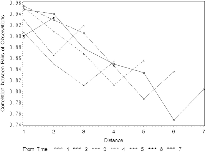
Note that the MODEL statement alone would simply compute ANOVA tables for each hour, as are summarized in Output 8.7. Now we discuss the syntax of the REPEATED statement. Following the key word repeated you see the word HOUR. This is not a variable in the SAS data set FEV1MULT. It is simply a word used to refer to the eight response variables FEV11H, …, FEV18H. This is the basic REPEATED statement. It produces both multivariate and univariate tests that will be discussed later. The PRINTE option at the end of the REPEATED statement produces the sums of squares and cross products of residuals from fitting the model to the eight response variables, and correlation coefficients based on the sum of squares and cross products. The correlation coefficients are shown in Output 8.8.
Output 8.8 Correlations between FEV1 Repeated Measures
| FEV1 Data | |||||||||
| Partial Correlation Coefficients from the Error SS&CP Matrix / Prob > |r| | |||||||||
| DF = 69 | FEV11H | FEV12H | FEV13H | FEV14H | FEV15H | FEV16H | FEV17H | FEV18H | |
| FEV11H | 1.000000 | 0.947354 | 0.939327 | 0.877290 | 0.849003 | 0.833356 | 0.747934 | 0.803328 | |
| 0.0001 | 0.0001 | 0.0001 | 0.0001 | 0.0001 | 0.0001 | 0.0001 | 0.0001 | ||
| FEV12H | 0.947354 | 1.000000 | 0.953603 | 0.928445 | 0.904953 | 0.845329 | 0.786126 | 0.835204 | |
| 0.0001 | 0.0001 | 0.0001 | 0.0001 | 0.0001 | 0.0001 | 0.0001 | 0.0001 | ||
| FEV13H | 0.939327 | 0.953603 | 1.000000 | 0.950646 | 0.907989 | 0.867392 | 0.810935 | 0.855238 | |
| 0.0001 | 0.0001 | 0.0001 | 0.0001 | 0.0001 | 0.0001 | 0.0001 | 0.0001 | ||
| FEV14H | 0.877290 | 0.928445 | 0.950646 | 1.000000 | 0.905495 | 0.848955 | 0.810209 | 0.852875 | |
| 0.0001 | 0.0001 | 0.0001 | 0.0001 | 0.0001 | 0.0001 | 0.0001 | 0.0001 | ||
| FEV15H | 0.849003 | 0.904953 | 0.907989 | 0.905495 | 1.000000 | 0.928608 | 0.864207 | 0.918064 | |
| 0.0001 | 0.0001 | 0.0001 | 0.0001 | 0.0001 | 0.0001 | 0.0001 | 0.0001 | ||
| FEV16H | 0.833356 | 0.845329 | 0.867392 | 0.848955 | 0.928608 | 1.000000 | 0.899701 | 0.932298 | |
| 0.0001 | 0.0001 | 0.0001 | 0.0001 | 0.0001 | 0.0001 | 0.0001 | 0.0001 | ||
| FEV17H | 0.747934 | 0.786126 | 0.810935 | 0.810209 | 0.864207 | 0.899701 | 1.000000 | 0.896999 | |
| 0.0001 | 0.0001 | 0.0001 | 0.0001 | 0.0001 | 0.0001 | 0.0001 | 0.0001 | ||
| FEV18H | 0.803328 | 0.835204 | 0.855238 | 0.852875 | 0.918064 | 0.932298 | 0.896999 | 1.000000 | |
| 0.0001 | 0.0001 | 0.0001 | 0.0001 | 0.0001 | 0.0001 | 0.0001 | 0.0001 | ||
| Applied to Orthogonal Components: |
| Test for Sphericity: Mauchly's Criterion = 0.0654899 |
| Chisquare Approximation = 181.13982 with 27 df Prob > Chisquare = 0.0000 |
The correlation coefficients in Output 8.8, combined with the error mean squares in Output 8.7, tell much about the covariance structure of the data. The correlation between FEV11H and FEV12H through FEV18H generally decrease from 0.95 down to 0.80. Thus, the correlation coefficients generally decrease as length of the time interval increases. This is a common phenomenon of repeated measures. It usually means the covariance structure does not obey the H-F conditions, and, as a consequence, the univariate AVOVA analysis of repeated measures is flawed. Below the correlation coefficients in Output 8.8 you see results of a chi-square test based on the so-called Mauchly’s criterion. This is a likelihood ratio statistic to test whether the model that imposes the H-F conditions on the covariance structure fits as well as the model that imposes no conditions at all. The highly significant chi-square value indicates the H-F conditions are too restrictive. Thus the univariate ANOVA tests in Section 8.2.1 are suspect.
Output 8.9 contains the results of multivariate tests applied to differences between the repeated measures.
Output 8.9 Multivariate Tests for HOUR and DRUG*HOUR Effects
| Manova Test Criteria and Exact F Statistics for the Hypothesis of no HOUR Effect | ||||||
| H = Type III SS&CP Matrix for HOUR E = Error SS&CP Matrix | ||||||
| S=1 M=2.5 N=30.5 | ||||||
| Statistic | Value | F | Num DF | Den DF | Pr > F | |
| Wilks' Lambda | 0.41804056 | 12.5290 | 7 | 63 | 0.0001 | |
| Pillai's Trace | 0.58195944 | 12.5290 | 7 | 63 | 0.0001 | |
| Hotelling-Lawley Trace | 1.39211241 | 12.5290 | 7 | 63 | 0.0001 | |
| Roy's Greatest Root | 1.39211241 | 12.5290 | 7 | 63 | 0.0001 | |
| Manova Test Criteria and F Approximations for the Hypothesis of no HOUR*DRUG Effect | ||||||
| H = Type III SS&CP Matrix for DRUG*HOUR E = Error SS&CP Matrix | ||||||
| S=1 M=2 N=30.5 | ||||||
| Statistic | Value | F | Num DF | Den DF | Pr > F | |
| Wilks' Lambda | 0.51191319 | 3.5789 | 14 | 126 | 0.0001 | |
| Pillai's Trace | 0.55490980 | 3.5108 | 14 | 128 | 0.0001 | |
| Hotelling-Lawley Trace | 0.82292043 | 3.6444 | 14 | 124 | 0.0001 | |
| Roy's Greatest Root | 0.60834527 | 5.5620 | 7 | 64 | 0.0001 | |
| NOTE: F Statistic for Roy's Greatest Root is an upper bound. | ||||||
| NOTE: F Statistic for Wilks' Lambda is exact. | ||||||
| Manova Test Criteria and Exact F Statistics for the Hypothesis of no HOUR*a-c Effect | ||||||
| H = Contrast SS&CP Matrix for HOUR*a-c E = Error SS&CP Matrix | ||||||
| S=1 M=2.5 N=30.5 | ||||||
| Statistic | Value | F | Num DF | Den DF | Pr > F | |
| Wilks' Lambda | 0.81742760 | 2.0101 | 7 | 63 | 0.0676 | |
| Pillai's Trace | 0.18257240 | 2.0101 | 7 | 63 | 0.0676 | |
| Hotelling-Lawley Trace | 0.22334994 | 2.0101 | 7 | 63 | 0.0676 | |
| Roy's Greatest Root | 0.22334994 | 2.0101 | 7 | 63 | 0.0676 | |
The multivariate tests in Output 8.9 show highly significant effects of HOUR and DRUG*HOUR. In this particular example there are highly pronounced changes over time and the changes are not the same for all drugs. Statistical significance of these effects is not really in question. In other examples the trends over time and differences between trends for treatment groups may be less pronounced. In such cases it often happens that the univariate ANOVA tests will indicate statistical significance but the multivariate tests will not. In fact, this phenomenon occurs in the test for interaction between the A-C contrast and HOUR. The univariate ANOVA test in Output 8.6 showed a p-value of 0.0157 for this interaction, but the multivariate test in Output 8.9 shows a p-value of 0.0676. This apparent contradiction might be an artifact of a failed assumption of the H-F covariance structure, leading to a Type I error in the univariate ANOVA. It might also be due to weakness in the multivariate tests because they do not exploit identifiable trends in the covariance structure.
The remaining results from the REPEATED statement are shown in Output 8.10.
Output 8.10 Univariate Tests for DRUG, HOUR and DRUG*HOUR Effects, with Adjusted p-Values
| Tests of Hypotheses for Between Subjects Effects | |||||
| Source | DF | Type III SS | Mean Square | F Value | Pr > F |
| DRUG | 2 | 25.78256701 | 12.89128351 | 3.60 | 0.0327 |
| Error | 69 | 247.41249063 | 3.58568827 | ||
| Univariate Tests of Hypotheses for Within Subject Effects | ||||||
| Source: HOUR | ||||||
| Adj Pr > F | ||||||
| DF | Type III SS | Mean Square | F Value | Pr > F | G - G | H - F |
| 7 | 17.17039931 | 2.45291419 | 38.86 | 0.0001 | 0.0001 | 0.0001 |
| Source: DRUG*HOUR | ||||||
| Adj Pr > F | ||||||
| DF | Type III SS | Mean Square | F Value | Pr > F | G - G | H - F |
| 14 | 6.28006632 | 0.44857617 | 7.11 | 0.0001 | 0.0001 | 0.0001 |
| Source: Error(HOUR) | ||||||
| DF | Type III SS | Mean Square | ||||
| 483 | 30.49025938 | 0.06312683 | ||||
| Greenhouse-Geisser Epsilon = 0.4971 | ||||||
| Huynh-Feldt Epsilon = 0.5419 | ||||||
| Contrast: HOUR*a-b | ||||||
| Adj Pr > F | ||||||
| DF | Type III SS | Mean Square | F Value | Pr > F | G - G | H - F |
| 7 | 1.10406432 | 0.15772347 | 2.50 | 0.0157 | 0.0514 | 0.0461 |
The entries in Output 8.10 duplicate the univariate ANOVA in Output 8.3. The F-test for DRUG in Output 8.10 under the heading “Tests of Hypotheses for between Subject Effects” is the same as that obtained using the TEST option on the RANDOM statement in Output 8.3. The validity of this test does not depend on the covariance structure of repeated measures because it is based on means for each subject averaged over the repeated measures. The tests for HOUR (F = 38.86) and DRUG*HOUR (F = 7.11) in Output 8.3 also are found in Output 8.10 under the heading “Univariate Tests of Hypotheses for Within Subject Effects.” Both of these F-tests show highly significant p-values of 0.0001. The validity of these tests that involve the within-subjects effect HOUR depend on the covariance structure. Specifically, the covariance structure must obey the Huynh-Feldt conditions. In other words, the computed F-values for HOUR and DRUG*HOUR have F-distributions under the respective null hypotheses only if the H-F condition is met. But the results of the chi-square test in Output 8.8 showed that the H-F condition is not met. Thus the univariate ANOVA F-tests are suspect.
Output 8.10 contains two adjusted p-values, labeled G-G and H-F, for the F-tests for HOUR and DRUG*HOUR. These adjustments are obtained by referring the F-values to distributions with reduced degrees of freedom using a method due to Box (1954). The reduced degrees of freedom are equal to the ordinary degrees of freedom multiplied by a number called epsilon. But the value of epsilon depends on unknown parameters and must be estimated. Two estimates of epsilon are given, equal to 0.4971 and 0.5419. The first (G-G) is due to Greenhouse and Geisser (1959) and the second (H-F) is due to Huynh and Feldt (1976). The G-G adjusted p-value for DRUG*HOUR is obtained by referring F = 7.11 to an F-distribution with 14*.4971=6.96 numerator degrees of freedom and 483*.4971=240.1 denominator degrees of freedom. The adjusted p-value is still less than 0.0001. The other adjusted p-values are computed likewise, and all are less than 0.0001. Thus, in this example, the univariate F-values for HOUR and DRUG*HOUR are so large that they are highly significant even with the reduced degrees of freedom. This is not always the case. It commonly happens that the p-value for a univariate F for a within-subjects effect is “significant,” but the adjusted p-value is not. This more or less occurs with interaction contrast A-C*HOUR, for which the univariate ANOVA gave p=.0157, but has G-G and H-F adjusted p-values of 0.0514 and 0.0461, respectively.
8.3.3 Univariate ANOVA of Contrasts of Repeated Measures
The SUMMARY option in the REPEATED statement provides univariate ANOVA results of contrast variables. Results appear in Output 8.11.
Output 8.11 Univariate Tests for Contrast Variables
| Analysis of Variance of Contrast Variables | |||||
| HOUR.N represents the contrast between the nth level of HOUR and the last | |||||
| Contrast Variable: HOUR.1 | |||||
| Source | DF | Type III SS | Mean Square | F Value | Pr > F |
| MEAN | 1 | 15.47533889 | 15.47533889 | 81.76 | 0.0001 |
| DRUG | 2 | 4.95388611 | 2.47694306 | 13.09 | 0.0001 |
| Error | 69 | 13.05957500 | 0.18926920 | ||
| Contrast | DF | Contrast SS | Mean Square | F Value | Pr > F |
| a-c | 1 | 0.05135208 | 0.05135208 | 0.27 | 0.6041 |
| Contrast Variable: HOUR.2 | |||||
| Source | DF | Type III SS | Mean Square | F Value | Pr > F |
| MEAN | 1 | 13.84256806 | 13.84256806 | 82.37 | 0.0001 |
| DRUG | 2 | 2.85541111 | 1.42770556 | 8.50 | 0.0005 |
| Error | 69 | 11.59632083 | 0.16806262 | ||
| Contrast | DF | Contrast SS | Mean Square | F Value | Pr > F |
| a-c | 1 | 0.07207500 | 0.07207500 | 0.43 | 0.5147 |
| Contrast Variable: HOUR.3 | |||||
| Source | DF | Type III SS | Mean Square | F Value | Pr > F |
| MEAN | 1 | 8.96761250 | 8.96761250 | 62.21 | 0.0001 |
| DRUG | 2 | 1.95842500 | 0.97921250 | 6.79 | 0.0020 |
| Error | 69 | 9.94626250 | 0.14414873 | ||
| Contrast | DF | Contrast SS | Mean Square | F Value | Pr > F |
| a-c | 1 | 0.69841875 | 0.69841875 | 4.85 | 0.0311 |
| FEV1 Data | |||||
| Contrast Variable: HOUR.4 | |||||
| Source | DF | Type III SS | Mean Square | F Value | Pr > F |
| MEAN | 1 | 4.63093889 | 4.63093889 | 31.57 | 0.0001 |
| DRUG | 2 | 1.19181111 | 0.59590556 | 4.06 | 0.0215 |
| Error | 69 | 10.12265000 | 0.14670507 | ||
| Contrast | DF | Contrast SS | Mean Square | F Value | Pr > F |
| a-c | 1 | 0.72030000 | 0.72030000 | 4.91 | 0.0300 |
| Contrast Variable: HOUR.5 | |||||
| Source | DF | Type III SS | Mean Square | F Value | Pr > F |
| MEAN | 1 | 1.77347222 | 1.77347222 | 19.50 | 0.0001 |
| DRUG | 2 | 0.54738611 | 0.27369306 | 3.01 | 0.0559 |
| Error | 69 | 6.27594167 | 0.09095568 | ||
| Contrast | DF | Contrast SS | Mean Square | F Value | Pr > F |
| a-c | 1 | 0.02296875 | 0.02296875 | 0.25 | 0.6169 |
| Contrast Variable: HOUR.6 | |||||
| Source | DF | Type III SS | Mean Square | F Value | Pr > F |
| MEAN | 1 | 0.62533472 | 0.62533472 | 9.28 | 0.0033 |
| DRUG | 2 | 0.02916944 | 0.01458472 | 0.22 | 0.8058 |
| Error | 69 | 4.64719583 | 0.06735066 | ||
| Contrast | DF | Contrast SS | Mean Square | F Value | Pr > F |
| a-c | 1 | 0.02566875 | 0.02566875 | 0.38 | 0.5390 |
| FEV1 Data | |||||
| Contrast Variable: HOUR.7 | |||||
| Source | DF | Type III SS | Mean Square | F Value | Pr > F |
| MEAN | 1 | 0.00700139 | 0.00700139 | 0.07 | 0.7953 |
| DRUG | 2 | 0.08841944 | 0.04420972 | 0.43 | 0.6535 |
| Error | 69 | 7.12547917 | 0.10326781 | ||
| Contrast | DF | Contrast SS | Mean Square | F Value | Pr > F |
| a-c | 1 | 0.02296875 | 0.02296875 | 0.22 | 0.6387 |
The contrasts are differences between each hour and hour 8. For example, HOUR.1 is the difference between hour 1 and hour 8. For each contrast variable there are tests labeled MEAN, DRUG, and A-C. These results are what you would obtain if you created the differences in a SAS data set and ran univariate analyses on the contrasts. Since they are univariate analyses, their validity does not depend on the covariance structure. See Littell et al. (1998) for more details.
Some care is required to correctly interpret the tests in Output 8.11. Consider the variable HOUR.1. The F-test for DRUG is highly significant with p<0.0001. This is evidence that the means of the variable HOUR.1 for the three drugs are different. But since the variable HOUR.1 is the difference between hours 1 and 8, the test for DRUG is really a test of whether the change from hour 1 to hour 8 differs between the drugs. Thus the test for DRUG is really a test for the interaction between drugs and the contrast hour 1 minus hour 8. Likewise, the test for A-C is a test for the interaction between the drug contrast A-C and the hour contrast 1-8. The test for MEAN is a test of whether the average value of HOUR.1 over the drugs differs from zero.
8.4 Mixed-Model Analysis of Repeated Measures
The first sections of this chapter reviewed methods for repeated-measures data that predate the availability of PROC MIXED. Data analysts essentially faced a choice between “split-plot in time” univariate ANOVA, presented in Section 8.2, contrasts, or multivariate analysis of variance (MANOVA), as presented in Section 8.3. These approaches all have serious drawbacks.
As noted earlier in this chapter, univariate ANOVA assumes that within-subjects errors are uncorrelated, or, equivalently, that correlation between observations on the same subject is constant, regardless of the time lapse between pairs of observations. This is often an unrealistic assumption. If you ignore time-dependent correlation, you risk underestimating standard errors of mean comparisons involving different times and overestimating test statistics for time and time-by-treatment effects, resulting in excessive Type I error rates. While adjustments such as the Greenhouse-Geisser and Huynh-Feldt corrections used in PROC GLM attempt to account for within-subjects correlation, these corrections are often inadequate and, in any event, do not address the impact of correlation on standard errors of differences that may be of interest to researchers.
MANOVA assumes a correlation structure that is far more general than most repeated-measures data require. The MANOVA covariance matrix assumes that the correlation between every pair of times of observation within subjects is unique. For example, the correlations between the first and second, second and third, third and fourth, and so on, observations are each unique parameters in MANOVA. Usually, a simpler model, such as a single correlation parameter for all observations that are adjacent in time, is sufficient to characterize the data. Thus, MANOVA typically wastes a great deal of information, which in turn adversely affects efficiency and power. Moreover, if an observation is lost at a single time for a given subject, MANOVA must delete the entire subject. Thus, a great deal of valid data may be thrown out, a draconian approach to missing data.
The mixed-model procedures of PROC MIXED allow a flexible approach to modeling correlated errors. By using a parsimonious covariance model that adequately accounts for within-subjects correlation, you can avoid the problems associated with univariate and multivariate ANOVA.
As noted in the introduction to this chapter, mixed-model analysis involves two stages: first, estimate the covariance structure, then second, assess treatment and time effects using generalized least squares with the estimated covariance. Littell, Pendergast, and Natajan (2000) break these stages further into a four-step procedure for mixed-model analysis:
Step 1: Model the mean structure, usually by specification of the fixed effects.
Step 2: Specify the covariance structure, between subjects as well as within subjects.
Step 3: Fit the mean model accounting for the covariance structure; MIXED uses generalized least squares to do this.
Step 4: Make statistical inference based on the results of Step 3; this step may include making the means model more parsimonious.
As Littell et al. (2000) point out, other authors, for example, Diggle (1988) and Wolfinger (1993), recommend similar model-fitting and inference processes. The following sections show you how to use PROC MIXED to implement these fours steps. Sections 8.4.1 through 8.4.4 apply Steps 1 through 4, respectively, to the univariate data (FEV1UNI) from Output 8.2.
8.4.1 The Fixed-Effects Model and Related Considerations
The model equation for mixed-model analysis is identical to the univariate ANOVA model described in Section 8.2. Model (8.2) is a mixed model for the FEV1 data.
As discussed earlier, the FEV1 data set contains a baseline observation, BASEFEV1, on each subject. Often, you can get a more accurate assessment of treatment effects by accounting for baseline measurements in the model using analysis of covariance. A model accounting for baseline observations is
yijk = μ + αi + βXij + bij + γk + (αγ)ik + eijk (8.3)
where Xij is the baseline observation on the ijth subject, β is the regression coefficient, and all other terms are as defined previously for model (8.2).
The analyses presented in Sections 8.2 and 8.3 do not lend themselves to using baseline data. In general, for any data with repeated measures or split-plot features, analysis of covariance with covariates observed on the larger units—for example, subjects or whole-plot experimental units—is difficult and awkward, if not impossible, to implement with PROC GLM, or any other procedure not explicitly written to use mixed-model methods. However, baseline covariate models are relatively easy to compute with PROC MIXED.
In the mixed model, the between-subjects error, bij and the within-subjects error, eijk, are considered random effects. The bij’s and eijk’s are assumed to be independent of one another. For each set of effects, the covariance structure can be quite general.
Typically, the between-subjects errors are assumed i.i.d. N(0, ). Thus, the vector of random model effects, b′ = ~ MVN(0,I). The covariance for the within-subjects effects is more complex. Denote e′ij as the vector of within-subjects errors for the ijth subject. In general, eij ~ MVN(0,Σ), where Σ is a K×K covariance matrix. The full vector of within-subjects errors, e′= is distributed MVN(0,R), where R is a block diagonal matrix, with one block per subject, and each block equal to Σ. Thus R= where is the total number of subjects.
PROC MIXED allows you to choose from many covariance models, in other words, forms of Σ. The simplest model is the independent covariance model, where the within-subjects error correlation is zero, and hence Σ=IσS2. The most complex is the unstructured covariance model, where within-subjects errors for each pair of times have their own unique correlation, and hence . In some applications, the within-subjects correlation is negligible. For example, in some agronomic and large animal nutrition trials, repeated measurements may occur at long enough intervals, for example, monthly, so that correlation is effectively zero relative to other variation. In such cases, the independent structure is acceptable. However, this should be checked before analyzing the data assuming uncorrelated errors.
In most experiments, some correlation is present. However, correlation is usually not as complex as the unstructured model. The simplest correlation model is compound symmetry, referred to as CS in PROC MIXED syntax. The CS model is written
It assumes that correlation is constant regardless of the distance between pairs of repeated measurements. Note that the split-plot model, yijk = μ + αi + bij + γk + (αγ)ik + eijk, with independent errors, and the model yijk = μ + αi + γk + (αγ)ik + eijk, dropping bij and assuming compound symmetry among the eijk for the ijth subject, are equivalent expressions of the same model. Under the independent errors model, var(yijk)= and cov(yijk ,yijk) = for k≠k′, identical to the CS model with and and .
Typically, correlation between observations is a function of their distance in time: adjacent observations tend to be more highly correlated than observations farther apart in time. Several models may adequately describe such correlation. The simplest is the first-order autoregressive, or AR(1), model. For the AR(1),
The AR(1) model assumes that where where sijk ~N(0,). It follows that . It follows that . This helps explain why independent errors models tend to underestimate within-subjects variance when correlation among the errors is non-negligible.
For AR(1), correlation between adjacent within-subjects errors is ρ, regardless of whether the pair of observations is the 1st and 2nd, 2nd and 3rd, or (K–1)st and Kth. With the unstructured model, each pair has its own correlation. The correlation is ρ2 for any pair of errors 2 units apart, for example, the 1st and 3rd. In general, errors d units apart have correlation ρd. Note that the AR(1) model requires estimates of just two parameters, σ2 and ρ, whereas unstructured models require estimating parameters.
The Toeplitz model is similar to the AR(1) model in the sense that pairs of within-subjects errors separated by a common distance share the same correlation. Errors d units apart have correlation ρd. However, there is no known function relating ρd to d. Thus, for the Toeplitz model,
The Toeplitz model is less restrictive than AR(1), but it requires estimating K parameters (σ2, ρ1,...,ρK-1) instead of just two.
The AR(1) and Toeplitz models make sense when observations are equally spaced and the correlation structure does not change appreciably over time. A more general model that preserves the main features of these models, but allows for unequal spacing and change over time is the first-order ante dependence model, or ANTE(1). The model structure is
You can see that the ANTE(1) model permits the variance among observations to change over time. Correlation between pairs of observations is the product of the correlations between adjacent times between observations, so that correlation may change over time. The ANTE(1) model requires estimating 2K–1 parameters.
There are several other structures, including the first-order autoregressive model and Toeplitz models that allow for unequal variances over time, ARH(1) and TOEPH, respectively. See SAS OnlineDoc,Version 8 for a complete listing of the covariance structures available in PROC MIXED.
Section 8.4.2 presents methods for selecting an appropriate covariance model—that is, a model that adequately accounts for within-subjects correlation but does not require estimating an excessive number of covariance parameters. As with any model selection activity, evaluating covariance structure should not be a purely statistical exercise. You should first rule out covariance structures that clearly make no sense in the context of a given data set. For example, AR(1) or TOEP models are generally inappropriate if the times of observation are not equally spaced either chronologically or in terms of some meaningful criterion such as biological stage of development.
8.4.2 Selecting an Appropriate Covariance Model
To draw accurate conclusions from repeated-measures data, you must use an appropriate model of within-subjects correlation. If you ignore important correlation by using a model that is too simple, you risk increasing Type I error rate and underestimating standard errors. If the model is too complex you sacrifice power and efficiency. Guerin and Stroup (2000) documented the effects of various covariance modeling decisions using PROC MIXED for repeated-measures data. Their work supports the idea that repeated-measures analysis is robust as long as the covariance model used is approximately correct, but inference is severely compromised by blatantly poor choice of a covariance model. This is the philosophy underlying this section.
This section illustrates two types of tools you can use with PROC MIXED to help you select a covariance model. First are graphical tools to help visualize patterns of correlation between observations at different times. Second are information criteria that measure the relative fit of competing covariance models. As noted at the end of the last section, these methods work best when you first rule out covariance structures that are obviously inconsistent with the characteristics of the data you are analyzing.
You can visualize the correlation structure by plotting changes in covariance and correlation among residuals on the same subject at different times over distance between times of observation. Distance between times is called lag. Although you can use either PROC GLM or PROC MIXED to create the data sets needed for these plots, PROC MIXED is easier. To see why, consider PROC GLM first. With PROC GLM, you can use using the following SAS statements to obtain residuals from the multivariate form of the data given in Output 8.1:
proc glm data=fev1mult;
class drug;
model fev11h fev12h fev13h fev14h fev15h fev16h
fev17h fev18h=drug;
output out=resid residual=e1-e8;
This program outputs the residuals from the means model. The variable E1 denotes residuals at time 1, E2 at time 2, and so forth. You can use the output data set RESID to construct scatter plots among the residuals for all pairs of times, as shown by Littell et al. (2000). Once you compute the residuals, you can use PROC CORR to compute correlation and the sum of squares and cross-products among the residuals for all pairs of times. Although PROC CORR has an option to compute covariance, for repeated measures it is unable to determine the correct denominator degrees of freedom, so the covariance is computed incorrectly.
You can obtain correlation and covariance among residuals more simply and in more readily usable form for plotting with the following PROC MIXED statements:
proc mixed data=fev1uni;
class drug patient hour;
model fev1=drug|hour;
repeated /type=un subject=patient(drug) sscp rcorr;
ods output covparms=cov;
ods output rcorr=corr;
Note that PROC MIXED uses the univariate form of the FEV1 data. The MODEL follows from the fixed-effects of model (8.2) given in Section 8.2. The REPEATED statement determines the form of the covariance among the eijk . TYPE=UN specifies an unstructured correlation model, as described in Section 8.4.1. SUBJECT=PATIENT(DRUG) specifies that errors are correlated within each PATIENT(DRUG)—that is, observations on different PATIENT(DRUG) levels are independent, but observations on the same PATIENT(DRUG) are not. In mixed-model covariance matrix terms, TYPE= specifies the form of Σ and SUBJECT= specifies the block in the block diagonal structure of R, that is, R= . The SSCP option causes the σkk′ = cov(eijk’, eijk’) to be computed directly from the corrected sums of squares and cross products matrix rather than the default REML procedure. The RCORR option causes the correlations to be computed as well as the covariance matrix. The two ODS statements create new SAS data sets containing the covariances and correlations, respectively.
Use the following SAS statements to create the first plot for visualizing an appropriate covariance model:
data times;
do time1=1 to 8;
do time2=1 to time1;
dist=time1-time2;
output;
end;
end;
data covplot;
merge times cov;
proc print;
axis1 value=(font=swiss2 h=2) label=(angle=90 f=swiss
h=2 'Covariance of Between Subj Effects'),
axis2 value=(font=swiss h=2) label=(f=swiss h=2 'Distance'),
legend1 value=(font=swiss h=2) label=(f=swiss h=2 'From Time'),
symbol1 color=black interpol=join
line=1 value=square;
symbol2 color=black interpol=join
line=2 value=circle;
symbol3 color=black interpol=join
line=20 value=triangle;
symbol4 color=black interpol=join
line=3 value=plus;
symbol5 color=black interpol=join
line=4 value=star;
symbol6 color=black interpol=join
line=5 value=dot;
symbol7 color=black interpol=join
line=6 value=_;
symbol8 color=black interpol=join
line=10 value==;
proc gplot data=covplot;
plot estimate*dist=time2/vaxis=axis1 haxis=axis2
legend=legend1;
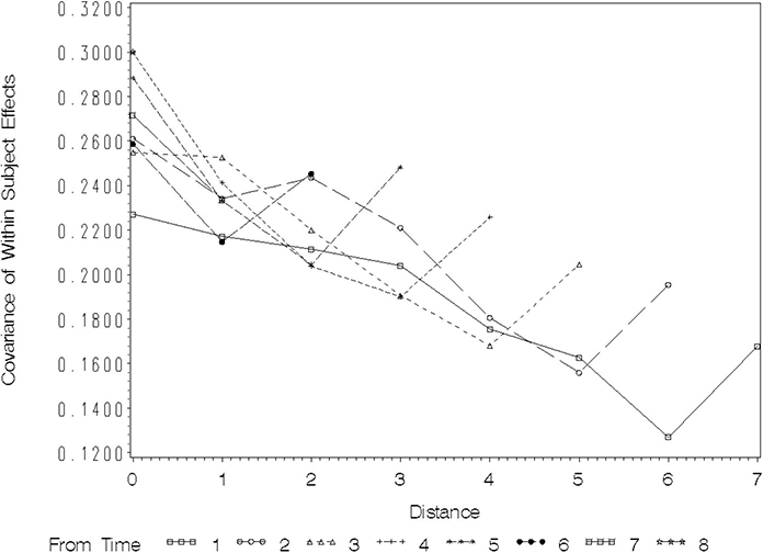
First, you create a data set called TIMES containing the pairs of observation times and the distance between them. You then merge the data set TIMES with the covariance data set COV created by the first ODS statement in the PROC MIXED program given above. The resulting data set COVPARMS appears in Output 8.12. The GPLOT procedure with its associated AXIS, LEGEND, and SYMBOL definitions creates a plot of covariance between pairs of repeated measures by distance, shown in Figure 8.2.
Output 8.12 Data Set Containing Pairs of Times and Estimates
| Obs | time1 | time2 | dist | CovParm | Subject | Estimate | adjcov | adjcorr |
| 1 | 1 | 1 | 0 | UN(1,1) | PATIENT(DRUG) | 0.4541 | 0.08893 | 0.24350 |
| 2 | 2 | 1 | 1 | UN(2,1) | PATIENT(DRUG) | 0.4587 | 0.09352 | 0.25607 |
| 3 | 2 | 2 | 0 | UN(2,2) | PATIENT(DRUG) | 0.5163 | 0.15108 | 0.41370 |
| 4 | 3 | 1 | 2 | UN(3,1) | PATIENT(DRUG) | 0.4441 | 0.07894 | 0.21617 |
| 5 | 3 | 2 | 1 | UN(3,2) | PATIENT(DRUG) | 0.4808 | 0.11556 | 0.31644 |
| 6 | 3 | 3 | 0 | UN(3,3) | PATIENT(DRUG) | 0.4923 | 0.12711 | 0.34806 |
| 7 | 4 | 1 | 3 | UN(4,1) | PATIENT(DRUG) | 0.4154 | 0.05023 | 0.13754 |
| 8 | 4 | 2 | 2 | UN(4,2) | PATIENT(DRUG) | 0.4688 | 0.10358 | 0.28362 |
| 9 | 4 | 3 | 1 | UN(4,3) | PATIENT(DRUG) | 0.4687 | 0.10351 | 0.28344 |
| 10 | 4 | 4 | 0 | UN(4,4) | PATIENT(DRUG) | 0.4938 | 0.12858 | 0.35208 |
| 11 | 5 | 1 | 4 | UN(5,1) | PATIENT(DRUG) | 0.4349 | 0.06974 | 0.19098 |
| 12 | 5 | 2 | 3 | UN(5,2) | PATIENT(DRUG) | 0.4943 | 0.12912 | 0.35355 |
| 13 | 5 | 3 | 2 | UN(5,3) | PATIENT(DRUG) | 0.4843 | 0.11912 | 0.32619 |
| 14 | 5 | 4 | 1 | UN(5,4) | PATIENT(DRUG) | 0.4837 | 0.11851 | 0.32452 |
| 15 | 5 | 5 | 0 | UN(5,5) | PATIENT(DRUG) | 0.5779 | 0.21273 | 0.58249 |
| 16 | 6 | 1 | 5 | UN(6,1) | PATIENT(DRUG) | 0.3934 | 0.02816 | 0.07711 |
| 17 | 6 | 2 | 4 | UN(6,2) | PATIENT(DRUG) | 0.4254 | 0.06024 | 0.16496 |
| 18 | 6 | 3 | 3 | UN(6,3) | PATIENT(DRUG) | 0.4263 | 0.06109 | 0.16728 |
| 19 | 6 | 4 | 2 | UN(6,4) | PATIENT(DRUG) | 0.4179 | 0.05265 | 0.14418 |
| 20 | 6 | 5 | 1 | UN(6,5) | PATIENT(DRUG) | 0.4945 | 0.12927 | 0.35397 |
| 21 | 6 | 6 | 0 | UN(6,6) | PATIENT(DRUG) | 0.4906 | 0.12542 | 0.34343 |
| 22 | 7 | 1 | 6 | UN(7,1) | PATIENT(DRUG) | 0.3562 | -0.00901 | -0.02467 |
| 23 | 7 | 2 | 5 | UN(7,2) | PATIENT(DRUG) | 0.3992 | 0.03398 | 0.09305 |
| 24 | 7 | 3 | 4 | UN(7,3) | PATIENT(DRUG) | 0.4021 | 0.03690 | 0.10105 |
| 25 | 7 | 4 | 3 | UN(7,4) | PATIENT(DRUG) | 0.4023 | 0.03714 | 0.10171 |
| 26 | 7 | 5 | 2 | UN(7,5) | PATIENT(DRUG) | 0.4643 | 0.09909 | 0.27133 |
| 27 | 7 | 6 | 1 | UN(7,6) | PATIENT(DRUG) | 0.4454 | 0.08015 | 0.21948 |
| 28 | 7 | 7 | 0 | UN(7,7) | PATIENT(DRUG) | 0.4994 | 0.13422 | 0.36753 |
| 29 | 8 | 1 | 7 | UN(8,1) | PATIENT(DRUG) | 0.3840 | 0.01878 | 0.05143 |
| 30 | 8 | 2 | 6 | UN(8,2) | PATIENT(DRUG) | 0.4257 | 0.06046 | 0.16557 |
| 31 | 8 | 3 | 5 | UN(8,3) | PATIENT(DRUG) | 0.4256 | 0.06044 | 0.16549 |
| 32 | 8 | 4 | 4 | UN(8,4) | PATIENT(DRUG) | 0.4251 | 0.05989 | 0.16400 |
| 33 | 8 | 5 | 3 | UN(8,5) | PATIENT(DRUG) | 0.4950 | 0.12984 | 0.35553 |
| 34 | 8 | 6 | 2 | UN(8,6) | PATIENT(DRUG) | 0.4632 | 0.09799 | 0.26832 |
| 35 | 8 | 7 | 1 | UN(8,7) | PATIENT(DRUG) | 0.4496 | 0.08443 | 0.23119 |
| 36 | 8 | 8 | 0 | UN(8,8) | PATIENT(DRUG) | 0.5031 | 0.13791 | 0.37763 |
You can see that data set COVPLOT contains the time pairs and distance between them created in the data set TIMES and the covariance information created in the ODS step of PROC MIXED. Notice that because of the way the ODS statement constructs the data set COV, the variable TIME2 is actually the observation in the pair that is taken first. In the plot shown in Figure 8.2, notice that there are seven profiles, each corresponding to the time of the first observation in the pair. Since the variable TIME2 is the first observation in the pair, this explains why you use TIME2 in the PLOT statement of PROC GPLOT.
Figure 8.2 Plot of Covariance as a Function of Distance in Time between Pairs of Observations
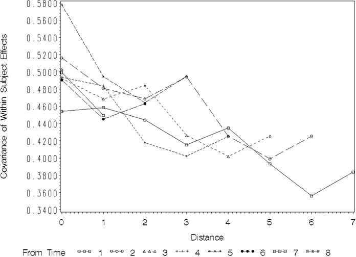
The values plotted at distance=0 are the variances among the observations at each of the eight times. These range from roughly 0.45 to just less than 0.60. This, and the fact that there is no trend of increasing or decreasing variance with time of observation, suggests that a covariance model with constant variance over time is probably adequate. You will see how to confirm this more formally when we discuss model-fitting criteria below.
Figure 8.2 shows that for the FEV1 data, as the distance between pairs of observations increases, covariance tends to decrease. Also, the pattern of decreasing covariance with distance is roughly the same for all reference times, although seeing this takes a bit of practice. Start with the profile labeled “From Time 1,” which gives the HOUR of the first observation of a given pair of repeated measures. The square symbol on the plot tracks the covariance between pairs of repeated measurements whose first observation occurs at HOUR=1. The position of this plot at distance 0 plots the sample variance of observations taken at hour 1. The plot at distance 1 gives the covariance between hours 1 and 2, distance 2 plots covariance for hours 1 and 3, and so forth. Following the profile across the distances shows how the covariance decreases as distance increases for pairs of observations whose first time of observation is HOUR=1. You can see that there is a general pattern of decrease from roughly 0.50 at distance 1 to a little less than 0.40. If you follow the plots labeled “From Time” 2, 3, and so forth, the overall pattern is very similar. The covariance among adjacent observations is consistently between 0.45 and 0.50, with the HOUR of the first element of the pair making little difference. The covariance at distance 2 is a bit lower, averaging around 0.45, and does not appear to depend on the hour of the first element of the pair.
You can draw two main conclusions from this plot:
1. AR(1) or Toeplitz covariance models are probably most appropriate for the data. They allow covariance to decrease with increasing distance and they assume that correlation is strictly a function of distance and does not depend on the time of the first observation in the pair. Compound symmetry appears to be inappropriate because the covariance does not remain constant for all distances; unstructured, ante dependence, or heterogeneous variance models also are probably inappropriate because there is no visual evidence of changes in variance or covariance-distance relationships over time.
2. The between-subjects variance component, σB 2 is nonzero. In fact, it is roughly between 0.35 and 0.40. Note that all of the plots of covariance decline for distances 1, 2, and 3, and then seem to flatten out. This is exactly what should happen if the between-subjects variance component is approximately equal to the plotted covariance at the larger distances and there is AR(1) correlation among the observations within each subject. At the larger distances the AR(1) correlation ρd, should approach zero. The nonzero covariance plotted for larger distances results from the intraclass correlation .
Figure 8.3 shows idealized plots for three covariance structures: compound symmetry, AR(1) only, and AR(1)+random between-subjects effects.
Figure 8.3 Idealized Plot of Covariance by Distance for Three Covariance Models
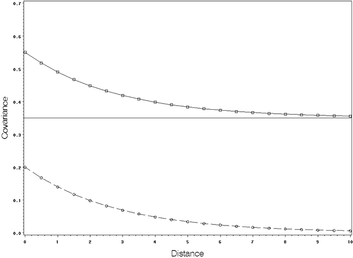
The flat line across all distances at an approximate covariance of 0.35 shows the plot you would expect to see with compound symmetry. The plot with a covariance decreasing from approximately 0.20 to 0 as distance increases is what you would expect to see with pure AR(1) covariance. The plot that decreases from approximately 0.55 to 0.35 is the expected plot from the AR(1)+random between-subjects effects model. The numbers on the covariance axis follow from the approximate magnitudes of the observed covariances in Output 8.12 and Figure 8.2. You can see that the plots of observed covariances in Figure 8.2 correspond most closely to the AR(1)+random between-subjects effects model.
You can remove the between-subjects component and plot the remaining within-subjects covariance. Use the SAS statements
data covplot;
merge times cov;
adjcov=estimate-0.3652;
adjcorr=adjcov/0.3652;
Note that these statements simply add the ADJCOV and ADJCORR formula to the statements used previously to create the COVPLOT data set. You use the minimum covariance among pairs of repeated measures—specifically , UN(7,1) in Output 8.12. This is a reasonable lower bound on B 2 from the covariance plot. ADJCOV simply removes B 2 from the covariance. ADJCORR assumes that an upper bound of the correlation between a pair of repeated measures, . ADJCOV and ADJCORR appear in Output 8.12. You can revise the PROC GPLOT statements used to create Figure 8.2 to plot these values by distance. Figure 8.4 shows the adjusted correlation. The adjusted covariance is not shown.
Figure 8.4 Plot of Approximate Adjusted Correlation by Distance
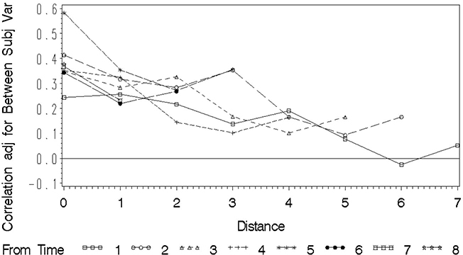
These plots reveal essentially the same pattern as in Figure 8.2. The values at distance 0 for ADJCORR in Output 8.15 are meaningless. Starting with distance 1, the correlation is between 0.44 and 0.50 and decreases to essentially zero by distance 6. Again, these values seem consistent with either the AR(1) or Toeplitz model. Because AR(1) requires fewer parameters, it is the more parsimonious model and thus it may be the better choice.
You can also plot the unadjusted correlation by distance using the data set CORR created by the second ODS statement in the PROC MIXED program at the beginning of this section. The form of the data set is not as convenient, but the following statements allow you to create the plot, which appears in Figure 8.5. The AXIS2, LEGEND, and SYMBOL statements for the PROC GPLOT statements are identical to those used for Figure 8.2. Only the AXIS1 LABEL is changed.
data corrlplot;
set corr;
if row=1 then do;
dist=1; corr=col2; output;
dist=2; corr=col3; output;
dist=3; corr=col4; output;
dist=4; corr=col5; output;
dist=5; corr=col6; output;
dist=6; corr=col7; output;
dist=7; corr=col8; output;
end;
if row=2 then do;
dist=1; corr=col3; output;
dist=2; corr=col4; output;
dist=3; corr=col5; output;
dist=4; corr=col6; output;
dist=5; corr=col7; output;
dist=6; corr=col8; output;
end;
if row=3 then do;
dist=1; corr=col4; output;
dist=2; corr=col5; output;
dist=3; corr=col6; output;
dist=4; corr=col7; output;
dist=5; corr=col8; output;
end;
if row=4 then do;
dist=1; corr=col5; output;
dist=2; corr=col6; output;
dist=3; corr=col7; output;
dist=4; corr=col8; output;
end;
if row=5 then do;
dist=1; corr=col6; output;
dist=2; corr=col7; output;
dist=3; corr=col8; output;
end;
if row=6 then do; output;
dist=1; corr=col7; output;
dist=2; corr=col8; output;
end;
if row=7 then do;
dist=1; corr=col8; output;
end;
axis1 value=(font=swiss2 h=2) label=(angle=90 f=swiss
h=2 'Correlation between Pairs of Observations'),
proc gplot data=corrlplot;
plot corr*dist=row/vaxis=axis1 haxis=axis2
legend=legend1;
You can see from Figure 8.5 that correlation decreases from roughly 0.90-0.95 at distance 1 to approximately 0.80 for a pair of observations whose distance exceeds 5 units in time. From Output 8.12, the adjusted variance after removing σB2 was between 0.15 and 0.20. This provides a crude idea of what you can expect the within-subjects variance σS 2 to be. The intraclass correlation could then be very crudely approximated by . This is fairly close to the value approached by the correlation at larger distances in the plot in Figure 8.4. As with the covariance plot of Figure 8.2, when the correlation plot appears to asymptotically approach a value appreciably greater than 0 for the larger distances, this suggests a correlation process among the repeated measures over and above a substantial between-subjects error component. A flat correlation plot over distance would suggest compound symmetry. Here, the plot is not flat for the shorter distances, suggesting a within-subjects correlation model for which correlation is a decreasing function of distance. This is very similar to the conclusion you can draw from the covariance plots discussed earlier. One disadvantage of the correlation plot is that at distance 0, correlation always equals 1 regardless of the variance. This means you cannot use the correlation plot to diagnose possible heterogeneous variance over time, as you can with the covariance plots.
Figure 8.5 Plot of Correlation between Repeated Measurements by Distance between Times of Observation
8.4.3 Reassessing the Covariance Structure with a Means Model Accounting for Baseline Measurement
Recall at the beginning of Section 8.4.1 we discussed the possible use of the baseline covariate BASEFEV1. You can refit the means model to include the covariate, output the resulting covariance and correlation matrices, and plot them using the same approach used for Figures 8.2, 8.4, and 8.5. The revised PROC MIXED statements for the baseline covariate model are
proc mixed data=fev1uni;
class drug hour patient;
model fev1=drug|hour basefev1;
repeated / type=un sscp subject=patient(drug) rcorr;
ods output covparms=cov;
ods output rcorr=corr;
Figure 8.6 shows the plot of the covariance by distance.
Figure 8.6 Plot of Covariance as a Function of Distance in Time between Pairs of Observations
The pattern of Figure 8.6 is similar to Figure 8.2 except that using BASEFEV1 as a covariate substantially reduces the variance—from roughly 0.50 to less than 0.30. As distance increases, the covariance appears to reach an asymptote between 0.15 and 0.20. Again, this suggests a between-subjects variance between 0.15 and 0.20, and an additional within-subjects covariance model with covariance a decreasing function of distance, but independent of time.
8.4.4 Information Criteria to Compare Covariance Models
The default output from PROC MIXED includes values under the heading “Fit Statistics.” These include –2 × the Residual (or REML) Log Likelihood (labeled “–2 Res Log Likelihood”), and three information criteria. In theory, the greater the residual log likelihood, the better the fit of the model. However, somewhat analogously to R2 in multiple regression, you can always improve the log likelihood by adding parameters to the point of absurdity.
Information criteria attach penalties to the log likelihood. The information criterion equals the residual log likelihood minus some function of the number of parameters in the covariance model, or, alternatively, –2 × the residual log likelihood plus –2 × the function of the number of covariance model parameters. The latter form is used beginning with Release 8.2 of PROC MIXED. For example, the penalty for the compound symmetry model is a function of 2, because there are two covariance parameters, ʵ2 and ρ. The penalty for an unstructured model is a function of . Hence, the residual log likelihood for an unstructured model is always greater than the residual log likelihood for compound symmetry, but the penalty is always greater as well. Unless the improvement in the residual log likelihood exceeds the size of the penalty, the simpler model yields the higher information criterion and is thus the preferred covariance model.
Two commonly used information criteria are Akaike’s (1974) and Schwarz’s (1978). A more recent information criterion, also included as a default starting with Release 8.2 of PROC MIXED, is a finite-population corrected Akaike criterion developed by Burnham and Anderson (1998). The Akaike Information Criterion is often referred to by the acronym AIC. The finite-population corrected AIC has the acronym AICC. Two commonly used acronyms for Schwarz’s Bayesian Information Criterion are BIC and SBC—hereafter this text uses the latter. Refer to SAS OnlineDoc, Version 8 for a complete explanation of how these terms are computed.
The basic idea for repeated-measures analysis is that among the models for within-subjects covariance that are considered plausible in the context of a particular study (for example, biologically or physically reasonable), the model that minimizes the AIC, AICC, or SBC—in its –2 × (REML log likelihood penalty) form—is the preferred model. When AIC, AICC, or SBC are close, the simpler model is generally considered preferable in the interest of using a parsimonious model.
Keselman et al. (1998) compared AIC and SBC for their ability to select “the right” covariance model. Their study used Release 6.12 of SAS, which was determined to compute SBC incorrectly. This was corrected in Release 8.0. Guerin and Stroup (2000) compared the information criteria using Release 8.0 for their ability to select “the right” model and for the impact of choosing “the wrong” model on Type I error rate. They found that AIC tends to choose more complex models than SBC. They found that choosing a model that is too simple affects Type I error control more adversely than choosing a model that is too complex. When Type I error control is the highest priority, AIC is the model-fit criterion of choice. However, if loss of power is relatively more serious, SBC may be preferable. AICC was not available at the time of the Guerin and Stroup study; a reasonable inference from their study is that its performance is similar to AIC, but somewhat less likely to choose a more complex model. Thus, loss of power is less than with AIC, but still greater than with SBC.
You can compare candidate covariance models by running PROC MIXED with the same fixed-effects model, varying the RANDOM and REPEATED statements to obtain the AIC, AICC, and SBC for all candidate models. For the FEV1 data, the models that appear to warrant consideration based on the covariance plots are the AR(1) and the Toeplitz models, both in conjunction with a between-subjects random effect. For the AR(1) model, the needed SAS statements are
proc mixed;
class drug hour patient;
model fev1=drug|hour basefev1;
random patient(drug);
repeated / type=ar(1) subject=patient(drug);
The parameter estimates and fit statistics appear in Output 8.13.
Output 8.13 Covariance Parameter Estimates and Fit Statistics for FEV1 Data Using the AR(1) Model
| Covariance Parameter Estimates | ||
| Cov Parm | Subject | Estimate |
| PATIENT(DRUG) | 0.1848 | |
| AR(1) | PATIENT(DRUG) | 0.5401 |
| Residual | 0.08309 | |
| Fit Statistics | |
| -2 Res Log Likelihood | 247.0 |
| AIC (smaller is better) | 253.0 |
| AICC (smaller is better) | 253.1 |
| BIC (smaller is better) | 259.9 |
Note the close correspondence between the REML estimates of between-subjects variance (the PATIENT(DRUG) variance, 0.1848) and AR(1) correlation, =0.5401, and the rough approximations anticipated from the covariance plot in Figure 8.2. You can compare the estimates and fit statistics to the Toeplitz model by changing the TYPE= option. Replace the AR(1) REPEATED statement with
repeated / type=toep subject=patient(drug);
This yields the results in Output 8.14.
Output 8.14 Covariance Parameter Estimates and Fit Statistics for FEV1 Data Using the Toeplitz Model
| Covariance Parameter Estimates | ||
| Cov Parm | Subject | Estimate |
| PATIENT(DRUG) | 6.38E-34 | |
| TOEP(2) | PATIENT(DRUG) | 0.2284 |
| TOEP(3) | PATIENT(DRUG) | 0.2162 |
| TOEP(4) | PATIENT(DRUG) | 0.2070 |
| TOEP(5) | PATIENT(DRUG) | 0.1908 |
| TOEP(6) | PATIENT(DRUG) | 0.1826 |
| TOEP(7) | PATIENT(DRUG) | 0.1691 |
| TOEP(8) | PATIENT(DRUG) | 0.1579 |
| Residual | 0.2664 | |
| Fit Statistics | |
| -2 Res Log Likelihood | 227.9 |
| AIC (smaller is better) | 243.9 |
| AICC (smaller is better) | 244.2 |
| BIC (smaller is better) | 262.1 |
Note that the Toeplitz model adequately modeled the decreasing covariance with distance without a separate between-subjects variance component: In this case the PATIENT(DRUG) variance is effectively 0. The TOEP(d+1) parameters estimate correlation at distance d. For example, TOEP(2) estimates correlation between repeated measures d=1 unit apart in time. The AIC and AICC for the Toeplitz model are slightly better: the AIC is 243.9 vs. the AR(1) AIC of 253.0 and the AICC is 244.2 vs. 253.1 for the AR(1). However, the SBC is slightly worse: 262.1 vs. the AR(1) SBC of 259.9. You could use either model, but the AR(1) would generally be considered preferable because it is a simpler model.
For completeness you can also fit the compound symmetry and unstructured models.
Important note about compound symmetry and unstructured models: In the AR(1) and TOEP models above, you use both a RANDOM statement for the between-subjects error term, PATIENT(DRUG) and a REPEATED statement for the AR(1) or Toeplitz covariance among repeated measures within subjects. The latter measures covariance over and above that induced by between-subjects variation. For the AR(1) and Toeplitz models, these two sources of variation are distinct and clearly identifiable. However, this is not true for compound symmetry and unstructured covariance.
In Section 8.4.1, you saw that compound symmetry and the model with random between-subjects effect and independent errors are equivalent. Thus, the between-subjects variance component, σB 2, and compound symmetry covariance are not identifiable. This situation also holds, in more complex form, for unstructured covariance. Therefore, you should not use a RANDOM statement for the effect used as subject in the REPEATED statement. For example, the SAS statements
proc mixed;
class drug hour patient;
model fev1=drug|hour basefev1;
random patient(drug);
repeated / type=cs subject=patient(drug);
are inappropriate for the compound symmetry model. You should delete the RANDOM statement.
Note that you should attempt to use separate RANDOM and REPEATED statements for structures such as AR(1) and Toeplitz, particularly when covariance-by-distance plots such as Figures 8.2 and 8.6 show evidence of nonzero between subject variation. Guerin and Stroup (2000) showed that failure to model a separate between-subjects random effect can adversely affect inference on time and treatment × time effects.
The AIC, AICC, and SBC results are given below. Also computed are values for the AR(1) model deleting the RANDOM PATIENT(DRUG) statement.
| Model | AIC | AICC | SBC |
|---|---|---|---|
| Compound Symmetry |
351.3 | 351.3 | 355.8 |
| AR(1) with random patient(drug) |
253.0 | 253.1 | 259.9 |
| AR(1) with no random patient(drug) |
279.0 | 279.1 | 283.6 |
| Toeplitz | 243.9 | 244.2 | 262.1 |
| Unstructured | 220.3 | 225.5 | 302.2 |
You can see that the unstructured model actually has the best AIC and AICC. However, it is a distinctly poor choice according to the SBC. This illustrates the tendency of AIC, and to a lesser extent AICC, to “choose” more complex models. In this case, given the covariance plots, choosing the unstructured model on the basis of the AIC is probably “modeling overkill,” unless there is some compelling medical or biological process that supports the unstructured model. Sections 8.4.5 and 8.4.6 show inference on the FEV1 data using the AR(1) + between-subjects PATIENT(DRUG) effect model.
8.4.5 PROC MIXED Analysis of FEV1 Data
Once you have selected the covariance model, you can proceed with the analysis of baseline covariate and the treatment effects just as you would in any other analysis of variance or, in this case, analysis of covariance. Start with the “Type 3 Tests of Fixed Effects” from the output you obtained when you fit the model with AR(1) covariance among the errors plus PATIENT(DRUG) between-subjects error. Output 8.15 shows the Type 3 tests.
Output 8.15 Type 3 Analysis-of-Covariance Tests for FEV1 Data
| Type 3 Tests of Fixed Effects |
| Num | Den | |||
| Effect | DF | DF | F Value | Pr > F |
| DRUG | 2 | 68 | 7.28 | 0.0014 |
| hour | 7 | 483 | 17.10 | <.0001 |
| DRUG*hour | 14 | 483 | 3.94 | <.0001 |
| BASEFEV1 | 1 | 483 | 75.93 | <.0001 |
You can see that the two main results are
❏ there is very strong evidence of a relationship between the baseline covariate BASEFEV1 and the subsequent responses FEV1. The p-value is <0.0001.
❏ there is strong evidence of a DRUG*HOUR interaction (p<0.0001). That is, changes to the response variable FEV1 over time are not the same for all DRUG treatments.
As with any factorial structure, inference on the DRUG and HOUR main effects should not proceed until the DRUG*HOUR interaction is understood.
Important note about degrees of freedom, standard errors, and test statistics:Output 8.15 shows the default denominator degrees of freedom and F-values computed by PROC MIXED. The degree of freedom default is based on traditional analysis-oF-variance assumptions, specifically an independent errors model. Denominator degrees of freedom are often substantially affected by more complex covariance structures, including those typical of repeated-measures analysis. Also, PROC MIXED computes so-called “naive” standard errors and test statistics—it uses estimated covariance parameters in formulas that assume these quantities are known. Kacker and Harville (1984) showed that using estimated covariance parameters in this way results in test statistics that are biased upward and standard errors that are biased downward, for all cases except independent errors models with balanced data. Kenward and Roger (1997) obtained a correction for standard errors and F-statistics and a generalized procedure to obtain degrees of freedom. The Kenward-Roger (KR) correction is applicable to most covariance structures available in PROC MIXED, including all of those used in repeated measures analysis. The KR correction was added as an option with PROC MIXED in SAS Version 8 and is highly recommended whenever MIXED is used for repeated measures. Guerin and Stroup (2000) compared Type I error rates for default versus KR-adjusted test statistics. Their results strongly supported Kenward and Roger’s early work: Unless you use the adjustment, Type I error rates tend to be highly inflated, especially for more complex covariance structures.
The amended Type 3 statistics for fixed effects appear in Output 8.16. You obtain this output by using the option DDFM=KR in the MODEL statement. The full set of SAS statements is
proc mixed data=fev1uni;
class drug hour patient;
model fev1=drug|hour basefev1 / ddfm=kr;
random patient(drug);
repeated / type=ar(1) subject=patient(drug);
Output 8.16 Type 3 Analysis-oF-Covariance Tests for FEV1 Data
| Type 3 Tests of Fixed Effects |
| Num | Den | |||
| Effect | DF | DF | F Value | Pr > F |
| DRUG | 2 | 68.8 | 7.30 | 0.0013 |
| hour | 7 | 395 | 16.99 | <.0001 |
| DRUG*hour | 14 | 424 | 3.90 | <.0001 |
| BASEFEV1 | 1 | 68 | 75.83 | <.0001 |
You can see that the test statistics for HOUR and DRUG*HOUR, the statistics that should be most strongly affected, are somewhat lower. The degrees of freedom, especially for BASEFEV1, are also affected. The default showed BASEFEV1 with the within-subjects error denominator degrees of freedom, which makes no sense given that there is only one BASEFEV1 measurement per subject. The adjustment gives BASEFEV1 the between-subjects error degrees of freedom, which is more reasonable. The denominator degrees of freedom for HOUR and DRUG*HOUR also receive a downward adjustment to account for the fact that an estimated covariance matrix is used. In this case, the basic conclusions of a significant BASEFEV1 covariance effect and a significant DRUG*HOUR interaction are not changed. In many cases, however, conclusions with the KR adjustment will differ from those obtained using the default.
The next step is to explain the DRUG*HOUR interaction. To help visualize the interaction, you can plot the DRUG*HOUR LSMEANS over time for each treatment. First, output the least-squares means computed by PROC MIXED using ODS output. This procedure was introduced in the discussion of factorial ANOVA in Chapter 3. Add the following statements to the above SAS program:
lsmeans drug*hour;
ods output lsmeans=lsm;
This creates a new data set, called LSM, containing the least-squares means. You can then use the following statements to plot the means:
proc gplot data=lsm;
plot estimate*hour=trt;
Figure 8.7 shows the GPLOT results.
Figure 8.7 Plot of LS Means Adjusted for Baseline Covariate by Hour for Each Drug

Inspecting Figure 8.7, you can see that after adjustment for the baseline covariate, the mean responses for the two drugs, A and C, are much greater than those for the placebo, P, for the first hours of measurement. This suggests that the two drugs do improve respiratory performance relative to the placebo initially after the patient uses them. Also, for the two drugs the responses generally decrease over time, whereas for the placebo, P, there is little change. The change is approximately linear over time with a negative slope whose magnitude appears to be greater for DRUG C than for DRUG A. This suggests fitting a linear regression over HOUR, possibly with a quadratic term to account for decreasing slope as HOUR increases, and testing its interaction with HOUR. Alternatively, depending on the objectives, you might want to test DRUG differences at specific hours during the experiment. Inference along these lines continues in the next section.
8.4.6 Inference on the Treatment and Time Effects of FEV1 Data Using PROC MIXED
As indicated by Output 8.16, the main task of inference on the treatment (DRUG) and time (HOUR) effects is to explain the DRUG*HOUR interaction in a manner consistent with the objectives of the research. The section presents two approaches, one based on comparisons among the DRUG*HOUR treatment combination means, and the other based on comparing regression of the response variable, FEV1, on HOUR for the three DRUG treatments. The mean comparison strategy is very similar to methods for factorial experiments presented in Chapter 3. The regression analysis is similar to procedures for comparing slopes presented in Chapter 7. Each approach is appropriate for some data sets and not for others. Which approach you use for a given data set depends on the objective. The purpose of this section is simply to show you how to implement and interpret each approach.
8.4.6.1 Comparisons of DRUG*HOUR Means
Interest usually focuses on three main types of tests.
❏ Estimates or tests of simple effects, either among DRUGs holding HOUR constant or vice versa.
❏ SLICE options to test the effects of DRUG at a given HOUR or HOUR for a given DRUG. The former is more common because the latter is usually addressed more directly by regression methods present later in this section.
❏ Contrasts defined on specific aspects of the DRUG*HOUR interaction.
The following SAS statements demonstrate examples of each of these types of tests. This is not an exhaustive analysis. You can think of different tests that might be of interest. Certainly, different data sets will call for other tests. However, the methods used to construct these examples can be adapted for most tests of potential interest.
lsmeans drug*hour/ diff slice=hour;
contrast 'hr=1 vs hr=8 x a vs c'
drug*hour 1 0 0 0 0 0 0 -1
-1 0 0 0 0 0 0 1 0;
contrast 'hr=1 vs hr=8 x p v trt'
drug*hour 1 0 0 0 0 0 0 -1
1 0 0 0 0 0 0 -1 -2 0 0 0 0 0 0 2;
You add these statements to the PROC MIXED statements given above in this section. The SLICE =HOUR option produces tests of the DRUG effect at each HOUR. Often, researchers who do repeated-measures experiments want to measure the change between the first and last time of measurement and want to know if this change is the same for all treatments. The CONTRAST statements perform such a comparison. The contrast HR=1 vs HR=8 × A vs C compares the change from the first to last HOUR for the two DRUGs, A and C. The contrast HR=1 vs HR=8 × P v TRT compares the first to last HOUR change in the PLACEBO to the average of the two DRUGs. The SLICE and CONTRAST results are shown in Output 8.17.
Output 8.17 PROC MIXED SLICE and CONTRAST Results for FEV1 Data
| Contrasts | ||||
| Num | Den | |||
| Label | DF | DF | F Value | Pr > F |
| hr=1 vs hr=8 x a vs c | 1 | 160 | 0.31 | 0.5773 |
| hr=1 vs hr=8 x p v trt | 1 | 160 | 29.78 | <.0001 |
| Tests of Effect Slices | |||||
| Num | Den | ||||
| Effect | hour | DF | DF | F Value | Pr > F |
| DRUG*hour | 1 | 2 | 107 | 18.03 | <.0001 |
| DRUG*hour | 2 | 2 | 107 | 12.57 | <.0001 |
| DRUG*hour | 3 | 2 | 107 | 10.38 | <.0001 |
| DRUG*hour | 4 | 2 | 107 | 7.67 | 0.0008 |
| DRUG*hour | 5 | 2 | 107 | 5.21 | 0.0070 |
| DRUG*hour | 6 | 2 | 107 | 1.64 | 0.1998 |
| DRUG*hour | 7 | 2 | 107 | 0.82 | 0.4427 |
| DRUG*hour | 8 | 2 | 107 | 1.72 | 0.1839 |
You can see that the difference between HOUR 1 and HOUR 8 is significantly different for the PLACEBO than it is for the two DRUG treatments (p<0.0001), but there is no evidence that the change from beginning to end is different for the two DRUG treatments (p=0.5773). The SLICE results suggest significant differences among DRUG treatments for HOURs 1 through 5, but no statistically significant differences among DRUG for HOURs 6, 7, and 8. Note that these are two degree-oF-freedom comparisons. You could partition each SLICE into two single degree-oF-freedom comparisons, for example, A vs C and PLACEBO vs TRT, using CONTRAST statements. For HOUR=1, the contrasts would be
contrast ‘A vs C at HOUR=1’ drug 1 –1 0
drug*hour 1 0 0 0 0 0 0 0 -1 0 ;
contrast ‘Placebo vs trt at HOUR=1’ drug 1 1 –2
drug*hour 1 0 0 0 0 0 0 0 1 0 0 0 0 0 0 0 -2 0;
These contrast results are not shown.
The DIFF option shown in the LSMEANS statement above produces 24*23/2=276 treatment differences, an unmanageably large output. As shown in Chapter 3, you can reduce the size of the output to only the simple effects of interest using ODS statements. The following is an example. Add the following statements to the PROC MIXED program:
ods listing exclude lsmeans;
ods listing exclude diffs;
ods output diffs=dhdiff;
The ODS LISTING EXCLUDE statements prevent the LSMEANS and DIFFS to be printed when you run PROC MIXED. The SLICE results will be printed unless you add another ODS EXCLUDE statement specifically for them. Add the following statements to select only the simple effects and eliminate all other DIFFS:
data smpleff;
set dhdiff;
if drug=_drug or hour=_hour;
proc print data=smpleff;
Output 8.18 shows selected results.
Output 8.18 Simple Effect Differences from the PROC MIXED Analysis of FEVI Data
| Obs | Effect | DRUG | hour | _DRUG | _hour | Estimate | StdErr | DF | tValue | Probt |
| 1 | DRUG*hour | a | 1 | a | 2 | 0.07667 | 0.05678 | 436 | 1.35 | 0.1777 |
| 2 | DRUG*hour | a | 1 | a | 3 | 0.2896 | 0.07049 | 456 | 4.11 | <.0001 |
| 3 | DRUG*hour | a | 1 | a | 4 | 0.4271 | 0.07684 | 334 | 5.56 | <.0001 |
| 4 | DRUG*hour | a | 1 | a | 5 | 0.4200 | 0.07999 | 248 | 5.25 | <.0001 |
| 5 | DRUG*hour | a | 1 | a | 6 | 0.4942 | 0.08159 | 200 | 6.06 | <.0001 |
| 6 | DRUG*hour | a | 1 | a | 7 | 0.6050 | 0.08241 | 174 | 7.34 | <.0001 |
| 7 | DRUG*hour | a | 1 | a | 8 | 0.6154 | 0.08282 | 160 | 7.43 | <.0001 |
| 8 | DRUG*hour | a | 1 | c | 1 | -0.2182 | 0.1494 | 107 | -1.46 | 0.1471 |
| 9 | DRUG*hour | a | 1 | p | 1 | 0.6447 | 0.1495 | 107 | 4.31 | <.0001 |
| 52 | DRUG*hour | c | 1 | p | 1 | 0.8629 | 0.1494 | 107 | 5.77 | <.0001 |
Output 8.18 shows the differences between the FEV1 mean at HOUR 1 and each of the subsequent HOURs for DRUG A. The full output also contains comparisons between the mean for each pair of hours holding each DRUG constant. Output 8.18 also shows comparisons between each pair of DRUG treatments holding HOUR equal to 1. The full output contains similar comparisons for HOURs 2 through 8. You can see that with the AR(1) covariance structure, the standard error of a difference increases, and the degrees of freedom decrease, as the distance between HOUR increases. For DRUG A, the change from HOUR 1 to HOUR 2 is not significant, but change from HOUR 1 to each subsequent HOUR is. Also, at HOUR 1, DRUG A and C are not significantly different, but both DRUG treatments are significantly different from the PLACEBO.
8.4.6.2 Comparisons Using Regression
From the plot in Figure 8.7, there appears to be a linear regression of FEV1 on HOUR with a negative slope. The slope appears to be different for each DRUG treatment. The slopes appear to be less negative as HOUR increases, indicating a possible quadratic trend. You can test these impressions. One approach is to write orthogonal polynomial contrasts for linear effects, quadratic effects, and so forth, and more importantly, their interactions with DRUG contrasts of interest. As you saw in Chapter 7, you can do this far less tediously using analysis-oF-covariance methods. Create a new data set with variables H and H2 defined as follows:
data fev1regr;
set fev1uni;
h=hour;
h2=hour*hour;
The following SAS statements allow you to see if
❏ there is a significant quadratic component to the regression.
❏ the slopes for the linear and, if applicable, quadratic regressions, are the same for DRUG treatments.
❏ there is any lack of fit resulting from regression of a higher order than quadratic.
proc mixed;
class drug hour patient;
model fev1=basefev1 drug h h2 hour
drug*h drug*h2 drug*hour/htype=1;
random patient(drug);
repeated / type=ar(1) subject=patient(drug);
You can see that this program is similar to analysis of covariance for qualitative × quantitative factorial treatment structures presented in Chapter 7. Here, there is an additional covariate, BASEFEV1. When you attempt to run this program with the REPEATED covariance error structure, you often get the following warning:
The Mixed Procedure
WARNING: Stopped because of infinite likelihood.
The REML algorithm cannot simultaneously compute the analysis-oF-covariance MODEL and the correlated error structure in the REPEATED statement. You can get around this problem by using the covariance parameters already estimated from the mean comparison analysis and preventing MIXED from attempting to obtain new REML estimates. Use the following statements:
proc mixed noprofile;
class drug hour patient;
model fev1=basefev1 drug h h2 hour drug*h drug*h2
drug*hour/htype=1;
random patient(drug);
repeated / type=ar(1) subject=patient(drug);
parms (0.1848)(0.08309) (0.5401) / noiter;
The PARMS statement gives the estimates of σB2, σ2, and ρ, obtained previously. You can determine the order the variance and covariance components appear in the PARMS statement by looking at the order in which they are printed in the standard MIXED analysis, for example, in Output 8.13. The NOPROFILE and NOITER commands, used together, cause MIXED to use these estimates literally as is. If you use NOITER without the NOPROFILE option in the PROC MIXED statement, this procedure will not work. Note also that you cannot use the DDFM=KR option with this particular analysis. Output 8.19 shows the results.
Output 8.19 Regression Analysis to Measure Lack of Fit, Order of Polynomial Regression, and Equality of Slopes for the Mixed-Model Analysis of FEV1 Data with AR(1) Correlated Error Structure
| Covariance Parameter Estimates | ||
| Cov Parm | Subject | Estimate |
| PATIENT(DRUG) | 0.1848 | |
| Variance | PATIENT(DRUG) | 0.08309 |
| AR(1) | PATIENT(DRUG) | 0.5401 |
| Type 1 Tests of Fixed Effects | ||||
| Num | Den | |||
| Effect | DF | DF | F Value | Pr > F |
| BASEFEV1 | 1 | 483 | 76.51 | <.0001 |
| DRUG | 2 | 68 | 7.26 | 0.0014 |
| h | 1 | 483 | 118.46 | <.0001 |
| h2 | 1 | 483 | 0.43 | 0.5142 |
| hour | 5 | 483 | 1.27 | 0.2739 |
| h*DRUG | 2 | 483 | 17.78 | <.0001 |
| h2*DRUG | 2 | 483 | 2.20 | 0.1115 |
| DRUG*hour | 10 | 483 | 1.54 | 0.1227 |
Notice that the order of the “Covariance Parameter Estimates” on this analysis is different from the previous results in Output 8.13. The NOPROFILE option causes the reordering. The BASEFEV1 denominator degrees of freedom are clearly wrong. You could correct this by using the DDF option with the MODEL statement to manually set degrees of freedom. This is not done here because inference with this analysis is not concerned with BASEFEV1. These are the important elements:
❏ Neither DRUG*HOUR nor HOUR is significant, indicating no lack of fit from the quadratic model, that is, no 3rd or higher order regression effects.
❏ Neither H2*DRUG nor H2 is statistically significant. The H2*DRUG term tests the equality of quadratic regressions, if any, for the DRUG treatments. Since there is no evidence of unequal slope, we test the quadratic main effect, H2, which is also not significant. Taken together, these terms indicate that there is no evidence of quadratic regression effects.
❏ H*DRUG is statistically significant. There is evidence of unequal linear regressions of FEV1 on HOUR for the three DRUG treatments.
You can then fit separate regressions of FEV1 on HOUR for each DRUG using the following statements:
proc mixed data=fev1regr;
class drug patient;
model fev1=basefev1 drug h(drug) /noint solution
ddfm=kr htype=1;
random patient(drug);
repeated / type=ar(1) subject=patient(drug);
This program is similar to examples shown in Chapter 7. Output 8.20 shows relevant results.
Output 8.20 Regression Analysis to Measure Lack of Fit, Order of Polynomial Regression, and Equality of Slopes for the Mixed-Model Analysis of FEV1 Data with AR(1) Correlated Error Structure
| Solution for Fixed Effects | ||||||
| Standard | ||||||
| Effect | DRUG | Estimate | Error | DF | t Value | Pr > |t| |
| BASEFEV1 | 0.8947 | 0.1026 | 68 | 8.72 | <.0001 | |
| DRUG | a | 1.1487 | 0.2940 | 72.5 | 3.91 | 0.0002 |
| DRUG | c | 1.4407 | 0.2917 | 72.5 | 4.94 | <.0001 |
| DRUG | p | 0.5146 | 0.2909 | 72.6 | 1.77 | 0.0811 |
| h(DRUG) | a | -0.08887 | 0.01164 | 113 | -7.63 | <.0001 |
| h(DRUG) | c | -0.1057 | 0.01164 | 113 | -9.08 | <.0001 |
| h(DRUG) | p | -0.01583 | 0.01164 | 113 | -1.36 | 0.1766 |
You could add CONTRAST statements to the above program to see if there is evidence that regressions for DRUG A and C are different. You could also test PLACEBO versus the treated drugs but in context this difference has already been established. The parameter estimates shown above give you the linear regression equations adjusted for BASEFEV1. For example, for DRUG A, the regression is 1.15 – 0.089*HOUR. Consistent with the plot in Output 8.22, the slopes for DRUG A and C are significantly different from 0 (p<0.0001), whereas the slope for the PLACEBO is not (p=0.1766). The contrasts for comparing the DRUG A vs C regressions are
contrast 'drug a vs c intercept' drug 1 -1 0;
contrast 'drug a vs c slope' h(drug) 1 -1 0;
The results are shown in Output 8.21.
Output 8.21 Test of Equality of Regression for DRUG A versus C
| Contrasts | ||||
| Num | Den | |||
| Label | DF | DF | F Value | Pr > F |
| drug a vs c intercept | 1 | 111 | 3.69 | 0.0572 |
| drug a vs c slope | 1 | 113 | 1.04 | 0.3094 |
There is some evidence that the intercepts are different (p=0.0572), but no evidence of a difference in slopes (p=0.3094). The statistical conclusions cannot be interpreted practically, however. They have meaning only between HOUR=1 and HOUR=8. The intercepts are only extrapolations to HOUR=0, and have no real meaning. Also, the true FEV1 curves would return approximately the baseline level. Thus, the slopes of the true curves for DRUG A and DRUG C are logically different, even though not statistically different.