Chapter 3 Analysis of Variance for Balanced Data
3.2 One- and Two-Sample Tests and Statistics
3.3 The Comparison of Several Means: Analysis of Variance
3.3.1 Terminology and Notation
3.3.1.1 Crossed Classification and Interaction Sum of Squares
3.3.1.2 Nested Effects and Nested Sum of Squares
3.3.2 Using the ANOVA and GLM Procedures
3.3.3 Multiple Comparisons and Preplanned Comparisons
3.4 The Analysis of One-Way Classification of Data
3.4.1 Computing the ANOVA Table
3.4.2 Computing Means, Multiple Comparisons of Means, and Confidence Intervals
3.4.3 Planned Comparisons for One-Way Classification: The CONTRAST Statement
3.4.4 Linear Combinations of Model Parameters
3.4.5 Testing Several Contrasts Simultaneously
3.4.7 Estimating Linear Combinations of Parameters: The ESTIMATE Statement
3.5.1 Analysis of Variance for Randomized-Blocks Design
3.5.2 Additional Multiple Comparison Methods
3.5.3 Dunnett's Test to Compare Each Treatment to a Control
3.6 A Latin Square Design with Two Response Variables
3.7 A Two-Way Factorial Experiment
3.7.1 ANOVA for a Two-Way Factorial Experiment
3.7.2 Multiple Comparisons for a Factorial Experiment
3.7.3 Multiple Comparisons of METHOD Means by VARIETY
3.7.4 Planned Comparisons in a Two-Way Factorial Experiment
3.7.5 Simple Effect Comparisons
3.7.7 Simultaneous Contrasts in Two-Way Classifications
3.7.8 Comparing Levels of One Factor within Subgroups of Levels of Another Factor
3.7.9 An Easier Way to Set Up CONTRAST and ESTIMATE Statements
3.1 Introduction
The arithmetic mean is the basic descriptive statistic associated with the linear model. In some studies, you only want to estimate a single mean. More commonly, you want to compare the means of two or more treatments. For one- or two-sample (that is, one- or two-treatment) analyses, t-tests, or confidence intervals based on the t-distribution, are often used. The MEANS procedure and TTEST procedures can perform one- and two-sample t-tests. In most cases, either you want to compare more than two treatments, or you must use a more complex design in order to adequately control extraneous variation. For these situations, you need to use analysis of variance. In fact the two-sample tests are merely special cases of analysis of variance, so the analysis of variance is actually a general tool applicable to a wide variety of applications, for two or more treatments.
This chapter begins by presenting one-and two-sample analyses of means using the MEANS and TTEST procedures. Then, more complex analyses using the ANOVA and GLM procedures are discussed. Most of the focus is on analysis of variance and related methods using PROC GLM. 1
3.2 One- and Two-Sample Tests and Statistics
In addition to a wide selection of descriptive statistics, SAS can provide t-tests for a single sample, for paired samples, and for two independent samples.
3.2.1 One-Sample Statistics
The following single-sample statistics are available with SAS:
mean: |
|
standard deviation: |
|
standard error of the mean: |
|
student's t: |
The statistics , s, and estimate the population parameters μ, σ, and respectively. Student's t is used to test the null hypothesis H0: μ=0.
PROC MEANS can compute most common descriptive statistics and calculate t-tests and the associated significance probability (p-value) for a single sample. The basic syntax of the MEANS procedure is as follows:
PROC MEANS options;
VAR variables;
BY variables;
CLASS variables;
WHERE variables;
FREQ variables;
WEIGHT variable;
ID variables;
OUTPUT options;
The VAR statement is optional. If this statement is not included, PROC MEANS computes statistics for all numeric variables in the data set. The BY, CLASS, and WHERE statements enable you to obtain separate computations for subgroups of observations in the data set. The FREQ, WEIGHT, ID, and OUTPUT statements can be used with PROC MEANS to perform functions such as weighting or creating an output data set. For more information about PROC MEANS, consult the SAS/STAT User’s Guide in SAS OnlineDoc, Version 8.
The following example shows a single-sample analysis. In order to design a mechanical harvester for bell peppers, an engineer determined the angle (from a vertical reference) at which 28 peppers hang on the plant (ANGLE). The following statistics are needed:
❏ the sample mean x̅, an estimate of the population mean, μ
❏ the sample standard deviation s, an estimate of the population standard deviation, σ
❏ the standard error of the mean, sx̅, a measure of the precision of the sample mean.
Using these computations, the engineer can construct a 95% confidence interval for the mean, the endpoints of which are x̅ − t.05sx̅ and x̅ + t.05 sx̅ where t.05 is obtained from a table of t-values. The engineer can also use the statistic t = x̅ / sx̅ to test the hypothesis that the population mean is equal to 0.
The following SAS statements print the data and perform these computations:
data peppers;
input angle @@;
datalines;
3 11 -7 2 3 8 -3 -2 13 4 7
-1 4 7 -1 4 12 -3 7 5 3 -1
9 -7 2 4 8 -2
;
proc print;
proc means mean std stderr t prt;
run;
This PROC MEANS statement specifically calls for the mean (MEAN), the standard deviation (STD), the standard error of the mean (STDERR), the t-statistic for testing the hypothesis that the population mean is 0 (T), and the p-value (significance probability) of the t-test (PRT). These represent only a few of the descriptive statistics that can be requested in a PROC MEANS statement. The data, listed by PROC PRINT, and output from PROC MEANS, appear in Output 3.1.
Output 3.1 PROC MEANS for Single-Sample Analysis
| Obs | angle |
| 1 | 3 |
| 2 | 11 |
| 3 | –7 |
| 4 | 2 |
| 5 | 3 |
| 6 | 8 |
| 7 | –3 |
| 8 | –2 |
| 9 | 13 |
| 10 | 4 |
| 11 | 7 |
| 12 | –1 |
| 13 | 4 |
| 14 | 7 |
| 15 | –1 |
| 16 | 4 |
| 17 | 12 |
| 18 | –3 |
| 19 | 7 |
| 20 | 5 |
| 21 | 3 |
| 22 | –1 |
| 23 | 9 |
| 24 | –7 |
| 25 | 2 |
| 26 | 4 |
| 27 | 8 |
| 28 | –2 |
| The MEANS Procedure | ||||
| Analysis Variable : angle | ||||
| Mean | Std Dev | Std Error | t Value | Pr > |t| |
| 3.1785714 | 5.2988718 | 1.0013926 | 3.17 | 0.0037 |
A t-table shows t.05=2.052 with 27 degrees of freedom (DF). The confidence interval for the mean ANGLE is, therefore, 3.179 ± 2.052(1.0014), which yields the interval (1.123, 5.333). The value of t=3.17 has a significance probability of p=0.0037, indicating that the engineer can reject the null hypothesis that the mean ANGLE in the population, μ, is 0.
You can compute the confidence interval by adding the option CLM to the PROC MEANS statement. The default is a 95% confidence interval. You can add the ALPHA option to change the level of confidence. For example, ALPHA=0.1 gives you a 90% confidence interval. Alternatively, you can use the OUTPUT statement, along with additional programming statements, to compute the confidence interval. First insert the following statements immediately before the RUN statement in the above program:
output out=stats
mean=xbar stderr=sxbar;
Then use the following program statements:
data stats; set stats;
t=tinv(27,.05);
bound=t*sxbar;
lower=xbar-bound;
upper=xbar+bound;
proc print;
run;
This might seem a little complicated just to get a confidence interval. However, it illustrates the use of the OUTPUT statement to obtain computations from a procedure and the use of a DATA step to make additional computations. Similar methods can be used with other procedures such as the REG procedure, the GLM procedure discussed later in this chapter, the MIXED procedure introduced in Chapter 4, and the GENMOD procedure introduced in Chapter 10.
You should note that a test of H0: μ=C, where C≠0, can be obtained by subtracting C from each observation. You can do this in the DATA step by adding a command after the INPUT statement, and then applying the single-sample analysis to the revised response variable. For example, you could test H0: μ=5 with the following statements:
data peppers;
set peppers;
diff5=angle-5;
proc means t;
run;
3.2.2 Two Related Samples
You can apply a single-sample analysis to the difference between paired measurements to make inferences about means from paired samples. This type of analysis is appropriate for randomized-blocks experiments with two treatments. It is also appropriate in many experiments that use before-treatment and after-treatment responses on the same experimental unit, as shown in the example below.
A combination stimulant-relaxant drug is administered to 15 animals whose pulse rates are measured before (PRE) and after (POST) administration of the drug. The purpose of the experiment is to determine if there is a change in the pulse rate as a result of the drug.
The appropriate t-statistic is t = where di= the difference between the PRE and POST measurement for the ith animal, for example, PRE-POST, and .
The t for the paired differences tests the null hypothesis of no change in pulse rate. You can compute the differences, D=PRE-POST, for each subject and the one-sample t-test based on the differences with the following SAS statements:
data pulse;
input pre post;
d=pre-post;
datalines;
62 61
63 62
58 59
64 61
64 63
61 58
68 61
66 64
65 62
67 68
69 65
61 60
64 65
61 63
63 62
;
proc print;
proc means mean std stderr t prt;
var d;
run;
In this example, the following SAS statement creates the variable D (the difference in rates):
d=pre-post;
Remember that a SAS statement that generates a new variable is part of a DATA step.
The PROC MEANS statements here and in the preceding example are identical. The statement
var d;
following the PROC MEANS statement restricts the PROC MEANS analysis to the variable D. Otherwise, computations would also be performed on PRE and POST. The data listed by PROC PRINT and output from PROC MEANS appear in Output 3.2.
Output 3.2 Paired-Difference Analysis
| Obs | pre | post | d |
| 1 | 62 | 61 | 1 |
| 2 | 63 | 62 | 1 |
| 3 | 58 | 59 | –1 |
| 4 | 64 | 61 | 3 |
| 5 | 64 | 63 | 1 |
| 6 | 61 | 58 | 3 |
| 7 | 68 | 61 | 7 |
| 8 | 66 | 64 | 2 |
| 9 | 65 | 62 | 3 |
| 10 | 67 | 68 | –1 |
| 11 | 69 | 65 | 4 |
| 12 | 61 | 60 | 1 |
| 13 | 64 | 65 | –1 |
| 14 | 61 | 63 | –2 |
| 15 | 63 | 62 | 1 |
| The MEANS Procedure | ||||
| Analysis Variable : d | ||||
| Mean | Std Dev | Std Error | t Value | Pr > |t| |
| 1.4666667 | 2.3258383 | 0.6005289 | 2.44 | 0.0285 |
The t-value of 2.44 with p=0.0285 indicates a statistically significant change in mean pulse rate. Because the mean of D (1.46) is positive, the drug evidently decreases pulse rate.
You can also compute the paired test more simply by using PROC TTEST. The TTEST procedure computes two-sample paired t-tests for both the paired and independent case. The latter is shown in Section 3.2.3., “Two Independent Samples.” For the paired test, use the following SAS statements:
proc ttest;
paired pre*post;
run;
The statement PAIRED PRE*POST causes the test to be computed for the paired difference PRE-POST. The results appear in Output 3.3. The estimated mean difference of PRE-POST, 1.4667, appears in the column labeled MEAN. The lower and upper 95% confidence limits appear in the columns labeled Lower CL Mean and Upper CL Mean, respectively.
Output 3.3 Paired-Difference Analysis Using PROC TTEST with the PAIRED Option
| The TTEST Procedure | |||||||
| Statistics | |||||||
| Lower CL | Upper CL | Lower CL | Upper CL | ||||
| Difference | N | Mean | Mean | Mean | Std Dev | Std Dev | Std Dev |
| pre - post | 15 | 0.1787 | 1.4667 | 2.7547 | 1.7028 | 2.3258 | 3.6681 |
| Statistics | |||
| Difference | Std Err | Minimum | Maximum |
| pre - post | 0.6005 | –2 | 7 |
| T-Tests | |||
| Difference | DF | t Value | Pr > |t| |
| pre - post | 14 | 2.44 | 0.0285 |
You can also use the single mean capability of PROC TTEST with the D variable:
proc ttest;
var d;
run;
As mentioned at the beginning of this section, the paired two-sample test is a special case of the test for treatment effects in a randomized-blocks design, pairs being a special case of blocks. Section 3.5, “Randomized-Blocks Designs,” presents the analysis of blocked designs.
3.2.3 Two Independent Samples
You can test the significance of the difference between means from two independent samples with the t-statistic
where and n1, n2 refer to the means and sample sizes of the two groups, respectively, and s2 refers to the pooled variance estimate,
Note that and are the sample variances for the two groups, respectively. The pooled variance estimate should be used if it is reasonable to assume that the population variances of the two groups, and are equal. If this assumption cannot be justified, then you should use an approximate t-statistic given by
You can use PROC TTEST to compute both of these t’s along with the (folded) F-statistic
to test the assumption . Analysis-of-variance procedures, for example, PROC ANOVA and PROC GLM, give equivalent results but do not test equality of the variances and perform the approximate t-test.
An example of this test is the comparison of muzzle velocities of cartridges made from two types of gunpowder (POWDER). The muzzle velocity (VELOCITY) was measured for eight cartridges made from powder type 1 and ten cartridges from powder type 2. The data appear in Output 3.4.
Output 3.4 PROC PRINT of BULLET Data for Two Independent Samples
| Obs | powder | velocity |
| 1 | 1 | 27.3 |
| 2 | 1 | 28.1 |
| 3 | 1 | 27.4 |
| 4 | 1 | 27.7 |
| 5 | 1 | 28.0 |
| 6 | 1 | 28.1 |
| 7 | 1 | 27.4 |
| 8 | 1 | 27.1 |
| 9 | 2 | 28.3 |
| 10 | 2 | 27.9 |
| 11 | 2 | 28.1 |
| 12 | 2 | 28.3 |
| 13 | 2 | 27.9 |
| 14 | 2 | 27.6 |
| 15 | 2 | 28.5 |
| 16 | 2 | 27.9 |
| 17 | 2 | 28.4 |
| 18 | 2 | 27.7 |
The two-sample t-test is appropriate for testing the null hypothesis that the muzzle velocities are equal. You can obtain such a t-test with these SAS statements:
proc ttest data=bullets;
var velocity;
class powder;
run;
PROC TTEST performs the two-sample analysis. The variable POWDER in the CLASS statement identifies the groups (or treatments) whose means are to be compared. CLASS variables may be numeric or character variables. This CLASS statement serves the same purpose as it does in all other procedures that require identification of groups of treatments. In PROC TTEST, the CLASS variable must have exactly two values. Otherwise, the procedure issues an error message and stops processing. The VAR statement identifies the variable whose means you want to compare. Note that PROC TTEST is limited to comparing two groups. To compare more than two groups, you use analysis-of-variance procedures, discussed in Section 3.3, “The Comparison of Several Means: Analysis of Variance.”
Output 3.5 shows the data from PROC PRINT and the results of PROC TTEST.
Output 3.5 PROC TTEST for Two Independent Samples
| The TTEST Procedure | ||||||||
| Statistics | ||||||||
| Lower CL | Upper CL | Lower CL | ||||||
| Variable | Class | N | Mean | Mean | Mean | Std Dev | Std Dev | |
| velocity | 1 | 8 | 27.309 | 27.638 | 27.966 | 0.2596 | 0.3926 | |
| velocity | 2 | 10 | 27.841 | 28.06 | 28.279 | 0.2106 | 0.3062 | |
| velocity | Diff (1-2) | -0.771 | -0.422 | -0.074 | 0.2582 | 0.3467 | ||
| Statistics | ||||||
| Upper CL | ||||||
| Variable | Class | Std Dev | Std Err | Minimum | Maximum | |
| velocity | 1 | 0.799 | 0.1388 | 27.1 | 28.1 | |
| velocity | 2 | 0.5591 | 0.0968 | 27.6 | 28.5 | |
| velocity | Diff (1-2) | 0.5276 | 0.1644 | |||
| T-Tests | |||||
| Variable | Method | Variances | DF | t Value | Pr > |t| |
| velocity | Pooled | Equal | 16 | -2.57 | 0.0206 |
| velocity | Satterthwaite | Unequal | 13.1 | -2.50 | 0.0267 |
| Equality of Variances | |||||
| Variable | Method | Num DF | Den DF | F Value | Pr > F |
| velocity | Folded F | 7 | 9 | 1.64 | 0.4782 |
The first part of PROC TTEST output gives you the number of observations, mean, standard deviation, standard error of the mean, the minimum and maximum observations of VELOCITY for the two levels of POWDER, and the upper and lower 95% confidence limits. The second part gives you the t-test results, the t-statistic (T), the degrees of freedom (DF), and the p-value (Pr> |t|). You can see that there are two sets of statistics. These correspond to two types of assumptions: the usual two-sample t-test that assumes equal variances (Equal) or an approximate t-test that does not assume equal variances (Unequal). The approximate t-test uses Satterthwaite's approximation for the sum of two mean squares (Satterthwaite 1946) to calculate the significance probability Pr> |t|. Section 4.5.3, “Satterthwaite’s Formula for Approximate Degrees of Freedom,” presents the approximation in some detail.
The F-test at the bottom of Output 3.5 is used to test the hypothesis of equal variances. An F=1.64 with a significance probability of p=0.4782 provides insufficient evidence to conclude that the variances are unequal. Therefore, use the test that assumes equal variances. For this test t=2.5694 with a p-value of 0.0206. This is strong evidence of a difference between the mean velocities for the two powder types, with the mean velocity for powder type 2 greater than that for powder type 1.
The two-sample independent test of the difference between treatment means is a special case of one-way analysis of variance. Thus, using analysis of variance for the BULLET data, shown in Section 3.3 is equivalent to the t-test procedures shown above, assuming equal variances for the two samples. This point is developed in the next section.
3.3 The Comparison of Several Means: Analysis of Variance
Analysis of variance and related mean comparison procedures are the primary tools for making statistical inferences about a set of two or more means. SAS offers several procedures. Two of them, PROC ANOVA and PROC GLM, are specifically intended to compute analysis of variance. Other procedures, such as PROC TTEST, PROC NESTED, and PROC VARCOMP, are available for specialized types of analyses.
PROC ANOVA is limited to balanced or orthogonal data sets. PROC GLM is more general—it can be used for both balanced and unbalanced data sets. While the syntax is very similar, PROC ANOVA is simpler computationally than PROC GLM. At one time, this was an issue, because large models using the GLM procedure often exceeded the computer’s capacity. With contemporary computers, GLM’s capacity demands are rarely an issue, and so PROC GLM has largely superseded PROC ANOVA.
PROC MIXED can compute all of the essential analysis-of-variance statistics. In addition, MIXED can compute statistics specifically appropriate for models with random effects that are not available with any other SAS procedure. For this reason, MIXED is beginning to supplant GLM for data analysis, much as GLM previously replaced ANOVA. However, GLM has many features not available in MIXED that are useful for understanding underlying analysis-of-variance concepts, so it is unlikely that GLM will ever be completely replaced.
The rest of this chapter focuses on basic analysis of variance with the main focus on PROC GLM. Random effects and PROC MIXED are introduced in Chapter 4.
3.3.1 Terminology and Notation
Analysis of variance partitions the variation among observations into portions associated with certain factors that are defined by the classification scheme of the data. These factors are called sources of variation. For example, variation in prices of houses can be partitioned into portions associated with region differences, house-type differences, and other differences. Partitioning is done in terms of sums of squares (SS) with a corresponding partitioning of the associated degrees of freedom (DF). For three sources of variation (A, B, C),
TOTAL SS = SS(A) + SS(B) + SS(C) + RESIDUAL SS
The term TOTAL SS is normally the sum of the squared deviations of the data values from the overall mean, where yi represents the observed response for the ith observation.
The formula for computing SS(A), SS(B), and SS(C) depends on the situation. Typically, these terms are sums of squared differences between means. The term RESIDUAL SS is simply what is left after subtracting SS(A), SS(B), and SS(C) from TOTAL SS.
Degrees of freedom are numbers associated with sums of squares. They represent the number of independent differences used to compute the sum of squares. For example, is a sum of squares based upon the differences between each of the n observations and the mean, that is, ,,...,. There are only n-1 linearly independent differences, because any one of these differences is equal to the negative of the sum of the others. For example, consider the following:
Total degrees of freedom are partitioned into degrees of freedom associated with each source of variation and the residual:
TOTAL DF = DF(A) + DF(B) + DF(C) + RESIDUAL DF
Mean squares (MS) are computed by dividing each SS by its corresponding DF. Ratios of mean squares, called F-ratios, are then used to compare the amount of variability associated with each source of variation. Tests of hypotheses about group means can be based on F-ratios. The computations are usually displayed in the familiar tabular form shown below:
| Source of Variation | DF | SS | MS | F | p-value |
|---|---|---|---|---|---|
| A | DF(A) | SS(A) | MS(A) | F(A) | p for A |
| B | DF(B) | SS(B) | MS(B) | F(B) | p for B |
| C | DF(C) | SS(C) | MS(C) | F(C) | p for C |
| Residual | Residual DF | SS(Residual) | Residual MS | ||
| Total | Total DF | SS(Total) |
Sources of variation in analysis of variance typically measure treatment factor effects. Three kinds of effects are considered in this chapter: main effects, interaction effects, and nested effects. Each is discussed in terms of its SS computation. Effects can be either fixed or random, a distinction that is developed in Chapter 4, “Analyzing Data with Random Effects.” All examples in this chapter assume fixed effects.
A main effect sum of squares for a factor A, often called the sum of squares for treatment A, is given by
(3.1)
or alternatively by
(3.2)
where
| ni | equals the number of observations in level i of factor A. |
| yi | equals the total of observations in level i of factor A. |
| ȳi. | equals the mean of observations in level i of factor A. |
| n. | equals the total number of observations () |
| y. | equals the total of all observations () |
| ȳ | equals the mean of all observations (y./n..). |
As equation (3.1) implies, the SS for a main effect measures variability among the means corresponding to the levels of the factor. If A has a levels, then SS(A) has (a – 1) degrees of freedom.
For data with a single factor, the main effect and treatment SS are one and the same. For data with two or more factors, treatment variation must be partitioned into additional components. The structure of these multiple factors determines what SS besides main effects are appropriate. The two basic structures are crossed and nested classifications. In a crossed classification, every level of each factor occurs with each level of the other factors. In a nested classification, each level of one factor occurs with different levels of the other factor. See also Figures 4.1 and 4.2 in Chapter 4 for an illustration.
3.3.1.1 Crossed Classification and Interaction Sum of Squares
In crossed classifications, you partition the SS for treatments into main effect and interaction components. To understand an interaction, you must first understand simple effects. It is easiest to start with a two-factor crossed classification. Denote ȳij the mean of the observations on the ijth factor combination, that is, the treatment receiving level i of factor A and level j of factor B. The ijth factor combination is also defined as the ijth cell. A simple effect is defined as
A | Bj = y̅ij – y̅i'j, for differences between two levels of i≠i’ of factor A at level j of factor B
or alternatively
B | Ai = y̅ij – y̅ij, for differences between two levels of j≠j’ of factor B at level i of factor A
If the simple effects “A | Bj” are not the same for all levels of factor B, or, equivalently, if the “B | Ai” are not the same for all levels of factor A, then an interaction is said to occur. If all simple effects are equal, there is no interaction. An interaction effect is thus defined by y̅ij − y̅i'j − y̅ij' + y̅i'j'. If it is equal to zero, there is no interaction; otherwise, there is an “A by B” interaction.
It follows that you calculate the sum of squares for the interaction between the factors A and B with the equation
SS(A*B) = (3.3)
or alternatively
SS(A*B) = (3.4)
where
| n | equals the number of observations on the ijth cell. |
| a and b | are the number of levels of A and B, respectively. |
| yij | equals the total of all observations in the ijth cell. |
| yi. | is equal to the total of all observations on the ith level of A. |
| y.j | is equal to the total of all observations on the jth level of B. |
| y.. | is equal to the grand total of all observations. |
The sum of squares for A*B has
(a – 1)(b – 1) = ab – a – b + 1
degrees of freedom.
3.3.1.2 Nested Effects and Nested Sum of Squares
For nested classification, suppose factor B is nested within factor A. That is, a different set of levels of B appears with each level of factor A. For this classification, you partition the treatment sum of squares into the main effect, SS(A) and the SS for nested effect, written B(A). The formula for the sum of squares of B(A) is
SS[B(A)] = (3.5)
or alternatively
SS[B(A)] = (3.6)
where
| nij | equals the number of observations on level j of B and level i of A. |
| yij | equals the total of observations for level j of B and level i of A. |
| y̅ij | equals the mean of observations for level j of B and level i of A. |
| ni. | is equal to |
| ni. | is equal to |
| y̅i. | is equal to yi/ni.. |
Looking at equation (3.5) as
SS(B(A)) = (3.7)
you see that SS(B(A)) measures the variation among the levels of B within each level of A and then pools, or adds, across the levels of A. If there are bi levels of B in level i of A, then there are (bi – 1) DF for B in level i of A, for a total of DF for the B(A) effect.
3.3.2 Using the ANOVA and GLM Procedures
Because of its generality and versatility, PROC GLM is the preferred SAS procedure for analysis of variance, provided all model effects are fixed effects. For one-way and balanced multiway classifications, PROC ANOVA produces the same results as the GLM procedure. The term balanced means that each cell of the multiway classification has the same number of observations.
This chapter begins with a one-way analysis of variance example. Because the computations used by PROC ANOVA are easier to understand without developing matrix algebra concepts used by PROC GLM, the first example begins using PROC ANOVA. Subsequent computations and all remaining examples use PROC GLM, because GLM is the procedure data analysts ordinarily use in practice. These examples are for basic experimental designs (completely random, randomized blocks, Latin square) and factorial treatment designs.
Generally, PROC ANOVA computes the sum of squares for a factor A in the classification according to equation (3.2). Nested effects are computed according to equation (3.6). A two-factor interaction sum of squares computed by PROC ANOVA follows equation (3.4), which can be written more generally as
SS(A*B) = (3.8)
where nij is the number of observations and yij is the observed totalfor the ijth A?B treatment combination. If nij has the same value for all ij, then equation (3.8) is the same as equation (3.4). Equation (3.4) is not correct unless all the nij are equal to the same value, and this formula could even produce a negative value because it would not actually be a sum of squares. If a negative value is obtained, PROC ANOVA prints a value of 0 in its place. Sums of squares for higher-order interactions follow a similar formula.
The ANOVA and GLM procedures share much of the same syntax. The GLM procedure has additional features described later in this section. The shared basic syntax is as follows:
PROC ANOVA (or GLM) options;
CLASS variables;
MODEL dependents=effects / options;
MEANS effects / options;
ABSORB variables;
FREQ variable;
TEST H=effects E=effect;
MANOVA H=effects E=effect M=equations / options;
REPEATED factor-name levels / options;
BY variables;
The CLASS and MODEL statements are required to produce the ANOVA table. The other statements are optional. The ANOVA output includes the F-tests of all effects in the MODEL statement. All of these F-tests use residual mean squares as the error term. PROC GLM produces four types of sums of squares. In the examples considered in this chapter, the different types of sums of squares are all the same, and are identical to those computed by PROC ANOVA. Distinctions among the types of SS occur with unbalanced data, and are discussed in detail in Chapters 5 and 6.
The MEANS statement produces tables of the means corresponding to the list of effects. Several multiple comparison procedures are available as options in the MEANS statement. Section 3.3.3, “Multiple Comparisons and Preplanned Comparisons,” and Section 3.4.2, “Computing Means, Multiple Comparisons of Means, and Confidence Intervals,” illustrate these procedures.
The TEST statement is used for tests where the residual mean square is not the appropriate error term, such as certain effects in mixed models and main-plot effects in split-plot experiments (see Chapter 4). You can use multiple MEANS and TEST statements, but only one MODEL statement. The ABSORB statement implements the technique of absorption, which saves time and reduces storage requirements for certain types of models. This is illustrated in Chapter 11, “Examples of Special Applications.”
The MANOVA statement is used for multivariate analysis of variance (see Chapter 9, “Multivariate Linear Models”). The REPEATED statement can be useful for analyzing repeated-measures designs (see Chapter 8, “Repeated-Measures Analysis”), although the more sophisticated repeated-measures analysis available with PROC MIXED is preferable in most situations. The BY statement specifies that separate analyses are performed on observations in groups defined by the BY variables. Use the FREQ statement when you want each observation in a data set to represent n observations, where n is the value of the FREQ variable.
Most of the analysis-of-variance options in PROC GLM use the same syntax as PROC ANOVA. The same analysis-of-variance program in PROC ANOVA will work for GLM with little modification. GLM has additional statements—CONTRAST, ESTIMATE, and LSMEANS. The CONTRAST and ESTIMATE statements allow you to test or estimate certain functions of means not defined by other multiple comparison procedures. These are introduced in Section 3.4, “Analysis of One-Way Classification of Data.” The LSMEANS statement allows you to compute means that are adjusted for the effects of unbalanced data, an extremely important consideration for unbalanced data, which is discussed in Chapter 5. LSMEANS has additional features useful for factorial experiments (see Section 3.7, “Two-Way Factorial Experiment”) and analysis of covariance (see Chapter 7).
For more information about PROC ANOVA and PROC GLM, see their respective chapters in the SAS/STAT User’s Guide in SAS OnlineDoc, Version 8.
As an introductory example, consider the BULLET data from Section 3.2.3. You can compute the one-way analysis of variance with PROC ANOVA using the following statements:
proc anova;
class powder;
model velocity=powder;
The data appear in Output 3.6.
Output 3.6 Analysis-of-Variance Table for BULLET Two-Sample Data
| The ANOVA Procedure | |||||
| Dependent Variable: velocity | |||||
| Source | DF | Sum of Squares |
Mean Square | F Value | Pr > F |
| Model | 1 | 0.79336111 | 0.79336111 | 6.60 | 0.0206 |
| Error | 16 | 1.92275000 | 0.12017188 | ||
| Corrected Total | 17 | 2.71611111 | |||
| R-Square | Coeff Var | Root MSE | velocity Mean |
| 0.292094 | 1.243741 | 0.346658 | 27.87222 |
| Source | DF | Anova SS | Mean Square | F Value | Pr > F |
| powder | 1 | 0.79336111 | 0.79336111 | 6.60 | 0.0206 |
The output gives the sum of squares and mean square for the treatment factor, POWDER, and for residual, called ERROR in the output. Note that the MODEL and POWDER sum of squares are identical. Treatment and MODEL statistics are always equal for one-way analysis of variance, but not for the more complicated analysis-of-variance models discussed starting with Section 3.6, “Latin Square Design with Two Response Variables.” The F-value, 6.60, is the square of the two-sample t-value assuming equal variances shown previously in Output 3.5. The p-value for the two-sample t-test and the ANOVA F-test shown above are identical. This equivalence of the two-sample test and one-way ANOVA holds whenever there are two treatments and the samples are independent. However, ANOVA allows you to compare more than two treatments.
Alternatively, you can use PROC GLM to compute the analysis of variance. You can also use the ESTIMATE statement in GLM to compute the estimate and standard error of the difference between the means of the two POWDER levels. The statements and results are not shown here, but you can obtain them by following the examples in Section 3.4, “Analysis of One-Way Classification of Data.” The estimate and standard error of the difference for the BULLET data are identical to those given in Output 3.5.
3.3.3 Multiple Comparisons and Preplanned Comparisons
The F-test for a factor in an analysis of variance tests the null hypothesis that all the factor means are equal. However, the conclusion of such a test is seldom a satisfactory end to the analysis. You usually want to know more about the differences among the means (for example, which means are different from which other means or if any groups of means have common values).
Multiple comparisons of the means are commonly used to answer these questions. There are numerous methods for making multiple comparisons, most of which are available in PROC ANOVA and PROC GLM. In this chapter, only a few of the methods are illustrated.
One method of multiple comparisons is to conduct a series of t-tests between pairs of means; this is essentially the method known as least significant difference (LSD). Refer to Steel and Torrie (1980) for examples.
Another method of multiple comparisons is Duncan’s multiple-range test. With this test, the means are first ranked from largest to smallest. Then the equality of two means is tested by referring the difference to tabled critical points, the values of which depend on the range of the ranks of the two means tested. The larger the range of the ranks, the larger the tabled critical point (Duncan 1955).
The LSD method and, to a lesser extent, Duncan’s method, are frequently criticized for inflating the Type I error rate. In other words, the overall probability of falsely declaring some pair of means different, when in fact they are equal, is substantially larger than the stated ?-level. This overall probability of a Type I error is called the experimentwise error rate. The probability of a Type I error for one particular comparison is called the comparisonwise error rate. Other methods are available to control the experimentwise error rate, including Tukey’s method.
You can request the various multiple comparison tests with options in the MEANS statement in the ANOVA and GLM procedures.
Multiple comparison procedures, as described in the previous paragraphs, are useful when there are no particular comparisons of special interest. But in most situations there is something about the factor that suggests specific comparisons. These are called preplanned comparisons because you can decide to make these comparisons prior to collecting data. Specific hypotheses for preplanned comparisons can be tested by using the CONTRAST, ESTIMATE, or LSMEANS statement in PROC GLM, as discussed in Section 3.4.3, “Planned Comparisons for One-Way Classification: The CONTRAST Statement.”
3.4 The Analysis of One-Way Classification of Data
One-way classification refers to data that are grouped according to some criterion, such as the values of a classification variable. The gunpowder data presented in Section 3.2.3, “Two Independent Samples,” and in Section 3.3.2, “Using the ANOVA and GLM Procedures,” are an example of a one-way classification. The values of VELOCITY are classified according to POWDER. In this case, there are two levels of the classification variable—1 and 2. Other examples of one-way classifications might have more than two levels of the classification variable. Populations of U.S. cities could be classified according to the state containing the city, giving a one-way classification with 50 levels (the number of states) of the classification variable. One-way classifications of data can result from sample surveys. For example, wages determined in a survey of migrant farm workers could be classified according to the type of work performed. One-way classifications also result from a completely randomized designed experiment. For example, strengths of monofilament fiber can be classified according to the amount of an experimental chemical used in the manufacturing process, or sales of a new facial soap in a marketing test could be classified according to the color of the soap. The type of statistical analysis that is appropriate for a given one-way classification of data depends on the goals of the investigation that produced the data. However, you can use analysis of variance as a tool for many applications.
The levels of a classification variable are considered to correspond to different populations from which the data were obtained. Let k stand for the number of levels of the classification criterion, so there are data from k populations. Denote the population means as µ1, . . . , µk. Assume that all the populations have the same variance, and that all the populations are normally distributed. Also, consider now those situations for which there are the same number of observations from each population (denoted n). Denote the jth observation in the ith group of data by yij. You can summarize this setup as follows:
y11,…,y1,n is a sample from N(μ1, σ2)
y21,…,y2,n is a sample from N(μ2, σ2)
.
.
.
yk1,…,yk,n is a sample from N(μk, σ2)
N(μi, σ2) refers to a normally distributed population with mean μi and variance σ2. Sometimes it is useful to express the data in terms of linear models. One way of doing this is to write
yij = μi + eij
where μi is the mean of the ith population and eij is the departure of the observed value yij from population mean. This is called a means model. Another model is called an effects model, and is denoted by the equation
y# = μ + τi + eij
The effects model simply expresses the ith population mean as the sum of two components, μi = μ+τi. In both models eij is called the error and is normally distributed with mean 0 and variance σ2. Moreover, both of these models are regression models, as you will see in Chapter 6. Therefore, results from regression analysis can be used for these models, as discussed in subsequent sections.
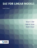
Notice that the models for one-way analysis of variance assume that the observations within each classification level are normally distributed and that the variances among the observations for each level are equal. The latter assumption was addressed in Section 3.2.3, “Two Independent Samples.” The analysis-of-variance procedure is robust, meaning that only severe failures of these assumptions compromise the results. Nonetheless, these assumptions should be checked. You can obtain simple but useful visual tools by sorting the data by classification level and running PROC UNIVARIATE. For example, for the BULLET data, use the following SAS statements:
proc sort; by powder;
proc univariate normal plot; by powder;
var velocity;
run;
Output 3.7 shows results selected for relevance.
1. Normal Probability Plots
Output 3.7 PROC UNIVARIATE Output for BULLET Data to Check ANOVA Assumptions
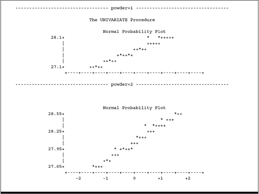
2. Side-by-Side Box-and-Whisker Plots
These plots allow you to look for strong visual evidence of failure of assumptions. You can check for non-normality using the normal probability plots. Some departure from normality is common and has no meaningful effect on ANOVA results. In fact, many statisticians argue that true normal distributions are rare in nature, if they exist at all. Highly skewed distributions, however, can seriously affect ANOVA results; strongly asymmetric box-and-whisker plots give you a useful visual cue to detect such situations. The side-by-side box-and-whisker plot also allows you to detect heterogeneous variances. Note that neither plot suggests failure of assumptions. The box-and-whisker plot does suggest that the typical response to POWDER 1 is less than the response to POWDER 2.
The UNIVARIATE output contains many other statistics, such as the variance, skewness, and kurtosis by treatment and formal tests of normality. These can be useful, for example, for testing equal variance. It is beyond the scope of this text to discuss model diagnostics in great detail. You can find such discussions in most introductory statistical methods texts. The MEANS statement of PROC GLM has an option, HOVTEST, that computes statistics to test homogeneity of variance. The GLM procedure and the MEANS statement are discussed in more detail in the remaining sections of this chapter. An example of the HOVTEST output appears in Output 3.9. In any event, you should be aware that many statisticians consider formal tests of assumptions to be of limited usefulness because the number of observations per treatment is often quite small. In most cases, strong visual evidence is the best indicator of trouble.
When analysis-of-variance assumptions fail, a common strategy involves transforming the data and computing the analysis of variance on the transformed data. Section 4.2, “Nested Classifications,” contains an example using this approach. Often, assumptions fail because the distribution of the data is known to be something other than normal. Generalized linear models are essentially regression and ANOVA models for data whose distribution is known but not necessarily normal. In such cases, you can use methods illustrated in Chapter 10, “Generalized Linear Models.”
Section 3.4.1 presents an example of analysis of variance for a one-way classification.
3.4.1 Computing the ANOVA Table
Four specimens of each of five brands (BRAND) of a synthetic wood veneer material are subjected to a friction test. A measure of wear is determined for each specimen. All tests are made on the same machine in completely random order. Data are stored in a SAS data set named VENEER.
data veneer;
input brand $ wear;
cards;
ACME 2.3
ACME 2.1
ACME 2.4
ACME 2.5
CHAMP 2.2
CHAMP 2.3
CHAMP 2.4
CHAMP 2.6
AJAX 2.2
AJAX 2.0
AJAX 1.9
AJAX 2.1
TUFFY 2.4
TUFFY 2.7
TUFFY 2.6
TUFFY 2.7
XTRA 2.3
XTRA 2.5
XTRA 2.3
XTRA 2.4
;
proc print data=veneer;
run;
Output 3.8 shows the data.
Output 3.8 Data for One-Way Classification
| Obs | brand | wear |
| 1 | ACME | 2.3 |
| 2 | ACME | 2.1 |
| 3 | ACME | 2.4 |
| 4 | ACME | 2.5 |
| 5 | CHAMP | 2.2 |
| 6 | CHAMP | 2.3 |
| 7 | CHAMP | 2.4 |
| 8 | CHAMP | 2.6 |
| 9 | AJAX | 2.2 |
| 10 | AJAX | 2.0 |
| 11 | AJAX | 1.9 |
| 12 | AJAX | 2.1 |
| 13 | TUFFY | 2.4 |
| 14 | TUFFY | 2.7 |
| 15 | TUFFY | 2.6 |
| 16 | TUFFY | 2.7 |
| 17 | XTRA | 2.3 |
| 18 | XTRA | 2.5 |
| 19 | XTRA | 2.3 |
| 20 | XTRA | 2.4 |
An appropriate analysis of variance has the basic form:
| Source of Variation | DF | |
|---|---|---|
| BRAND | 4 |
|
| Error | 15 |
|
| Total | 19 |
The following SAS statements produce the analysis of variance:
proc glm data=veneer;
class brand;
model wear=brand;
means brand/hovtest;
run;
Since the data are classified only according to the values of BRAND, this is the only variable in the CLASS statement. The variable WEAR is the response variable to be analyzed, so WEAR appears on the left side of the equal sign in the MODEL statement. The only source of variation (effect in the ANOVA table) other than ERROR (residual) and TOTAL is variation due to brands; therefore, BRAND appears on the right side of the equal sign in the MODEL statement. The MEANS statement causes the treatment means to be computed. The HOVTEST option computes statistics to test the homogeneity of variance assumption. The treatment means are not shown here; they are considered in more detail later. Output from the MODEL and HOVTEST statements appear in Output 3.9.
Output 3.9 Analysis of Variance for One-Way Classification with a Homogeneity-of-Variance Test
| The GLM Procedure | |||||
| Dependent Variable: wear | |||||
| Sum of | |||||
| Source |
DF | Squares | Mean Square | F Value | Pr > F |
| Model |
4 | 0.61700000 | 0.15425000 | 7.40 | 0.0017 |
| Error |
15 | 0.31250000 | 0.02083333 | ||
| Corrected Total |
19 | 0.92950000 | |||
| R-Square | Coeff Var | Root MSE | wear Mean |
| 0.663798 | 6.155120 | 0.144338 | 2.345000 |
| Source | DF | Type I SS | Mean Square | F Value | Pr > F |
| brand | 4 | 0.61700000 | 0.15425000 | 7.40 | 0.0017 |
| Source | DF | Type III SS | Mean Square | F Value | Pr > F |
| brand | 4 | 0.61700000 | 0.15425000 | 7.40 | 0.0017 |
| Levene's Test for Homogeneity of wear Variance ANOVA of Squared Deviations from Group Means | |||||
| Sum of | Mean | ||||
| Source | DF | Squares | Square | F Value | Pr > F |
| brand | 4 | 0.000659 | 0.000165 | 0.53 | 0.7149 |
| Error | 15 | 0.00466 | 0.000310 | ||
The results in Output 3.9 are summarized in the following ANOVA table:
| Source | DF | SS | MS | F | P |
|---|---|---|---|---|---|
| BRAND | 4 | 0.6170 | 0.1542 | 7.40 | 0.0017 |
| ERROR | 15 | 0.3125 | 0.0208 | ||
| TOTAL | 19 | 0.9295 |
Notice that you get the same computations from PROC GLM as from PROC ANOVA for the analysis of variance, although they are labeled somewhat differently. For one thing, in addition to the MODEL sum of squares, PROC GLM computes two sets of sums of squares for BRAND—Type I and Type III sums of squares—rather than the single sum of squares computed by the ANOVA procedure. For the one-way classification, as well as for balanced multiway classifications, the GLM-Type I, GLM-Type III, and PROC ANOVA sums of squares are identical. For unbalanced multiway data and for multiple regression models, the Type I and Type III SS are different. Chapter 5 discusses these differences. For the rest of this chapter, only the Type III SS will be shown in example GLM output.
The HOVTEST output appears as “Levene’s Test for Homogeneity of WEAR Variance.” The F-value, 0.53, tests the null hypothesis that the variances among observations within each treatment are equal. There is clearly no evidence to suggest failure of this assumption for these data.
3.4.2 Computing Means, Multiple Comparisons of Means, and Confidence Intervals
You can easily obtain means and multiple comparisons of means by using a MEANS statement after the MODEL statement. For the VENEER data, you get BRAND means and LSD comparisons of the BRAND means with the statement
means brand/lsd;
Results appear in Output 3.10.
Output 3.10 Least Significant Difference Comparisons of BRAND Means
| t Tests (LSD) for wear | ||
| NOTE: This test controls the Type I comparisonwise error rate, not the experimentwise error rate. | ||
| Alpha | .05 |
| Error Degrees of Freedom | 15 |
| Error Mean Square | .020833 |
| Critical Value of t | .13145 |
| Least Significant Difference | .2175 |
| Means with the same letter are not significantly different. | ||
| t Grouping | Mean | N | brand |
| A | 2.6000 | 4 | TUFFY |
| B | 2.3750 | 4 | XTRA |
| B | |||
| B | 2.3750 | 4 | CHAMP |
| B | |||
| B | 2.3250 | 4 | ACME |
| C | 2.0500 | 4 | AJAX |
Means and the number of observations (N) are produced for each BRAND. Because LSD is specified as an option, the means appear in descending order of magnitude. Under the heading “T Grouping” are sequences of A’s, B’s, and C’s. Means are joined by the same letter if they are not significantly different, according to the t-test or equivalently if their difference is less than LSD. The BRAND means for XTRA, CHAMP, and ACME are not significantly different and are joined by a sequence of B’s. The means for AJAX and TUFFY are found to be significantly different from all other means so they are labeled with a single C and A, respectively, and no other means are labeled with A’s or C’s.
You can obtain confidence intervals about means instead of comparisons of the means if you specify the CLM option:
means brand/lsd clm;
Results in Output 3.11 are self-explanatory.
Output 3.11 Confidence Intervals for BRAND Means
| t Confidence Intervals for wear | ||
| Alpha | .05 |
| Error Degrees of Freedom | 15 |
| Error Mean Square | 0.020833 |
| Critical Value of t | 2.13145 |
| Half Width of Confidence Interval | 0.153824 |
| brand | N | Mean | 95% Confidence Limits | |
| TUFFY | 4 | 2.60000 | 2.44618 | 2.75382 |
| XTRA | 4 | 2.37500 | 2.22118 | 2.52882 |
| CHAMP | 4 | 2.37500 | 2.22118 | 2.52882 |
| ACME | 4 | 2.32500 | 2.17118 | 2.47882 |
| AJAX | 4 | 2.05000 | 1.89618 | 2.20382 |
You can also obtain confidence limits for differences between means, as discussed in Section 3.5.2., “Additional Multiple Comparison Methods.”
3.4.3 Planned Comparisons for One-Way Classification: The CONTRAST Statement
Multiple comparison procedures, as demonstrated in the previous section, are useful when there are no particular comparisons of special interest and you want to make all comparisons among the means. But in most situations there is something about the classification criterion that suggests specific comparisons. For example, suppose you know something about the companies that manufacture the five brands of synthetic wood veneer material. You know that ACME and AJAX are produced by a U.S. company named A-Line, that CHAMP is produced by a U.S. company named C-Line, and that TUFFY and XTRA are produced by a non-U.S. companies.
Then you would probably be interested in comparing certain groups of means with other groups of means. For example, you would want to compare the means for the U.S. companies with the means for the non-U.S. companies; you would want to compare the means for the two U.S. companies with each other; you would want to compare the two A-Line means; and you would want to compare the means for the two non-U.S. brands. These would be called planned comparisons, because they are suggested by the structure of the classification criterion (BRAND) rather than the data. You know what comparisons you want to make before you look at the data. When this is the case, you ordinarily obtain a more relevant analysis of the data by making the planned comparisons rather than using a multiple comparison technique, because the planned comparisons are focused on the objectives of the study.
You use contrasts to make planned comparisons. In SAS, PROC ANOVA does not have a CONTRAST statement, but the GLM procedure does, so you must use PROC GLM to compute contrasts. You use CONTRAST as an optional statement the same way you use a MEANS statement.
To define contrasts and get them into a form you can use in the GLM procedure, you should first express the comparisons as null hypotheses concerning linear combinations of means to be tested. For the comparisons indicated above, you would have the following null hypotheses:
❏ U.S. versus non-U.S.
H0: 1/3(μACME + μAJAX + μCHAMP) = 1/2(μTUFFY + μXTRA)
❏ A-Line versus C-Line
H0: 1/2(μACME + μAJAX) = μCHAMP
❏ ACME versus AJAX
H0: μACME = μAJAX
❏ TUFFY versus XTRA
H0: μTUFFY = μXTRA
The basic form of the CONTRAST statement is
CONTRAST ‘label’ effect-name effect-coefficients;
where label is a character string used for labeling output, effect-name is a term on the right-hand side of the MODEL statement, and effect-coefficients is a list of numbers that specifies the linear combination of parameters in the null hypothesis. The ordering of the numbers follows the alphameric ordering (numbers first, in ascending order, then alphabetical order) of the levels of the classification variable, unless specified otherwise with an ORDER= option in the PROC GLM statement.
Starting with one of the simpler comparisons, ACME versus AJAX, you want to test H0:μACME=μAJAX. This hypothesis must be expressed as a linear combination of the means equal to 0, that is, H0: μACME – μAJAX=0. In terms of all the means, the null hypothesis is
H0: 1 * μACME – 1 * μAJAX + 0 * μCHAMP + 0 * μTUFFY + 0 * μXTRA= 0 .
Notice that the BRAND means are listed in alphabetical order. All you have to do is insert the coefficients on the BRAND means in the list of effect coefficients in the CONTRAST statement. The coefficients for the levels of BRAND follow the alphabetical ordering.
proc glm; class brand;
model wear = brand;
contrast 'ACME vs AJAX' brand 1 -1 0 0 0;
Results appear in Output 3.12.
Output 3.12 Analysis of Variance and Contrast with PROC GLM
| Contrast | DF | Contrast SS | Mean Square | F Value | Pr > F |
| ACME vs AJAX | 1 | 0.15125000 | 0.15125000 | 7.26 | 0.0166 |
Output from the CONTRAST statement, labeled ACME vs AJAX, shows a sum of squares for the contrast, and an F-value for testing H0: μACME=μAJAX. The p-value tells you the means are significantly different at the 0.0166 level.
Actually, you don’t have to include the trailing zeros in the CONTRAST statement. You can simply use
contrast 'ACME vs AJAX' brand 1 -1;
By default, if you omit the trailing coefficients they are assumed to be zeros.
Following the same procedure, to test H0: μTUFFY=μXTRA, use the statement
contrast 'TUFFY vs XTRA' brand 0 0 0 1 -1;
The contrast U.S. versus non-U.S. is a little more complicated because it involves fractions. You can use the statement
contrast 'US vs NON-U.S.' brand .33333 .33333 .33333 -.5 -.5;
Although the continued fraction for 1/3 is easily written, it is tedious. Other fractions, such as 1/7, are even more difficult to write in decimal form. It is usually easier to multiply all coefficients by the least common denominator to get rid of the fractions. This is legitimate because the hypothesis you are testing with a CONTRAST statement is that a linear combination is equal to 0, and multiplication by a constant does not change whether the hypothesis is true or false. (Something is equal to 0 if and only if a constant times the something is equal to 0.) In the case of U.S. versus non-U.S., the assertion is that
H0: 1/3(μACME + μAJAX + μCHAMP) = 1/2(μTUFFY + μXTRA)
is equivalent to
H0: 2(μACME + μAJAX + μCHAMP) – 3(μTUFFY + μXTRA) = 0
This tells you the appropriate CONTRAST statement is
contrast 'US vs NON-U.S.' brand 2 2 2 -3 -3;
The GLM procedure enables you to run as many CONTRAST statements as you want, but good statistical practice ordinarily indicates that this number should not exceed the number of degrees of freedom for the effect (in this case 4). Moreover, you should be aware of the inflation of the overall (experimentwise) Type I error rate when you run several CONTRAST statements.
To see how CONTRAST statements for all four comparisons are used, run the following program:
proc glm; class brand;
model wear = brand;
contrast 'US vs NON-U.S.' brand 2 2 2 -3 -3;
contrast 'A-L vs C-L' brand 1 1 -2 0 0;
contrast 'ACME vs AJAX' brand 1 -1 0 0 0;
contrast 'TUFFY vs XTRA' brand 0 0 0 1 -1;
run;
Output 3.13 Contrasts among BRAND Means
| Contrast | DF | Contrast SS | Mean Square | F Value | Pr > F |
| US vs NON-U.S. | 1 | 0.27075000 | 0.27075000 | 13.00 | 0.0026 |
| A-L vs C-L | 1 | 0.09375000 | 0.09375000 | 4.50 | 0.0510 |
| ACME vs AJAX | 1 | 0.15125000 | 0.15125000 | 7.26 | 0.0166 |
| TUFFY vs XTRA | 1 | 0.10125000 | 0.10125000 | 4.86 | 0.0435 |
Results in Output 3.13 indicate statistical significance for each of the contrasts. Notice that the p-value for ACME vs AJAX is the same in the presence of other CONTRAST statements as it was when run as a single contrast in Output 3.12. Computations for one CONTRAST statement are unaffected by the presence of other CONTRAST statements. The contrasts in Output 3.13 have a special property called orthogonality, which is discussed in Section 3.4.6, “Orthogonal Contrasts.”
3.4.4 Linear Combinations of Model Parameters
Thus far, the coefficients in a CONTRAST statement have been discussed as coefficients in a linear combination of means. In fact, these are coefficients on the effect parameters in the MODEL statement. It is easier to think in terms of means, but PROC GLM works in terms of model parameters. Therefore, you must be able to translate between the two sets of parameters.
Models are discussed in more depth in Chapter 4. For now, all you need to understand is the relationship between coefficients on a linear combination of means and the corresponding coefficients on linear combinations of model effect parameters. For the linear combinations representing comparisons of means (that is, with coefficients summing to 0), this relationship is very simple for the one-way classification. The coefficient of an effect parameter in a linear combination of effect parameters is equal to the coefficient on the corresponding mean in the linear combination of means. This is because of the fundamental relationship between means and effect parameters, that is, μi = μ + τi. For example, take the contrast A-Line versus C-Line. The linear combination in terms of means is
2μCHAMP – μACME– μAJAX
= 2(μ + τCHAMP) – (μ + τACME) – (μ + τAJAX)
= 2τCHAMP – τACME– τAJAX
You see that the coefficient on τCHAMP is the same as the coefficient on μCHAMP; the coefficient on τACME is equal to the coefficient on μACME, and so on. Moreover, the parameter disappears when you convert from means to effect parameters, because the coefficients on the means sum to 0.
It follows that, for comparisons in the one-way classification, you may derive coefficients in terms of means and simply insert them as coefficients on model effect parameters in a CONTRAST statement. For more complicated applications, such as two-way classifications, the task is not so straightforward. You’ll see this in Section 3.7, “A Two-Way Factorial Experiment,” and subsequent sections in this chapter.
3.4.5 Testing Several Contrasts Simultaneously
Sometimes you need to test several contrasts simultaneously. For example, you might want to test for differences among the three means for U.S. BRANDs. The null hypothesis is
H0: μACME = μAJAX = μCHAMP
This hypothesis equation actually embodies two equations that can be expressed in several ways. One way to express the hypothesis in terms of two equations is
H0: μACME = μAJAX and H0: μACME = μCHAMP
Why are the two hypotheses equivalent? Because the three means are all equal if and only if the first is equal to the second and the first is equal to the third.
You can test this hypothesis by writing a CONTRAST statement that expresses sets of coefficients for the two equations, separated by a comma. An appropriate CONTRAST statement is
contrast 'US BRANDS' brand 1 -1 0 0 0, brand 1 0 -1 0 0;
Results appear in Output 3.14.
Output 3.14 Simultaneous Contrasts among U.S. BRAND Means
| Contrast | DF | Contrast SS | Mean Square | F Value | Pr > F |
| US BRANDS | 2 | 0.24500000 | 0.12250000 | 5.88 | 0.0130 |
Notice that the sum of squares for the contrast has 2 degrees of freedom. This is because you are testing two equations simultaneously. The F-statistic of 5.88 and associated p-value tell you the means are different at the 0.0130 level of significance.
Another way to express the hypothesis in terms of two equations is
H0: μACME = μAJAX and H0: 2 μCHAMP = μACME + μAJAX
A contrast for this version of the hypothesis is
contrast 'US BRANDS' brand 1 -1 0 0 0,
brand 1 1 -2 0 0;
Results from this CONTRAST statement, not included here, are identical to Output 3.10.
3.4.6 Orthogonal Contrasts
Notice that the sum of squares, 0.245, in Output 3.14 is equal to the sum of the sums of squares for the two contrasts ACME vs AJAX (0.15125) and A-L vs C-L (0.09375) in Output 3.13. That occurs because the two sets of coefficients in this CONTRAST statement are orthogonal. Arithmetically, this means the sum of products of coefficients for the respective means is 0—that is, (1×1) + [1×(–1)] + (0×2) = 0. Moreover, all four of the contrasts in Output 3.13 form an orthogonal set. You can verify this by multiplying pairs of coefficients and adding the products. Therefore, the sum of the four contrast sums of squares in Output 3.9 is equal to the overall BRAND SS (0.617) in Output 3.9.
Statistically, orthogonal means that the sums of squares for the two contrasts are independent. The outcome of one of them in no way influences the outcome of any other. Sets of orthogonal comparisons are commonly considered desirable, because the result of any one of them tells you (essentially) nothing about what to expect from any other comparison. However, desirable as it is to have independent tests, it is more important to construct sets of contrasts to address the objectives of the investigation. Practically meaningful contrasts are more desirable than simply orthogonal ones.
3.4.7 Estimating Linear Combinations of Parameters: The ESTIMATE Statement
The CONTRAST statement is used to construct an F-test for a hypothesis that a linear combination of parameters is equal to 0. In many applications, you want to obtain an estimate of the linear combination of parameters, along with the standard error of the estimate. You can do this with an ESTIMATE statement. The ESTIMATE statement is used in much the same way as a CONTRAST statement. You could estimate the difference μACME – μAJAX with the following statement:
estimate 'ACME vs AJAX' brand 1 -1 0 0 0;
This statement is exactly like the CONTRAST statement for ACME vs AJAX, with the keyword CONTRAST replaced by the keyword ESTIMATE.
Output 3.15 Estimating the Difference between BRAND Means
| Standard | ||||
| Parameter | Estimate | Error | t Value | Pr > |t| |
| ACME vs AJAX | 0.27500000 | 0.10206207 | 2.69 | 0.0166 |
Results shown in Output 3.15 include the value of the estimate, a standard error, a t-statistic for testing whether the difference is significantly different from 0, and a p-value for the t-statistic. Note the p-value (0.0166) for the t-test is the same as for the F-test for the contrast in Output 3.12. This is because the two tests are equivalent; the F is equal to the square of the t.
For the present application, the estimate of μACME – μAJAX can be computed as
The standard error is
In more complicated examples, such as two-way classification with unbalanced data, more complicated computations for means are required.
Suppose you want to estimate μCHAMP –1/2(μACME+ μAJAX). You can use the following statement:
estimate 'AL vs CL' brand -.5 -.5 1 0 0;
The coefficients in the above ESTIMATE statement are not equivalent to the coefficients (–1 –1 2 0 0) as they would be in a CONTRAST statement. The latter set of coefficients would actually estimate twice the mean difference of interest. You can avoid the fractions by using the DIVISOR option:
estimate 'AL vs CL' brand -1 -1 2 0 0 / divisor=2;
Now suppose you want to estimate a linear combination of means that does not represent a comparison of two groups of means. For example, maybe you want to estimate the average of the three U.S. means, 1/3(μACME + μAJAX + μCHAMP). The coefficients do not sum to 0, so you can’t simply take coefficients of the means and use them in the ESTIMATE statement as coefficients on model effect parameters. The μ parameter does not disappear when you convert from means to effect parameters:
1/3(μACME + μAJAX + μCHAMP)
=1/3(μ + τACME + μ + τAJAX + μ + τCHAMP
= μ + 1/3(τACME + τAJAX + τCHAMP)
You see that the parameter ? remains in the linear combination of model effect parameters. This parameter is called INTERCEPT in CONTRAST and ESTIMATE statements. This is because ? shows up as the intercept in a regression model, as discussed in Chapter 4 where the connection between analysis-of-variance models and regression models is explained. An appropriate ESTIMATE statement is
estimate 'US MEAN' intercept 1 brand .33333 .33333 .33333 0 0;
or equivalently
estimate 'US MEAN' intercept 3 brand 1 1 1 0 0 / divisor=3;
Results from this ESTIMATE statement appear in Output 3.16.
Output 3.16 Estimating the Mean of U.S. BRANDS
| Standard | ||||
| Parameter | Estimate | Error | t Value | Pr > |t| |
| US MEAN | 2.25000000 | 0.04166667 | 54.00 | <.0001 |
In this application the estimate and its standard error are useful. For example, you can construct a 95% confidence interval:
2.25 ± 2.13(0.0417)
Again, the estimate is 2.25 = 1/3(2.325 + 2.050 + 3.375), and the standard error is [(1/4 + 1/4 + 1/4) MS(ERROR)]1/2. Since MS(ERROR) is the basic variance estimate in this formula, the degrees of freedom for the t-statistic are there for MS(ERROR). The t-statistic is computed to test the null hypothesis
H0: μACME + μAJAX + μCHAMP = 0
Of course, this hypothesis is not of practical interest.
3.5 Randomized-Blocks Designs
The randomized-blocks design assumes that a population of experimental units can be divided into a relatively homogeneous subpopulations that are called blocks. The treatments are then randomly assigned to experimental units within the blocks. If all treatments are assigned in each block, the design is called a randomized-complete-blocks design. Blocks usually represent naturally occurring differences not related to the treatments. In analysis of variance, the extraneous variation among blocks can be partitioned out, usually reducing the error mean square. Also, differences between treatment means do not contain block variation. In this sense, the randomized-blocks design controls block variation.
A classic example of blocks is an agricultural field that is divided into smaller, more homogeneous subfields. Other examples of blocks include days of the week, measuring or recording devices, and operators of a machine. The paired two-sample design, such as the PULSE data in Section 3.2.2, “Two Related Samples,” is a special case of the randomized-complete-blocks design with the two samples as treatments and pairs as the blocks.
In the following example, five methods of applying irrigation (IRRIG) are applied to a Valencia orange tree grove. The trees in the grove are arranged in eight blocks (BLOC) to account for local variation. That is, variation among trees within a block is minimized. Assignment of the irrigation method to trees within each block is random, giving a randomized-blocks design. Each of the five irrigation methods appears in all eight blocks and there are no missing data, making this a randomized-complete-blocks design. At harvest, for each plot the fruit is weighed in pounds. The objective is to determine if method of irrigation affects fruit weight (FRUITWT) and to rank the irrigation treatments accordingly.
The data appear in Output 3.17. The following SAS DATA step often provides a convenient shortcut for data entry, because it allows you to put the data for all eight blocks on a single line for each treatment. You can modify these statements to put the data for all treatments on a single line for each block.
data methods;
input irrig $ @@;
do bloc=1 to 8;
input fruitwt @@;
output;
end;
datalines;
trickle 450 469 249 125 280 352 221 251
basin 358 512 281 58 352 293 283 186
spray 331 402 183 70 258 281 219 46
sprnkler 317 423 379 63 289 239 269 357
flood 245 380 263 62 336 282 171 98
;
proc sort;
by bloc irrig;
proc print;
var bloc irrig fruitwt;
run;
Output 3.17 Data for the Randomized-Complete-Blocks Design
| Obs | bloc | irrig | fruitwt |
| 1 | 1 | basin | 358 |
| 2 | 1 | flood | 245 |
| 3 | 1 | spray | 331 |
| 4 | 1 | sprnkler | 317 |
| 5 | 1 | trickle | 450 |
| 6 | 2 | basin | 512 |
| 7 | 2 | flood | 380 |
| 8 | 2 | spray | 402 |
| 9 | 2 | sprnkler | 423 |
| 10 | 2 | trickle | 469 |
| 11 | 3 | basin | 281 |
| 12 | 3 | flood | 263 |
| 13 | 3 | spray | 183 |
| 14 | 3 | sprnkler | 379 |
| 15 | 3 | trickle | 249 |
| 16 | 4 | basin | 58 |
| 17 | 4 | flood | 62 |
| 18 | 4 | spray | 70 |
| 19 | 4 | sprnkler | 63 |
| 20 | 4 | trickle | 125 |
| 21 | 5 | basin | 352 |
| 22 | 5 | flood | 336 |
| 23 | 5 | spray | 258 |
| 24 | 5 | sprnkler | 289 |
| 25 | 5 | trickle | 280 |
| 26 | 6 | basin | 293 |
| 27 | 6 | flood | 282 |
| 28 | 6 | spray | 281 |
| 29 | 6 | sprnkler | 239 |
| 30 | 6 | trickle | 352 |
| 31 | 7 | basin | 283 |
| 32 | 7 | flood | 171 |
| 33 | 7 | spray | 219 |
| 34 | 7 | sprnkler | 269 |
| 35 | 7 | trickle | 221 |
| 36 | 8 | basin | 186 |
| 37 | 8 | flood | 98 |
| 38 | 8 | spray | 46 |
| 39 | 8 | sprnkler | 357 |
| 40 | 8 | trickle | 251 |
3.5.1 Analysis of Variance for Randomized-Blocks Design
The following analysis of variance for the randomized-complete-blocks design provides a test for the differences among irrigation methods:
| Source | DF |
|---|---|
| BLOC | 7 |
| IRRIG | 4 |
| ERROR | 28 |
| TOTAL | 39 |
Use the following SAS statements to compute the basic analysis of variance:
proc glm;
class bloc irrig;
model fruitwt=bloc irrig;
BLOC and IRRIG appear in the CLASS statement because the data are classified according to these variables. The MODEL statement specifies that the response variable to be analyzed is FRUITWT. The two sources of variation in the analysis-of-variance table (other than ERROR and TOTAL) are BLOC and IRRIG, so these variables appear on the right side of the MODEL statement. The analysis appears in Output 3.18.
Output 3.18 Analysis of Variance for the Randomized-Complete-Blocks Design
| Dependent Variable: wear | |||||
| Sum of | |||||
| Source | DF | Squares | Mean Square | F Value | Pr > F |
| Model | 11 | 445334.0250 | 40484.9114 | 12.04 | <.0001 |
| Error | 28 | 94146.7500 | 3362.3839 | ||
| Corrected Total | 39 | 539480.7750 | |||
| R-Square | Coeff Var | Root MSE | wear Mean |
| 0.825486 | 21.71153 | 57.98607 | 267.0750 |
| Source | DF | Type I SS | Mean Square | F Value | Pr > F |
| bloc | 7 | 401308.3750 | 57329.7679 | 17.05 | <.0001 |
| irrig | 4 | 44025.6500 | 11006.4125 | 3.27 | 0.0254 |
| Source | DF | Type III SS | Mean Square | F Value | Pr > F |
| bloc | 7 | 401308.3750 | 57329.7679 | 17.05 | <.0001 |
| irrig | 4 | 44025.6500 | 11006.4125 | 3.27 | 0.0254 |
The top section contains lines labeled MODEL, ERROR, and CORRECTED TOTAL. The total variation, as measured by the total sum of squares, is partitioned into two components: variation due to the effects in the model (MODEL) and variation not due to effects in the model (ERROR). The bottom section of the output contains lines labeled BLOC and IRRIG. These partition the MODEL sum of squares into two components: sum of squares due to the effects of blocks (BLOC) and sum of squares due to the effects of treatment (IRRIG). In most cases when MODEL is partitioned into two or more sources of variation, the F-test for MODEL has no useful interpretation; you want to interpret the BLOC and IRRIG sources of variation separately.
In the GLM output, there are two sets of sums of squares, TYPE I and TYPE III. For balanced data such as the randomized-complete-blocks design with no missing data, these sums of square types are identical. In analysis of variance, the types of sum of squares matter when the data are unbalanced. An example is when you have missing data or incomplete-blocks designs. Chapter 5 discusses the different types of sums of squares.
You can summarize the key features of Output 3.18 in the following ANOVA table:
| Source | DF | SS | MS | F | p-value |
|---|---|---|---|---|---|
| BLOC | 7 | 401308.375 | |||
| IRRIG | 4 | 44025.650 | 11006.4125 | 3.27 | 0.0254 |
| ERROR | 28 | 94146.750 | 3362.3839 | ||
| TOTAL | 39 | 539480.775 |
3.5.2 Additional Multiple Comparison Methods
In Section 3.4, “The Analysis of One-Way Classification of Data,” you saw how to compare treatment means using least significant difference tests, basically two-sample t-tests in the context of analysis of variance, and contrasts. In addition, there are many multiple comparison tests available in PROC ANOVA and PROC GLM. It bears repeating that you should use contrasts whenever the structure of the treatment design permits, and it is usually advisable to structure the treatment design to facilitate using contrasts tailored to the specific objectives of the study. However, there are many situations where no obvious structure exists, and imposing structure would be artificial and inappropriate. These are the cases for which you should use multiple comparison tests.
In this section the randomized-blocks example shown above is used to illustrate some of these tests. The tests illustrated in this example are summarized below, including information pertaining to their error rates and option keywords.
❏ Least Significant Difference (LSD)
comparisonwise error rate (ALPHA=probability of Type I error for any one particular comparison)
❏ Duncan’s New Multiple Range (DUNCAN)
error rate comparable to k–1 orthogonal comparisons tested simultaneously
❏ Waller-Duncan (WALLER)
error rate dependent on value of analysis-of-variance F-test
❏ Tukey’s Honest Significant Difference (TUKEY)
experimentwise error rate (ALPHA=probability of one or more Type I errors altogether).
You may wonder why there are so many different tests. In mean comparisons, two types of error are possible. The test may incorrectly declare treatment means that are actually equal to be different; this is called a Type I error. Or the test may fail to declare a difference between treatment means that are not equal; this is called a Type II error. Multiple comparison tests differ in their Type I error rate, that is, the probability of incorrectly declaring treatment means to be different. The LSD test has the highest Type I error rate and Tukey’s the lowest, with Duncan and Waller-Duncan in the middle. When Type I error rate is reduced, all other things being equal, Type II error rate increases. The reason for so many tests is that different situations call for different priorities. For example, in the early stages of research, when you may be trying to identify new treatments that show any evidence of promise, Type I error may not be serious because follow-up research will reveal spurious differences. However, Type II error is serious because a potentially valuable treatment will go unnoticed. On the other hand, in later stages of research, Type I error may be much more serious, because it may mean allowing an ineffective product to be recommended as if it were effective, possibly with tragic consequences. As you can imagine, there is no one “correct” test for all situations—you must evaluate each case based on the relative consequences of Type I and Type II error.
For the LSD, DUNCAN, and TUKEY options, ALPHA=.05 unless the ALPHA= option is specified. Only ALPHA= values of .01, .05, or .1 are allowed with the Duncan’s test. The Waller test is based on Bayesian principles and utilizes the Type I/Type II error seriousness ratio, called the k-ratio, instead of an ALPHA=value. In practice, ALPHA=.05 for the DUNCAN option and KRATIO=100 for the WALLER option produce similar results.
The following SAS statements illustrate the options:
proc glm;
class bloc irrig;
model fruitwt=bloc irrig;
means irrig/duncan lsd tukey waller;
means irrig/duncan tukey alpha=0.1;
Note that you can ask for more than one multiple comparison option for a given ALPHA level in the same MEANS statement. The results in Output 3.19 reveal that, among the methods illustrated, the LSD option tends to produce the most significant differences, the TUKEY option tends to produce the least, and the DUNCAN tends to be somewhere in between.
1. LSD
Output 3.19 Several Types of Multiple Comparison Procedures
| t Tests (LSD) for fruitwt | ||
| NOTE: This test controls the Type I comparisonwise error rate, not the experimentwise error rate. | ||
| Alpha | 0.05 |
| Error Degrees of Freedom | 28 |
| Error Mean Square | 3362.384 |
| Critical Value of t | 2.04841 |
| Least Significant Difference | 59.39 |
| Means with the same letter are not significantly different. |
| t Grouping | Mean | N | irrig |
| A | 299.63 | 8 | trickle |
| A | |||
| A | 292.00 | 8 | sprnkler |
| A | |||
| A | 290.38 | 8 | basin |
| B | 229.63 | 8 | flood |
| B | |||
| B | 223.75 | 8 | spray |
2. DUNCAN
| Duncan's Multiple Range Test for fruitwt | ||
| NOTE: This test controls the Type I comparisonwise error rate, not the experimentwise error rate. | ||
| Alpha | 0.05 |
| Error Degrees of Freedom | 28 |
| Error Mean Square | 3362.384 |
| Number of Means | 2 | 3 | 4 | 5 |
| Critical Range | 59.39 | 62.40 | 64.35 | 65.74 |
| Means with the same letter are not significantly different. | ||
| Duncan Grouping | Mean | N | irrig | |
| A | 299.63 | 8 | trickle | |
| A | ||||
| B | A | 292.00 | 8 | sprnkler |
| B | A | |||
| B | A | 290.38 | 8 | basin |
| B | ||||
| B | C | 229.63 | 8 | flood |
| C | ||||
| C | 223.75 | 8 | spray | |
3. WALLER
| Waller-Duncan K-ratio t Test for fruitwt | ||
| NOTE: This test minimizes the Bayes risk under additive loss and certain other assumptions. | ||
| Kratio | 100 |
| Error Degrees of Freedom | 28 |
| Error Mean Square | 3362.384 |
| F Value | 3.27 |
| Critical Value of t | 2.23982 |
| Minimum Significant Difference | 64.939 |
| Means with the same letter are not significantly different. | ||
| Waller Grouping | Mean | N | irrig | |
| A | 299.63 | 8 | trickle | |
| A | ||||
| B | A | 292.00 | 8 | sprnkler |
| B | A | |||
| B | A | 290.38 | 8 | basin |
| B | ||||
| B | C | 229.63 | 8 | flood |
| C | ||||
| C | 223.75 | 8 | spray | |
4. TUKEY
| Tukey's Studentized Range (HSD) Test for fruitwt | ||
| NOTE: This test controls the Type I experimentwise error rate, but it generally has a higher Type II error rate than REGWQ. | ||
| Alpha | 0.05 |
| Error Degrees of Freedom | 28 |
| Error Mean Square | 3362.384 |
| Critical Value of Studentized Range | 4.12030 |
| Minimum Significant Difference | 84.471 |
| Means with the same letter are not significantly different. |
| Tukey Grouping | Mean | N | irrig |
| A | 299.63 | 8 | trickle |
| A | |||
| A | 292.00 | 8 | sprnkler |
| A | |||
| A | 290.38 | 8 | basin |
| A | |||
| A | 229.63 | 8 | flood |
| A | |||
| A | 223.75 | 8 | spray |
5. DUNCAN with Type I error level set to ALPHA=0.10
| Duncan's Multiple Range Test for fruitwt | ||
| NOTE: This test controls the Type I comparisonwise error rate, not the experimentwise error rate. | ||
| Alpha | 0.05 |
| Error Degrees of Freedom | 28 |
| Error Mean Square | 3362.384 |
| Number of Means | 2 | 3 | 4 | 5 |
| Critical Range | 49.32 | 52.01 | 53.71 | 54.90 |
| Means with the same letter are not significantly different. |
| Duncan Grouping | Mean | N | irrig |
| A | 299.63 | 8 | trickle |
| A | |||
| A | 292.00 | 8 | sprnkler |
| A | |||
| A | 290.38 | 8 | basin |
| B | 229.63 | 8 | flood |
| B | |||
| B | 223.75 | 8 | spray |
6. TUKEY with Type I error level set to ALPHA=0.10
| Tukey's Studentized Range (HSD) Test for fruitwt | ||
| NOTE: This test controls the Type I experimentwise error rate, but it generally has a higher Type II error rate than REGWQ. | ||
| Alpha | 0.1 |
| Error Degrees of Freedom | 28 |
| Error Mean Square | 3362.384 |
| Critical Value of Studentized Range | 3.66039 |
| Minimum Significant Difference | 75.042 |
| Means with the same letter are not significantly different. |
| Tukey Grouping | Mean | N | irrig | |
| A | 299.63 | 8 | trickle | |
| A | ||||
| B | A | 292.00 | 8 | sprnkler |
| B | A | |||
| B | A | 290.38 | 8 | basin |
| B | A | |||
| B | A | 229.63 | 8 | flood |
| B | ||||
| B | 223.75 | 8 | spray | |
Some multiple comparison results can be expressed as confidence intervals for differences between pairs of means. This provides more information regarding the differences than simply joining nonsignificantly different means with a common letter, but more space is required to print the results. Specifying the CLDIFF option selects the confidence interval option. For example, the following SAS statement produces Output 3.20:
means irrig/tukey alpha=0.1 cldiff;
Output 3.20 Simultaneous Confidence Intervals for Differences
| Tukey's Studentized Range (HSD) Test for fruitwt | ||
| NOTE: This test controls the Type I experimentwise error rate. | ||
| Alpha | 0.1 |
| Error Degrees of Freedom | 28 |
| Error Mean Square | 3362.384 |
| Critical Value of Studentized Range | 3.66039 |
| Minimum Significant Difference | 75.042 |
| Comparisons significant at the 0.1 level are indicated by *** | ||
| irrig Comparison |
Difference Between Means |
Simultaneous 90% Confidence Limits |
|||
| trickle | - sprnkler | 7.63 | -67.42 | 82.67 | |
| trickle | - basin | 9.25 | -65.79 | 84.29 | |
| trickle | - flood | 70.00 | -5.04 | 145.04 | |
| trickle | - spray | 75.88 | 0.83 | 150.92 | *** |
| sprnkler | - trickle | -7.63 | -82.67 | 67.42 | |
| sprnkler | - basin | 1.63 | -73.42 | 76.67 | |
| sprnkler | - flood | 62.38 | -12.67 | 137.42 | |
| sprnkler | - spray | 68.25 | -6.79 | 143.29 | |
| basin | - trickle | -9.25 | -84.29 | 65.79 | |
| basin | - sprnkler | -1.63 | -76.67 | 73.42 | |
| basin | - flood | 60.75 | -14.29 | 135.79 | |
| basin | - spray | 66.63 | -8.42 | 141.67 | |
| flood | - trickle | -70.00 | -145.04 | 5.04 | |
| flood | - sprnkler | -62.38 | -137.42 | 12.67 | |
| flood | - basin | -60.75 | -135.79 | 14.29 | |
| flood | - spray | 5.88 | -69.17 | 80.92 | |
| spray | - trickle | -75.88 | -150.92 | -0.83 | *** |
| spray | - sprnkler | -68.25 | -143.29 | 6.79 | |
| spray | - basin | -66.63 | -141.67 | 8.42 | |
| spray | - flood | -5.88 | -80.92 | 69.17 | |
The three asterisks (***) appear to the right of each difference whose confidence interval does not include 0. Such confidence intervals, for instance TRICKLE-SPRAY and SPRAY-TRICKLE in Output 3.20, indicate the difference is significant at the ALPHA rate. The confidence interval method of presentation is the default for some methods when the means are based on different numbers of observations because the required difference for significance depends on the numbers of observations in the means.
3.5.3 Dunnett’s Test to Compare Each Treatment to a Control
In some experiments, the primary objective is to screen treatments by making pairwise comparisons of each treatment to a “control” or reference treatment. For example, Keuhl (2000) notes that for the Valencia orange irrigation data, FLOOD is the standard method and hence the reference treatment against which the others are to be evaluated.
Dunnett’s procedure is a specialized procedure intended to control experimentwise error rate when mean comparisons are limited to pairwise tests between the reference treatment and each other treatment. The MEANS statement provides a DUNNETT option, that is, you use the SAS statement
means irrig/dunnett alpha=0.1;
The ALPHA=0.1 is optional. If you omit it, the default α – level is 0.05. Output 3.21 shows the result.
Output 3.21 Dunnett’s Test for Differences between Reference and Other Treatments
| Dunnett's t Tests for fruitwt | ||
| NOTE: This test controls the Type I experimentwise error for comparisons of all treatments against a control. | ||
| Alpha | 0.1 |
| Error Degrees of Freedom | 28 |
| Error Mean Square | 3362.384 |
| Critical Value of Dunnett's t | 2.26128 |
| Minimum Significant Difference | 65.561 |
| Comparisons significant at the 0.1 level are indicated by ***. | ||
| irrig Comparison |
Difference Between Means |
Simultaneous 90% Confidence Limits |
|||
| trickle | - basin | 9.25 | -56.31 | 74.81 | |
| sprnkler | - basin | 1.63 | -63.94 | 67.19 | |
| flood | - basin | -60.75 | -126.31 | 4.81 | |
| spray | - basin | -66.63 | -132.19 | -1.06 | *** |
The style of Output 3.21 is similar to the confidence interval presentation for the Tukey procedure shown in Output 3.20. Three asterisks indicate significant treatment differences, or equivalently, confidence intervals that do not include 0. In this case, the SPRAY-BASIN difference is statistically significant at α = 0.10.
Note, however, that BASIN was used as the reference, not FLOOD, as required by the objectives. The default for the Dunnett procedure is to use the first treatment in alphameric order as the reference. If you want another treatment to be used as the control, you need to modify the MEANS statement by including an option that names the reference treatment:
means irrig/dunnett ('flood') alpha=0.1;
Output 3.22 shows the modified Dunnett procedure.
Output 3.22 The Dunnett Procedure with FLOOD Specified as the Control
| Dunnett's t Tests for fruitwt | ||
| NOTE: This test controls the Type I experimentwise error for comparisons of all treatments against a control. | ||
| Alpha | 0.1 |
| Error Degrees of Freedom | 28 |
| Error Mean Square | 3362.384 |
| Critical Value of Dunnett's t | 2.26128 |
| Minimum Significant Difference | 65.561 |
| Comparisons significant at the 0.1 level are indicated by ***. | ||
| irrig Comparison |
Difference Between Means |
Simultaneous 90% Confidence Limits |
|||
| trickle | - flood | 70.00 | 4.44 | 135.56 | *** |
| sprnkler | - flood | 62.38 | -3.19 | 127.94 | |
| basin | - flood | 60.75 | -4.81 | 126.31 | |
| spray | - flood | -5.88 | -71.44 | 59.69 | |
You can see from this output that only the TRICKLE treatment yields a greater mean fruit weight by a margin that is statistically significant at α =0.10.
3.6 A Latin Square Design with Two Response Variables
As described in Section 3.5, the randomized-blocks design controls one source of extraneous variation. It often happens, however, that there are two or more identifiable sources of variation. Such a situation may call for a Latin square design. The Latin square design is a special case of the more general row-column design, which controls two sources of extraneous variation, usually referred to as rows and columns. The Latin square is an orthogonal design, so that PROC ANOVA, and GLM Type I and Type III sums of square yield equivalent results. Treatments are randomly assigned to experimental units with the restriction that each treatment occurs once in each row and once in each column.
Consider the following example of a Latin square: Four materials (A, B, C, and D) used in permanent-press garments are subjected to a test for weight loss and shrinkage. The four materials (MAT) are placed in a heat chamber that has four control settings or positions (POS). The test is conducted in four runs (RUN), with each material assigned to each of the four positions in one execution of the experiment:
| Run | Position | |||
|---|---|---|---|---|
| 1 | 2 | 3 | 4 | |
| 1 | B | D | A | C |
| 2 | D | B | C | A |
| 3 | A | C | B | D |
| 4 | C | A | D | B |
The weight loss (WTLOSS) and shrinkage (SHRINK) are measured on each sample following each test. The data appear in Output 3.23.
Output 3.23 Data for the Latin Square Design
| Obs | run | pos | mat | wtloss | shrink |
| 1 | 2 | 4 | A | 251 | 50 |
| 2 | 2 | 2 | B | 241 | 48 |
| 3 | 2 | 1 | D | 227 | 45 |
| 4 | 2 | 3 | C | 229 | 45 |
| 5 | 3 | 4 | D | 234 | 46 |
| 6 | 3 | 2 | C | 273 | 54 |
| 7 | 3 | 1 | A | 274 | 55 |
| 8 | 3 | 3 | B | 226 | 43 |
| 9 | 1 | 4 | C | 235 | 45 |
| 10 | 1 | 2 | D | 236 | 46 |
| 11 | 1 | 1 | B | 218 | 43 |
| 12 | 1 | 3 | A | 268 | 51 |
| 13 | 4 | 4 | B | 195 | 39 |
| 14 | 4 | 2 | A | 270 | 52 |
| 15 | 4 | 1 | C | 230 | 48 |
| 16 | 4 | 3 | D | 225 | 44 |
The following table shows the sources of variation and degrees of freedom for an analysis of variance for the Latin square design:
| Source | DF |
|---|---|
| RUN | 3 |
| POS | 3 |
| MAT | 3 |
| ERROR | 6 |
Use the following SAS statements to obtain the analysis of variance:
proc glm data=garments;
class run pos mat;
model wtloss shrink = run pos mat;
run;
The data are classified according to RUN, POS, and MAT, so these variables appear in the CLASS statement. The response variables to be analyzed are WTLOSS and SHRINK, and the sources of variation in the ANOVA table are RUN, POS, and MAT. Note that one MODEL statement handles both response variables simultaneously. Output 3.24 shows the results.
Output 3.24 Analysis of Variance for the Latin Square Design
| Dependent Variable: wtloss | |||||
| Sum of | |||||
| Source | DF | Squares | Mean Square | F Value | Pr > F |
| Model | 9 | 7076.500000 | 786.277778 | 12.84 | 0.0028 |
| Error | 6 | 367.500000 | 61.250000 | ||
| Corrected Total | 15 | 7444.000000 | |||
| R-Square | Coeff Var | Root MSE | wtloss Mean |
| 0.950631 | 3.267740 | 7.826238 | 239.5000 |
| Source | DF | Type III SS | Mean Square | F Value | Pr > F |
| run | 3 | 986.500000 | 328.833333 | 5.37 | 0.0390 |
| pos | 3 | 1468.500000 | 489.500000 | 7.99 | 0.0162 |
| mat | 3 | 4621.500000 | 1540.500000 | 25.15 | 0.0008 |
| Dependent Variable shrink | |||||
| Sum of | |||||
| Source | DF | Squares | Mean Square | F Value | Pr > F |
| Model | 9 | 265.7500000 | 29.5277778 | 9.84 | 0.0058 |
| Error | 6 | 18.0000000 | 3.0000000 | ||
| Corrected Total | 15 | 283.7500000 | |||
| R-Square | Coeff Var | Root MSE | wtloss Mean |
| 0.936564 | 3.675439 | 1.732051 | 47.12500 |
| Source | DF | Type III SS | Mean Square | F Value | Pr > F |
| run | 3 | 33.2500000 | 11.0833333 | 3.69 | 0.0813 |
| pos | 3 | 60.2500000 | 20.0833333 | 6.69 | 0.0242 |
| mat | 3 | 172.2500000 | 57.4166667 | 19.14 | 0.0018 |
The following table is a summary of the results.
| WTLOSS Source |
DF | SS | MS | F | p |
|---|---|---|---|---|---|
| RUN | 3 | 986.5 | |||
| POS | 3 | 1468.5 | |||
| MAT | 3 | 4621.5 | 1540.5 | 25.15 | 0.0008 |
| ERROR | 6 | 367.5 | 61.25 | ||
| TOTAL | 15 | 7444.0 | |||
| SHRINK Source |
DF | SS | MS | F | p |
| RUN | 3 | 33.25 | |||
| POS | 3 | 60.25 | |||
| MAT | 3 | 172.25 | 57.42 | 19.14 | 0.0018 |
| ERROR | 6 | 18.00 | 3.00 | ||
| TOTAL | 15 | 283.75 |
The F-tests for MAT indicate differences between materials in both WTLOSS and SHRINK. For a more detailed discussion of Latin square designs, see Steel and Torrie (1980).
3.7 A Two-Way Factorial Experiment
Two of the basic aspects of the design of experiments are treatment structure and error control. Choosing between randomization schemes, such as completely randomized, randomized blocks, and so on, is part of error control. This aspect is sometimes called the experiment design. On the other hand the structure of the treatments, what factor(s) and factor levels are to be observed is called the treatment design. The factorial treatment design is one of the most important and widely used treatment structures. The factorial treatment design can be used with any randomization scheme, or experiment design. This section introduces the analysis of variance and mean comparison procedures used with factorial experiments.
A complete factorial experiment consists of all possible combinations of levels of two or more variables. Levels can refer to numeric quantities of variables, such as pounds of fertilizer ingredients or degrees of temperature, as well as qualitative categories, such as names of breeds or drugs. Variables, which are called factors, can be different fertilizer ingredients (N, P, K), operating conditions (temperature, pressure), biological factors (breeds, varieties), or any combination of these. An example of a factorial experiment is a study using nitrogen, phosphorus, and potassium, each at three levels. Such an experiment has 33= 27 treatment combinations.
Factorial experiments can be used to investigate several types of treatment effects. Following from the discussion of sums of squares and related terminology in Section 3.3.1, these are
❏ simple effects, that is, how levels of one factor affect the response variable holding the other factor constant at a given level
❏ interactions, that is, how levels of one factor affect the response variable across levels of another factor—do the simple effects remain constant (no interaction) or do they change (interaction)
❏ main effects, that is, overall differences between levels of each factor averaged over all the levels of the other factor.
For example, suppose three seed growth-promoting methods (METHOD) are applied to seed from each of five varieties (VARIETY) of turf grass. Six pots are planted with seed from each METHOD×VARIETY combination. The resulting 90 pots are randomly placed in a uniform growth chamber and the dry matter yields (YIELD) are measured after clipping at the end of four weeks. In this experiment, the concern is only about these five varieties and three growth methods. VARIETY and METHOD are regarded as fixed effects. A complete description of the experiment, for example, for a scientific article, includes the treatment design, a 3×5 factorial, and the randomization scheme, a completely randomized design. The two factors are METHOD and VARIETY.
Data are recorded in a SAS data set called GRASSES, which appears in Output 3.25. For convenience, the six replicate measurements are recorded as Y1-Y6 in the same data line.
Output 3.25 Data for the Factorial Experiment
| Obs | method | variety | y1 | y2 | y3 | y4 | y5 | y6 | trt |
| 1 | a | 1 | 22.1 | 24.1 | 19.1 | 22.1 | 25.1 | 18.1 | a1 |
| 2 | a | 2 | 27.1 | 15.1 | 20.6 | 28.6 | 15.1 | 24.6 | a2 |
| 3 | a | 3 | 22.3 | 25.8 | 22.8 | 28.3 | 21.3 | 18.3 | a3 |
| 4 | a | 4 | 19.8 | 28.3 | 26.8 | 27.3 | 26.8 | 26.8 | a4 |
| 5 | a | 5 | 20.0 | 17.0 | 24.0 | 22.5 | 28.0 | 22.5 | a5 |
| 6 | b | 1 | 13.5 | 14.5 | 11.5 | 6.0 | 27.0 | 18.0 | b1 |
| 7 | b | 2 | 16.9 | 17.4 | 10.4 | 19.4 | 11.9 | 15.4 | b2 |
| 8 | b | 3 | 15.7 | 10.2 | 16.7 | 19.7 | 18.2 | 12.2 | b3 |
| 9 | b | 4 | 15.1 | 6.5 | 17.1 | 7.6 | 13.6 | 21.1 | b4 |
| 10 | b | 5 | 21.8 | 22.8 | 18.8 | 21.3 | 16.3 | 14.3 | b5 |
| 11 | c | 1 | 19.0 | 22.0 | 20.0 | 14.5 | 19.0 | 16.0 | c1 |
| 12 | c | 2 | 20.0 | 22.0 | 25.5 | 16.5 | 18.0 | 17.5 | c2 |
| 13 | c | 3 | 16.4 | 14.4 | 21.4 | 19.9 | 10.4 | 21.4 | c3 |
| 14 | c | 4 | 24.5 | 16.0 | 11.0 | 7.5 | 14.5 | 15.5 | c4 |
| 15 | c | 5 | 11.8 | 14.3 | 21.3 | 6.3 | 7.8 | 13.8 | c5 |
3.7.1 ANOVA for a Two-Way Factorial Experiment
An analysis of variance for the experiment has the following form:
| Source | DF |
|---|---|
| METHOD | 2 |
| VARIETY | 4 |
| METHOD×VARIETY | 8 |
| ERROR | 75 |
The METHOD×VARIETY interaction is a measure of whether differences among METHOD means depend on the VARIETY being used. If the interaction is present, it may be necessary to compare METHOD means separately for each VARIETY, that is, evaluate the simple effects of METHOD|VARIETY. If the interaction is not present, a comparison of METHOD averaged over all levels of VARIETY, that is, the main effect of METHOD, is appropriate.
Because a single YIELD value is needed for each observation instead of six values, the data set GRASSES shown in Output 3.25 must be rearranged to permit analysis. This data manipulation would not be necessary if the values of YIELD had originally been recorded using one data line per replication. Use the following SAS statements to rearrange the data:
data fctorial; set grasses; drop y1-y6;
yield=y1; output;
yield=y2; output;
yield=y3; output;
yield=y4; output;
yield=y5; output;
yield=y6; output;
run;
This creates a new data set, named FCTORIAL, containing the rearranged data. The following SAS statements sort the data by METHOD and VARIETY, and then compute and plot means for visual inspection:
proc sort;
by method variety;
proc means data=fctorial noprint;
by method variety;
output out=factmean mean=yldmean;
proc print data=factmean;
run;
The PROC MEANS statement instructs SAS to compute means and standard errors of the means of each METHOD×VARIETY combination. Note that you must first use PROC SORT to sort the data in the same order as the BY statement used with PROC MEANS. The NOPRINT option suppresses PROC MEANS from printing its computations. The OUTPUT statement creates a new SAS data set named FACTMEAN. The MEAN= option creates a new variable named YLDMEAN, whose values are the means of the variable YIELD for each combination of the values of the variables METHOD and VARIETY. The data set FACTMEAN appears in Output 3.26.
Output 3.26 Cell Means for the Factorial Experiment
| Obs | method | variety | _TYPE_ | _FREQ_ | yldmean |
| 1 | a | 1 | 0 | 6 | 21.7667 |
| 2 | a | 2 | 0 | 6 | 21.8500 |
| 3 | a | 3 | 0 | 6 | 23.1333 |
| 4 | a | 4 | 0 | 6 | 25.9667 |
| 5 | a | 5 | 0 | 6 | 22.3333 |
| 6 | b | 1 | 0 | 6 | 15.0833 |
| 7 | b | 2 | 0 | 6 | 15.2333 |
| 8 | b | 3 | 0 | 6 | 15.4500 |
| 9 | b | 4 | 0 | 6 | 13.5000 |
| 10 | b | 5 | 0 | 6 | 19.2167 |
| 11 | c | 1 | 0 | 6 | 18.4167 |
| 12 | c | 2 | 0 | 6 | 19.9167 |
| 13 | c | 3 | 0 | 6 | 17.3167 |
| 14 | c | 4 | 0 | 6 | 14.8333 |
| 15 | c | 5 | 0 | 6 | 12.5500 |
You can use PROC PLOT or PROC GPLOT to plot YLDMEAN in order to visually show METHOD and VARIETY effects. The following statements cause PROC PLOT to make a low-resolution plot of the mean yields for each variety:
proc plot data=factmean;
plot yldmean*variety=method;
The PLOT statement plots the values of YLDMEAN on the vertical axis versus the VARIETY values on the horizontal axis and labels the points according to METHOD names A, B, or C. You can use PROC GPLOT to construct a higher resolution version of this interaction plot, which appears in Output 3.27. Use the statements
axis1 value=(font=swiss2 h=2) label=(f=swiss h=2 'Mean
Yield'),
axis2 value=(font=swiss h=2) label=(f=swiss h=2 'Variety'),
legend1 value=(font=swiss h=2) label=(f=swiss h=2 'Method'),
symbol1 color=black interpol =join
line=1 value='A' font=swiss;
symbol2 color=black interpol=join
line=2 value='B' font=swiss;
symbol3 color=black interpol=join
line=20 value='C' font=swiss;
proc gplot data=factmean;
plot yldmean*variety=method/caxis=black ctext=black
axis=axis1 haxis=axis2 legend=legend1;
Output 3.27 Plots of Cell Mean for the Factorial Experiment
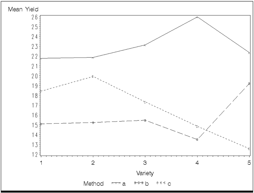
The interaction plot suggests that the magnitude of differences between METHOD means depends on which VARIETY is used. This should be formally tested, however, since the graph only shows treatment means, not their underlying variation.
Run the following SAS statements to compute the analysis:
proc glm data=fctorial;
class method variety;
model yield=method variety method*variety;
run;
Note that both treatment factors, METHOD and VARIETY, are classification variables and thus appear in the CLASS statement. The MODEL statement specifies that the analysis of YIELD contain sources of variation METHOD, VARIETY, and METHOD*VARIETY. You can see that the syntax for interaction is factor A*factor B.
Output 3.28 contains the results.
Output 3.28 Analysis of Variance for the Factorial Experiment
| Dependent Variable: yield | |||||
| Sum of | |||||
| Source | DF | Squares | Mean Square | F Value | Pr > F |
| Model | 14 | 1339.024889 | 95.644635 | 4.87 | <.0001 |
| Error | 75 | 1473.766667 | 19.650222 | ||
| Corrected Total | 89 | 2812.791556 | |||
| R-Square | Coeff Var | Root MSE | wtloss Mean |
| 0.476048 | 24.04225 | 4.432857 | 18.43778 |
| Source | DF | Type III SS | Mean Square | F Value | Pr > F |
| method | 2 | 953.1562222 | 476.5781111 | 24.25 | <.0001 |
| variety | 4 | 11.3804444 | 2.8451111 | 0.14 | 0.9648 |
| method*variety | 8 | 374.4882222 | 46.8110278 | 2.38 | 0.0241 |
Note that the METHOD*VARIETY effect is significant at the p=0.0241 level, confirming the apparent interaction observed by visual inspection of Output 3.27.
This example contains balanced data because every METHOD×VARIETY combination contains six observations. You could, therefore, obtain a valid analysis of variance using PROC ANOVA. However, if the number of observations had not been equal in all METHOD×VARIETY combinations, PROC ANOVA would not necessarily provide valid computations of sums of squares. Moreover, the GLM Type I and Type III sums of square would no longer be equal and you would need to make appropriate decisions regarding interpretation. Chapter 5 discusses these issues in detail.
3.7.2 Multiple Comparisons for a Factorial Experiment
If the interaction is not significant, you can perform multiple comparisons on the main effect means by adding the following SAS statement to PROC GLM (or ANOVA). This statement produces the main effect means for METHOD and VARIETY and for the METHOD*VARIETY treatment combination means as well.
means method variety method*variety;
As you saw in Section 3.5, “Randomized-Blocks Designs,” the MEANS statement has several options for multiple comparison tests. However, these options will only compute multiple comparisons for the METHOD and VARIETY means, not for the METHOD*VARIETY means. Alternatively, you can use the LSMEANS statement with PROC GLM, which is described below. LSMEANS computes both main effect means and factorial treatment combination means such as METHOD*VARIETY. It will also compute multiple comparison tests for these means, but with the following caveat: Many statisticians do not consider multiple comparisons appropriate for testing differences among treatment combination means in a factorial experiment. Several authors have written articles critical of the frequent misuse of such procedures. See, for example, Chew (1976) and Little (1978). The main point of these objections is that with factorial treatment designs, the main focus should be on interactions first, then simple effects or main effects (but not both) depending on whether the interaction is negligible or not. Multiple comparisons tend to obscure the essential information contained in the data and make interpretation needlessly complicated and confusing. Instead, you should proceed as follows.
Because the METHOD*VARIETY interaction is significant in the GRASSES example, it is appropriate to compare simple effects. This example shows how to compare the METHOD means separately for each VARIETY. You can easily adapt this example to compare VARIETY means for each METHOD if that is more consistent with the research objectives.
In the past, it was common practice to rerun the analysis using PROC GLM (or ANOVA) with a BY statement, resulting in one analysis-of-variance table per level of the BY variable. However, this is very inefficient, because the error DF for each analysis can be quite small. In essence, you are throwing out most of the data for each analysis. For example, if you do a separate analysis BY VARIETY you get ANOVA’s with 2 DF for METHOD and 10 DF for error. Unless you have lots of data to waste, this seriously reduces the power of the resulting tests. New features in PROC GLM and PROC MIXED allow you to avoid this problem.
The GLM and MIXED procedures have options in the LSMEANS statement that allow you to test each factor at each level of the other factor. The LSMEANS statement computes an estimate of the treatment mean called a least-squares mean, or LS mean as it is hereafter referred to in this text. For analysis of variance with balanced data, the sample treatment mean, and the LS mean are the same. For other analyses, for example, ANOVA with unbalanced data or analysis of covariance, LS means use a definition of treatment means that avoids serious problems associated with sample means. These issues are explained in subsequent chapters.
For now, all you need to know is that the LSMEANS statement is just another way to obtain the treatment means and it has some useful features for factorial experiments. One of them is the SLICE option. Include the following statement after the MODEL statement in the GLM program given earlier:
lsmeans method*variety/slice=variety;
The SLICE statements obtain F-tests for simple effects. For example, SLICE=VARIETY causes a separate F-statistic to be computed for the METHOD effect at each VARIETY. Formally, the null hypotheses are H0: μ1j = μ2j= μ3j for each VARIETY j = 1, 2, 3, 4, 5, where μij denotes the mean of METHOD i and VARIETY j. Note that you can have multiple slices in the LSMEANS statement. For example, the following two statements are equivalent ways of obtaining both sets of simple effect tests:
lsmeans method*variety/slice=variety slice=method;
lsmeans method*variety/slice=(variety method);
Only the results for SLICE=VARIETY are shown here. They appear in Output 3.29.
Output 3.29 SLICE Option to Test Simple Effects of METHOD at Each VARIETY
| method*variety Effect Sliced by variety for yield | |||||
| Sum of | |||||
| variety | DF | Squares | Mean Square | F Value | Pr > F |
| 1 | 2 | 134.001111 | 67.000556 | 3.41 | 0.0383 |
| 2 | 2 | 138.903333 | 69.451667 | 3.53 | 0.0341 |
| 3 | 2 | 192.703333 | 96.351667 | 4.90 | 0.0100 |
| 4 | 2 | 562.293333 | 281.146667 | 14.31 | <.0001 |
| 5 | 2 | 299.743333 | 149.871667 | 7.63 | 0.0010 |
You can see that magnitudes of the METHOD effects vary among the VARIETYs. You can also see that there is a statistically significant METHOD effect for every VARIETY. Unfortunately, the SLICE option does not reveal any further detail about the simple effects. To do this, additional mean comparisons are required.
3.7.3 Multiple Comparisons of METHOD Means by VARIETY
In order to compare the simple effects of METHOD within each VARIETY, you can compute multiple comparison statistics among the METHOD*VARIETY LS means, and then use the subset of those statistics that specifically pertain to the simple effect comparisons. This section shows you how to use either the GLM or MIXED procedure to do this. The MIXED procedure allows you to get what you need more easily, but for continuity, GLM is shown first. Use the following statements:
proc glm; class method variety;
model yield=method|variety;
lsmeans method*variety/cl pdiff adjust=tukey;
In the MODEL statement, METHOD|VARIETY is programming shorthand for METHOD VARIETY and METHOD*VARIETY. The PDIFF option computes p-values for all possible treatment differences. The default p-values use the LSD test. The ADJUST=TUKEY option modifies the p-values according to Tukey’s test. There are several options to use different tests, such as TUKEY and DUNNETT. The CL option computes confidence limits. If you use it without the PDIFF option, confidence limits for the treatment combination means are computed. When you use CL and PDIFF together, the confidence limits are for differences. You can use the options and the SLICE option in the same statement. The default α – level is 0.05, hence 95% confidence, but you can use the ALPHA= option shown previously to change it.
There are 3×5=15 treatments combinations and thus 15×14=210 mean comparisons. The full output gives you all possible treatment combination comparisons. It is not shown here because it is so lengthy and using all of these comparisons is controversial. Some statisticians do not object as long as their use can be justified by the objectives, but most statisticians discourage this practice. Because the number of comparisons far exceeds the degrees of freedom for treatment, the experimentwise error rate is extremely high. A better practice is to be selective about the comparisons you use—for example, only use the simple effect comparisons. Output 3.30 shows the output from the LSMEANS TRT statement edited so that only the simple effects appear.
Output 3.30 Confidence Limits for Simple Effect Differences between METHOD by VARIETY
| Least Squares Means | |||
| Adjustment for Multiple Comparisons: Tukey | |||
| LSMEAN | |||
| method | variety | yield LSMEAN | Number |
| a | 1 | 21.7666667 | 1 |
| a | 2 | 21.8500000 | 2 |
| a | 3 | 23.1333333 | 3 |
| a | 4 | 25.9666667 | 4 |
| a | 5 | 22.3333333 | 5 |
| b | 1 | 15.0833333 | 6 |
| b | 2 | 15.2333333 | 7 |
| b | 3 | 15.4500000 | 8 |
| b | 4 | 13.5000000 | 9 |
| b | 5 | 19.2166667 | 10 |
| c | 1 | 18.4166667 | 11 |
| c | 2 | 19.9166667 | 12 |
| c | 3 | 17.3166667 | 13 |
| c | 4 | 14.8333333 | 14 |
| c | 5 | 12.5500000 | 15 |
| i | j | Difference Between Means |
Simultaneous 95% Confidence Limits for LSMean(i)-LSMean(j) |
|
| 1 | 6 | 6.683333 | -2.292241 | 15.658908 |
| 1 | 11 | 3.350000 | -5.625575 | 12.325575 |
| 6 | 11 | -3.333333 | -12.308908 | 5.642241 |
| 2 | 7 | 6.616667 | -2.358908 | 15.592241 |
| 2 | 12 | 1.933333 | -7.042241 | 10.908908 |
| 7 | 12 | -4.683333 | -13.658908 | 4.292241 |
| 3 | 8 | 7.683333 | -1.292241 | 16.658908 |
| 3 | 13 | 5.816667 | -3.158908 | 14.792241 |
| 8 | 13 | -1.866667 | -10.842241 | 7.108908 |
| 4 | 9 | 12.466667 | 3.491092 | 21.442241 |
| 4 | 14 | 11.133333 | 2.157759 | 20.108908 |
| 9 | 14 | -1.333333 | -10.308908 | 7.642241 |
| 5 | 10 | 3.116667 | -5.858908 | 12.092241 |
| 5 | 15 | 9.783333 | 0.807759 | 18.758908 |
| 10 | 15 | 6.666667 | -2.308908 | 15.642241 |
Output 3.30 takes some orientation to read. The first table of LS means shows the treatment combinations, their LS means, and an “LSMEAN Number” assigned to each treatment combination. The combination METHOD=a, VARIETY=1 is LSMEAN Number=1. Method=a, variety=2 is LS Mean number 2, and so forth. Thus, the simple effects for Variety 1 are LS Mean 1 vs. 6 (variety 1, method a vs. b) 1 vs. 11 (variety 1, method a vs. c) and 6 vs. 11 (variety 1, method b vs. c). The sets of three differences in Output 3.30 are arranged by variety.
Editing the output from the LSMEANS METHOD*VARIETY/CL PDIFF statement is awkward and time-consuming. Also, the LSMEANS statement does not have an option to compute the standard error of a treatment difference, which, with considerable prodding from the statistics community, many journals now require or at least strongly encourage. The MIXED procedure addresses both of these problems. Chapter 4 introduces the MIXED procedure. For now, we show the following SAS program and the results because it is a far more convenient way to create the table of simple effects. Use the statements
proc mixed data=fctorial;
class variety method;
model yield=method variety method*variety;
lsmeans method*variety/diff;
ods output diffs=cld;
run;
data smpleff;
set cld;
if variety=_variety;
proc print data=smpleff;
var variety _variety method _method estimate stderr df tvalue
probt;
Note that the CLASS, MODEL, and LSMEANS statements for PROC MIXED are identical to PROC GLM. In the CLASS statement, placing VARIETY before METHOD causes the levels of METHOD to be listed within each VARIETY. The ODS OUTPUT statement uses the SAS Output Delivery System to create a new data set (CLD) containing information about the differences among the METHOD*VARIETY means. The DATA step creates a new data set that only uses elements of the data set of differences (CLD) if the treatment combinations have the same VARIETY. Thus, data set SMPLEFF contains only the desired simple effects. The variables METHOD, VARIETY and _METHOD, _VARIETY identify the two treatment combination means whose difference is estimated. Output 3.31 shows the final result from PROC PRINT. The VAR statement, which restricts the output to these variables, is of interest.
Output 3.31 Simple Effects of METHOD by VARIETY from the ODS MIXED Output
| Obs | variety | _variety | method | _method | Estimate | StdErr | DF | tValue | Probt |
| 1 | 1 | 1 | a | b | 6.6833 | 2.5593 | 75 | 2.61 | 0.0109 |
| 2 | 1 | 1 | a | c | 3.3500 | 2.5593 | 75 | 1.31 | 0.1945 |
| 3 | 1 | 1 | b | c | -3.3333 | 2.5593 | 75 | -1.30 | 0.1968 |
| 4 | 2 | 2 | a | b | 6.6167 | 2.5593 | 75 | 2.59 | 0.0117 |
| 5 | 2 | 2 | a | c | 1.9333 | 2.5593 | 75 | 0.76 | 0.4524 |
| 6 | 2 | 2 | b | c | -4.6833 | 2.5593 | 75 | -1.83 | 0.0712 |
| 7 | 3 | 3 | a | b | 7.6833 | 2.5593 | 75 | 3.00 | 0.0036 |
| 8 | 3 | 3 | a | c | 5.8167 | 2.5593 | 75 | 2.27 | 0.0259 |
| 9 | 3 | 3 | b | c | -1.8667 | 2.5593 | 75 | -0.73 | 0.4681 |
| 10 | 4 | 4 | a | b | 12.4667 | 2.5593 | 75 | 4.87 | <.0001 |
| 11 | 4 | 4 | a | c | 11.1333 | 2.5593 | 75 | 4.35 | <.0001 |
| 12 | 4 | 4 | b | c | -1.3333 | 2.5593 | 75 | -0.52 | 0.6039 |
| 13 | 5 | 5 | a | b | 3.1167 | 2.5593 | 75 | 1.22 | 0.2271 |
| 14 | 5 | 5 | a | c | 9.7833 | 2.5593 | 75 | 3.82 | 0.0003 |
| 15 | 5 | 5 | b | c | 6.6667 | 2.5593 | 75 | 2.60 | 0.0111 |
Output 3.31 gives the estimated difference between the treatment combinations (Estimate), the standard error of the difference, and the DF, t-statistic, and p-value (Probt) for the comparison. By definition, the latter are the test statistics for the LSD mean comparison test. The MIXED LSMEANS statement has an ADJUST= option similar to the GLM LSMEANS statement to adjust the p-value for procedures other than the LSD. For example, you could specify ADJUST=TUKEY. There is also a CL option to compute confidence limits. If you use it, Output 3.31 would also include the lower and upper limits of the confidence interval.
3.7.4 Planned Comparisons in a Two-Way Factorial Experiment
You can use CONTRAST and ESTIMATE statements to make planned comparisons among means in a two-way classification just like you did in the one-way classification. Recall that these statements can be used with PROC GLM (or MIXED) but not PROC ANOVA.
In Section 3.7.3, METHODs were compared separately for each VARIETY using a multiple comparison procedure. The comparisons were made separately for each variety because of the significant METHOD*VARIETY interaction. The multiple comparison procedure was used because no knowledge of the METHODs was assumed that might suggest specific comparisons among the METHOD means. Now assume that you know something about the METHODs that might suggest a specific comparison. Assume that METHOD A is a new technique that is being evaluated in relation to the industry standard techniques, METHODs B and C. So you might want to compare a mean for METHOD A with the average of means for METHODs B and C, referred to here as A vs B,C. In general terms, assume you want to estimate the difference
μA –½(μB + μC)
There are several ways to make this comparison:
| ❏ | compare A vs B,C separately for each VARIETY | (simple effect) |
| ❏ | compare A vs B,C averaged across all VARIETY levels | (main effect) |
| ❏ | compare A vs B,C averaged across subsets of VARIETY | (compromise) |
Which way is appropriate depends on how the comparison interacts with VARIETY. The first comparison (simple effect) would be appropriate if the comparisons were generally different from one VARIETY to the next, that is, if the comparison interacts with VARIETY. The second comparison (main effect) would be appropriate if the comparison did not interact with VARIETY, that is, if the comparison had essentially the same value (within the range of random error) for all the varieties. The third way is a compromise between simple effect and main effect comparisons. It would be appropriate if there were subsets of varieties so that the comparison did not interact with VARIETY within the subsets. Each way of making the comparison can be done with CONTRAST or ESTIMATE statements. This illustrates the tremendous flexibility of the CONTRAST and ESTIMATE statements as tools for statistical analysis.
Once again, it is easier to think in terms of means, but PROC GLM works in terms of model parameters. For this reason some notation is needed to relate means to model parameters. Denote by μij the (population) mean for METHOD i with VARIETY j. This is called a cell mean for the ijth cell, or METHOD×VARIETY combination. For example, μB3 is the cell mean for METHOD B with VARIETY 3. A GLM model for this two-way classification specifies that
This equation is the basic relationship between the means and model parameters. In words, the mean for METHOD i with VARIETY j is equal to a constant (or intercept) plus an effect of METHOD i plus an effect of VARIETY j plus an effect of the interaction for METHOD i and VARIETY j. In terms of the data,
yijk = kth observed value in METHOD i with VARIETY j
= μij + eijk
= μ + αi + βj + (αβ)ij + eijk
where eijk is the random error representing the difference between the observed value and the mean of the population from which the observation was obtained.
Writing CONTRAST and ESTIMATE statements can be a little tricky, especially in multiway classifications. You can use the basic relationship between the means and model parameters to construct CONTRAST and ESTIMATE statements. Following is a three-step process that always works. In Section 3.7.9, “An Easier Way to Set Up CONTRAST and ESTIMATE Statements,” a simpler way of accomplishing the same task is presented. First, however, it is instructive to go through this three-step approach to demonstrate how the process works:
1. Write the linear combination you want to test or estimate in terms of means.
2. Convert means into model parameters.
3. Gather like terms.
The resulting expression will have coefficients for model parameters that you can directly insert into a CONTRAST or an ESTIMATE statement.
3.7.5 Simple Effect Comparisons
To set up a comparison of the first type (a comparison of A vs B,C in VARIETY 1) use the basic relationship between means and model parameters. This is a simple effect comparison because you are comparing METHOD means within a particular VARIETY. Use an ESTIMATE statement to estimate A vs B,C in VARIETY 1.
1. Writing the linear combination in terms of cell means gives
μA1 −0.5(μB1 −μC1)
2. Converting to model parameters gives
μ + αA + β1 + (αβ)A1 −0.5[μ + αB + (αβ)B1 + μ + αc + β1 + (αβ)C1]
3. Gathering like terms gives
(1 −.5 −.5)μ + αA −0.5 αB −0.5 αC + (1 −.5 −.5) β1 + (αβ)A1 −0.5(αβ)B1 −0.5(αβ)C1
= αA −0.5αB −0.5αC + (αβ)A1 −0.5(αβ)B1 −0.5(αβ)C1
Now you have the information you need to set up the ESTIMATE statement to go with the PROC GLM model. The required statements are
proc glm; class method variety;
model yield = method variety method*variety
estimate 'A vs B,C in V1' method 1 -.5 -.5
method*variety 1 0 0 0 0 -.5 0 0 0 0 -.5 0 0 0 0;
Note the following:
❏ The μ and β parameters disappeared from the expression, so you don't need INTERCEPT or VARIETY terms in the ESTIMATE statement. Leaving them out is equivalent to setting their coefficients equal to 0.
❏ The ordering of the METHOD*VARIETY coefficients is determined by the CLASS statement. In this CLASS statement, METHOD comes before VARIETY. For this reason, VARIETY levels change within METHOD levels.
If you only wanted a test of the hypothesis H0: μA1 – 0.5(μB1+μC1) = 0, you could replace the ESTIMATE statement with a CONTRAST statement containing the same coefficients:
contrast 'A vs B,C in V1' method 1 -.5 -.5
method*variety 1 0 0 0 0 -.5 0 0 0 0 -.5 0 0 0 0;
Rather than examine output for the single ESTIMATE statement make the comparison for all five varieties. You would probably want to estimate the comparison A vs B,C separately for each VARIETY if the comparison interacts with VARIETY, that is, if the value of the comparison differs from one VARIETY to the next.
As an exercise, see if you can go through the three-step process to get the coefficients for estimates of A vs B,C in each of VARIETY 2, 3, 4, and 5. Here is a complete PROC GLM step with the correct ESTIMATE statements for A vs B,C in each of the five varieties:
proc glm; class method variety;
model yield=method variety method*variety / ss1;
run;
estimate 'A vs B,C in V1' method 1 -.5 -.5
method*variety 1 0 0 0 0 -.5 0 0 0 0 -.5 0 0 0 0;
estimate 'A vs B,C in V2' method 1 -.5 -.5
method*variety 0 1 0 0 0 0 -.5 0 0 0 0 -.5 0 0 0;
estimate 'A vs B,C in V3' method 1 -.5 -.5
method*variety 0 0 1 0 0 0 0 -.5 0 0 0 0 -.5 0 0;
estimate 'A vs B,C in V4' method 1 -.5 -.5
method*variety 0 0 0 1 0 0 0 0 -.5 0 0 0 0 -.5 0;
estimate 'A vs B,C in V5' method 1 -.5 -.5
method*variety 0 0 0 0 1 0 0 0 0 -.5 0 0 0 0 -.5;
run;
The results appear in Output 3.32.
Output 3.32 Estimates of Method Differences by Variety
| Standard | ||||
| Parameter | Estimate | Error | t Value | Pr > |t| |
| A vs B,C in V1 | 5.0166667 | 2.21642856 | 2.26 | 0.0265 |
| A vs B,C in V2 | 4.2750000 | 2.21642856 | 1.93 | 0.0575 |
| A vs B,C in V3 | 6.7500000 | 2.21642856 | 3.05 | 0.0032 |
| A vs B,C in V4 | 11.8000000 | 2.21642856 | 5.32 | <.0001 |
| A vs B,C in V5 | 6.4500000 | 2.21642856 | 2.91 | 0.0048 |
Notice that the estimates differ considerably between VARIETY, an indication of interaction between the comparison A vs B,C and VARIETY. This is no surprise, because there was interaction between METHOD and VARIETY in the analysis-of-variance table in Section 3.7.1, “ANOVA for a Two-Way Factorial Experiment.” It is possible that VARIETY could interact with METHOD in general, but not interact with the comparison A vs B,C. In Section 3.7.7, “Simultaneous Contrasts in Two-Way Classifications,” you see how to set up a test for the statistical significance of the interaction between the comparison A vs B,C and VARIETYs.
3.7.6 Main Effect Comparisons
If the comparison A vs B,C did not interact with VARIETY (that is, if the comparison had essentially the same value across all VARIETYs), then you would want to average all the simple effect estimates to get a better estimate of the common value of the comparison. This is called a main effect comparison. In terms of means, the main effect of A vs B,C is
0.2[μA1 – 0.5(μB1 + μC1)] + ... + 0.2[μA5 – 0.5(μB5 + μC5)]
To estimate this main effect with an ESTIMATE statement, convert to model parameters and simplify. You will obtain
αA – 0.5(αB + αC) + 0.2(α β)A1+ ... + 0.2(α β)A5
– 0.1(α β)B1 – ... – 0.1(α β)B5
– 0.1(α β)C1 – ... – 0.1(α β)C5
So an appropriate ESTIMATE statement is
estimate 'A vs B,C Overall' method 1 -.5 -.5
method*variety .2 .2 .2 .2 .2 -.1 -.1 -.1 -.1 -.1 -.1 -.1
-.1 -.1 -.1;
Results from this statement appear in Output 3.33. You can verify by hand that, in fact, this estimate is the average of all the estimates in Output 3.32. Moreover, the standard error in Output 3.33 is only 1/5 times as large as the standard errors in Output 3.32, so you can see the benefit of averaging the estimates if they are all estimates of the same quantity.
Output 3.33 Estimate of A vs B,C Averaged over All Varieties
| Standard | ||||
| Parameter | Estimate | Error | t Value | Pr > |t| |
| A vs B,C Overall | 6.85833333 | 0.99121698 | 6.92 | <.0001 |
3.7.7 Simultaneous Contrasts in Two-Way Classifications
This section illustrates setting up simultaneous contrasts in a two-way classification by constructing a test for significance of interaction between the comparison A vs B,C and VARIETY. The hypothesis of no interaction between A vs B,C and VARIETY is
H0: [μA1– 0.5(μB1+μC1)]= ... = [μA5– 0.5(μB5+μC5)]
This hypothesis is actually a set of four equations, which can be written in different but equivalent ways. One way to express the equality of all the comparisons is to specify that each is equal to the last. This gives the hypothesis in the equations
H0: [μA1– 0.5(μB1+μC1)]= [μA5– 0.5(μB5+μC5)] and
[μA2– 0.5(μB2+μC2)]= [μA5– 0.5(μB5+μC5)] and
[μA3– 0.5(μB3+μC3)]= [μA5– 0.5(μB5+μC5)] and
[μA4– 0.5(μB4+μC4)]= [μA5– 0.5(μB5+μC5)] and
going through the three-step process for each of these equations results in the following CONTRAST statement:
contrast 'A vs BC * Varieties'
method * variety 1 0 0 0 -1 -.5 0 0 0 .5 -.5 0 0 0 .5,
method * variety 0 1 0 0 -1 0 -.5 0 0 .5 0 -.5 0 0 .5,
method * variety 0 0 1 0 -1 0 0 -.5 0 .5 0 0 -.5 0 .5,
method * variety 0 0 0 1 -1 0 0 0 -.5 .5 0 0 0 -.5 .5;
As mentioned in Section 3.4.3, concerning the CONTRAST statement for simultaneous comparisons in the one-way classification, there are several ways to specify a set of four equations that would be equivalent to the null hypothesis that the comparison A vs B,C is the same in all five VARIETYs. No matter how you set up the four equations, a CONTRAST statement derived from those equations would produce the results in Output 3.34.
Output 3.34 Test for A vs BC * Varieties Interaction
| Contrast | DF | Contrast SS | Mean Square | F Value | Pr > F |
| A vs BC * Varieties | 4 | 138.6555556 | 34.6638889 | 1.76 | 0.1450 |
The F-test for the A vs B,C *Varieties interaction in Output 3.34 is significant at the 0=0.145 level. In many hypothesis-testing situations, you might not consider this significant. However, the F-test for the interaction is a preliminary test in the model-building phase to decide whether simple effects or main effects should be reported for the contrast. The decision should be based on a rather liberal cutoff level of significance, such as .2 or .25. You want to relax the Type I error rate in order to decrease the Type II error rate. It might be a serious mistake to declare there is no interaction when in fact there is interaction (a Type II error); you would then report main effects when you should report simple effects. The estimated main effect might not be a good representation of any of the simple effects. It is usually a less serious mistake to declare there is interaction when in fact there is not (a Type I error); you would then report simple effects when you should report main effects. In this event, you still have unbiased estimates, but you lose precision.
3.7.8 Comparing Levels of One Factor within Subgroups of Levels of Another Factor
There are sometimes good reasons to report simple effects averaged across subgroups of levels of another factor (or factors). This is especially desirable when there are a large number of levels of the second factor. For example, if there were twenty varieties in the example instead of five, it would not be feasible to report a separate comparison of methods for each of the twenty varieties. You might want to consider trying to find subgroups of varieties such that the method comparison does not interact with the varieties within the subgroups. It would be legitimate to report the method comparison averaged across the varieties within the subgroups. You should search for the subgroups with caution, however. Identification of potential subgroups should be on the basis of some prior knowledge of the varieties, such as subgroups that have some property in common.
In our example, suppose VARIETY 1 and VARIETY 2 have a similar genetic background, and VARIETY 3 and VARIETY 4 have a similar genetic background (but different from varieties 1 and 2). This presents a natural basis for forming subgroups. You might want to group VARIETY 1 and VARIETY 2 together and report a single result for the comparison A vs B,C averaged across these two varieties, and do the same thing for VARIETY 3 and VARIETY 4. The validity of these groupings, however, is contingent upon there being no interaction between the comparison A vs B,C and VARIETY within the groups.
A test for the significance of interaction between the comparison and the varieties within the respective subgroups is presented here. If the p-value for a test is less than .2, then assume interaction to be sufficiently large to suggest separate comparisons for the two varieties within a group. Otherwise, assume that interaction is negligible, and average the comparison across the varieties within a group.
The null hypothesis of no interaction between the comparison A vs B,C and VARIETY 1 and VARIETY 2 is
H0: [μA1– 0.5(μB1+μC1)]= [μA2– 0.5(μB2+μC2)]
You have probably become familiar with the three-step process of converting null hypothesis equations into CONTRAST statements. You can determine that the CONTRAST statement to test this hypothesis is
contrast 'A vs B,C * V1,V2'
method*variety 1 -1 0 0 0 -.5 .5 0 0 0 -.5 .5 0 0 0;
Likewise, the null hypothesis of no interaction between A vs B,C and VARIETY 3 and VARIETY 4 is
H0: [μA3– 0.5(μB3+μC3)]= [μA4– 0.5(μB4+μC4)]
and the associated CONTRAST statement is
contrast 'A vs B,C * V3,V4'
method*variety 0 0 1 -1 0 0 0 -.5 .5 0 0 0 -.5 .5 0;
Results of these CONTRAST statements appear in Output 3.35.
Output 3.35 Interaction between A vs B,C and VARIETY Subsets
| Contrast | DF | Contrast SS | Mean Square | F Value | Pr > F |
| A vs BC * V1,V2 | 1 | 1.1001389 | 1.1001389 | 0.06 | 0.8136 |
| A vs BC * V3,V4 | 1 | 51.0050000 | 51.0050000 | 2.60 | 0.1114 |
You can see that the F-test for the interaction between A vs B,C and VARIETY 1 and VARIETY 2 has a p-value of only 0.8136, which is about as nonsignificant as you can hope to get. Assume that this interaction is negligible, and average the comparison across VARIETY 1 and VARIETY 2. On the other hand, the F-test for interaction between A vs B,C and VARIETY 3 and VARIETY 4 has a p-value of .1114, which can be considered sufficiently significant to require separate estimates of A vs B,C in each to VARIETY 3 and VARIETY 4. Estimates of A vs B,C obtained separately for VARIETY 3 and VARIETY 4 were given in Section 3.7.5, “Simple Effect Comparisons.” Additionally, you need the comparison A vs B,C averaged across VARIETY 1 and VARIETY 2.
You want an estimate of
0.5{[μA1– 0.5(μB1+μC1)]+ [μA2– 0.5(μB2+μC2)]]
The three-step process yields the following ESTIMATE statement:
estimate 'A vs B,C in V1,V2' method 1 -.5 -.5
method*variety .5 .5 0 0 0 -.25 -.25 0 0 0 -.25 -.25 0 0
0;
Output 3.36 shows the results.
Output 3.36 Estimate of A vs B,C Averaged over VARIETY 1 and VARIETY 2
| Standard | ||||
| Parameter | Estimate | Error | t Value | Pr > |t| |
| A vs B,C Overall | 4.64583333 | 1.56725166 | 2.96 | 0.0041 |
Note that the estimate 4.64 is the average of the two estimates 5.02 for VARIETY 1 and 4.27 for VARIETY 2 in Output 3.32. The advantage of averaging is the smaller standard error of 1.57 for the combined estimate compared with 2.21 (see Output 3.32) for the individual estimates.
3.7.9 An Easier Way to Set Up CONTRAST and ESTIMATE Statements
You have used the three-step process given in Section 3.7.5, “Simple Effect Comparisons,” to obtain coefficients for a CONTRAST or ESTIMATE statement. This process always works, but it can be tedious. Now that you understand the process, here is a simpler diagrammatic method. This method works because of two basic principles that are easy to understand in terms of a two-way classification with factors A and B having a and b levels, respectively. Recall the relation between the cell means and model parameters μij = μ + αi + βj + (αβ)ij.
When you convert a linear combination of cell means to a linear combination of model parameters, the coefficients on the interaction parameters are equal to the coefficients on the cell means. Certain conditions must hold regarding coefficients of model parameters:
❏ Coefficients on the (αβ)ij terms for a fixed i must add up to the coefficient on αi.
❏ Coefficients on the (αβ)ij terms for a fixed j must add up to the coefficient on αj.
❏ Coefficients on the αi’s and coefficients on the βj’s must both sum to the coefficient on μ.
Let cij stand for the coefficient on βj. Put the coefficients in a diagram as follows:
| Factor B | ||||||
| 1 | 2 | … | b | subtotals | ||
| 1 | c11 | c12 | … | c1b | c1. | |
| 2 | c21 | c22 | … | c2b | c2. | |
| Factor A | . | . | . | . | . | |
| . | . | . | . | . | ||
| . | . | . | . | . | ||
| a | ca1 | ca2 | … | cab | ca. | |
| subtotals | c.1 | c.2 | … | c.b | c.. |
Then cij will also be the coefficient on (αβ)ij, ci. will be the coefficient on αi, c.j will be the coefficient on βj, and c.. will be the coefficient on μ.
To use this for a particular linear combination, take A vs B,C in VARIETY 1.
The linear combination in terms of cell means is
μA1 – 0.5(μB1 + μC1)
First put the cij coefficients into the body of the table, then sum down columns and across rows to get the coefficients on the α’s and β’s. Finally, sum the coefficients on either the α’s or the β’s to get the coefficient on μ:
| VARIETY | |||||||
| 1 | 2 | 3 | 4 | 5 | |||
| A | 1 | 0 | 0 | 0 | 0 | 1 | |
| METHOD | B | –.5. | 0 | 0 | 0 | 0 | –.5 |
| C | –.5. | 0 | 0 | 0 | 0 | –.5 | |
| 0 | 0 | 0 | 0 | 0 | 0 | ||
You can see that the linear combination in terms of model parameters is
αA – 0.5 αB – 0.5αC + (αβ)A1 – 0.5(αβ)B1 – 0.5(αβ)C1
which we derived using the three-step process discussed in Section 3.7.5, “Simple Effect Comparisons.”
1 SAS can provide other descriptive statistics with the UNIVARIATE, MEANS, and SUMMARY procedures. PROC SUMMARY is useful for creating data sets of descriptive statistics.