Chapter 2 Regression
2.2.1 Using the REG Procedure to Fit a Model with One Independent Variable
2.2.2 The P, CLM, and CLI Options: Predicted Values and Confidence Limits
2.2.3 A Model with Several Independent Variables
2.2.4 The SS1 and SS2 Options: Two Types of Sums of Squares
2.2.5 Tests of Subsets and Linear Combinations of Coefficients
2.2.6 Fitting Restricted Models: The RESTRICT Statement and NOINT Option
2.3.1 Using the GLM Procedure to Fit a Linear Regression Model
2.3.2 Using the CONTRAST Statement to Test Hypotheses about Regression Parameters
2.3.3 Using the ESTIMATE Statement to Estimate Linear Combinations of Parameters
2.4.1 Terminology and Notation
2.4.2 Partitioning the Sums of Squares
2.4.3 Hypothesis Tests and Confidence Intervals
2.4.4 Using the Generalized Inverse
2.1 Introduction
Regression analysis refers to statistical techniques that are used to relate a variable to one or more other variables. The relationship is expressed as an equation that is estimated from a set of data that contains observations on the variables. When the equation is linear, we have a linear regression analysis. An example of a linear regression equation is
y = β0 + β1x1 + β2x2 + ε (2.1)
With this equation, we would be interested in relating y to the variables x1 and x2. The variable y is called the dependent variable, and x1 and x2 are called independent variables. The manner in which y depends on x1 and x2 is determined by the values of the regression coefficients, β0, β1, and β2. The coefficient β0 is called the intercept, and is the expected value of y when both x1 and x2 are equal to zero. The coefficient β1 is called the slope in the x1 direction. It measures the expected amount of change in y for each unit change in x1, holding x2 fixed. Likewise, β2 measures the expected amount of change in y for each unit change in x2, holding x1 fixed. Finally, ε is an unobservable random variable that accounts for the fact that the relation between the dependent variable y and the independent variables x1 and x2 is not deterministic. In other words, the value of y is not strictly determined by values of x1 and x2. It also depends on random variation through the value of ε. In most situations, ε is assumed to be a random variable with an expected value equal to 0, which we write as E(ε)=0. With this assumption, E(y)= β0 + β1x1 + β2x2. If there is only one independent variable, the regression equation is called a simple linear regression equation. If there are two or more independent variables, then the regression equation is called a multiple linear regression equation.
When we use equation (2.1) to represent the relation between y and x1 and x2 for different values of the variables in a data set, we write
yj = β0 + β1x1j + β2x2j + εj (2.2)
where the value of j indicates the observation number. Equation (2.2), along with assumptions about the probability distributions of the εj, is called the statistical model. Frequently, we assume the εj are distributed normally and with equal variances, and independently of each other. In applications, we estimate the parameters β0, β1, and β2, and denote their estimates ˆβ0, ˆβ1, and ˆβ2.
ˆy=ˆβ0+ˆβ1x1+ˆβ2x2
We assume you are familiar with the meaning of linear equations, and that you have a basic knowledge of regression analysis. However, a short review of regression methods and computations is presented in Section 2.4. SAS contains several procedures that are capable of doing the computations for linear regression analysis. The main regression procedure is PROC REG. It can perform computations for numerous linear regression methods and has extensive graphics capabilities. You can read about using PROC REG in Section 2.2. You can learn about many other applications of PROC REG in SAS® System for Regression, Third Edition (Freund and Littell, 2000). In the present book, you will learn about regression methods applied to other situations, such as analysis of variance and models with random effects. Other SAS procedures, PROC GLM and PROC MIXED, are better suited for these types of applications. Following the introduction to PROC REG, we switch to PROC GLM and PROC MIXED for most of the remainder of the book. The main purpose of showing the regression applications of PROC GLM in this chapter is to give you the basis for general linear model applications in terms of regression techniques.
2.2 The REG Procedure
The basic use of PROC REG is to obtain an analysis of data based on a linear regression model, as specified in Section 2.4, “Statistical Background.” The following SAS statements invoke PROC REG:
proc reg;
model list-of-dependent-variables=list-of-independent-variables;
PROC REG can perform a regression of a single dependent variable y on a single independent variable x using the following SAS statements:
proc reg;
model y=x;
The results of a simple linear regression of this type are shown in Output 2.2.
Many options are available in PROC REG. Some of these are specified following a slash (/) at the end of the MODEL statement (see Section 2.2.2, “The P, CLM, and CLI Options: Predicted Values and Confidence Limits,” for examples). Other options are specified as separate SAS statements (see Section 2.2.5, “Tests of Subsets and Linear Combinations of Coefficients” and Section 2.2.6, “Fitting Restricted Models: RESTRICT Statement and NOINT Option,” for examples).
2.2.1 Using the REG Procedure to Fit a Model with One Independent Variable
This section illustrates a regression model with one independent variable. A SAS data set named MARKET contains a variable named CATTLE whose values are numbers of head of cattle (in thousands) that were sold in 19 livestock auction markets. The data set also contains a variable named COST whose values are costs of operation of the auction market in thousands of dollars. Of course, auction markets that sell larger numbers of head of cattle also have higher operating costs. We want to use simple linear regression analysis to relate cost of operation to number of head of cattle sold. There are three primary objectives in the regression analysis:
❏ to estimate the COST of operation of the auction market per head of CATTLE
❏ to estimate the average cost of operating a market that sells a specified number of head of cattle
❏ to determine how much of the variation in cost of operation is attributable to variation in the number of head of cattle.
The SAS data set named MARKET with variables MKT, CATTLE, and COST appears in Output 2.1.
Output 2.1 Data Set MARKET
| The SAS System | |||
| OBS | MKT | CATTLE | COST |
| 1 | 1 | 3.437 | 27.698 |
| 2 | 2 | 12.801 | 57.634 |
| 3 | 3 | 6.136 | 47.172 |
| 4 | 4 | 11.685 | 49.295 |
| 5 | 5 | 5.733 | 24.115 |
| 6 | 6 | 3.021 | 33.612 |
| 7 | 7 | 1.689 | 9.512 |
| 8 | 8 | 2.339 | 14.755 |
| 9 | 9 | 1.025 | 10.570 |
| 10 | 10 | 2.936 | 15.394 |
| 11 | 11 | 5.049 | 27.843 |
| 12 | 12 | 1.693 | 17.717 |
| 13 | 13 | 1.187 | 20.253 |
| 14 | 14 | 9.730 | 37.465 |
| 15 | 15 | 14.325 | 101.334 |
| 16 | 16 | 7.737 | 47.427 |
| 17 | 17 | 7.538 | 35.944 |
| 18 | 18 | 10.211 | 45.945 |
| 19 | 19 | 8.697 | 46.890 |
A simple linear regression model is used in the initial attempt to analyze the data. The equation for the simple linear regression model is
COST = β0 + β1 CATTLE + ε (2.3)
This is called the population model, and it describes the relation between COST and CATTLE in a population of markets. The 19 markets in the data set represent a random sample from this population. The population model equation (2.3) uses a straight line with slope β1 and intercept β0 to represent the relationship between expected COST of operation and number of head of CATTLE sold. If the true relationship between expected COST and CATTLE is essentially linear over the range of values for CATTLE in the data set, then the parameter β1 measures the expected cost of operation per head of cattle sold. The parameter β0 in theory, would be the expected cost for a market that sold no CATTLE, but it has questionable practical value. The straight line might provide a good approximation over the range from, say, CATTLE=3.0 through CATTLE=15, but it might not be of much use outside this range. Finally, the term in the model is a random variable, commonly called an error term, that accounts for variation of COST among markets that sell the same number of CATTLE. We make the following assumptions about the ε’s:
❏ The ε’s are independent.
❏ The ε’s have expected value 0, E(ε) = 0.
❏ The ε’s have variance σ2, V(ε) = σ2.
Use the following SAS statements to perform a simple linear regression with PROC REG:
proc reg data=market;
model cost=cattle;
The PROC statement invokes PROC REG, and DATA=MARKET tells SAS to apply PROC REG to the data set named MARKET. In the remainder of this book, you may assume that the data set used is the last data set created unless DATA= data-set-name is specified.
The MODEL statement contains the equation COST=CATTLE, which corresponds to the statistical model of equation (2.3). The left side specifies the dependent variable (in this case COST), and the right side specifies the independent variable (in this case CATTLE). Note that no term is specified in the MODEL statement corresponding to the intercept (β0) because an intercept term is automatically assumed by PROC REG unless indicated otherwise with the NOINT option (see Section 2.2.6). In addition, no term is indicated in the MODEL statement corresponding to the error term (ε). PROC REG produces ordinary least-squares (OLS) estimates of the parameters. The OLS estimates are optimal (unbiased with minimum variance) if the errors are independent and have equal variances.
Results from PROC REG appear in Output 2.2. Technical details are given in Section 2.4.
Output 2.2 Results of Regression with One Independent Variable
| The SAS System | 1 | |
| The REG Procedure | ||
| Model: MODEL1 | ||
| Dependent Variable: COST ➊ | ||
| Analysis of Variance | |||||||||
| ➋ | ➌ Sum of | ➍ Mean | |||||||
| Source | DF | Squares | Square | ➎ | F Value | ➏ | Prob>F | ||
| Model | 1 | 6582.09181 | 6582.09181 | 59.345 | 0.0001 | ||||
| Error | 17 | 1885.68333 | 110.92255 | ||||||
| Corrected Total | 18 | 8467.77514 | |||||||
| ➐ | Root MSE | 10.53198 | ➓ | R-Square | 0.7773 |
| ➑ | Dependent Mean | 35.29342 | Adj R-sq | 0.7642 | |
| ➒ | Coeff Var | 29.84119 | |||
| Parameter Estimates | ||||||||||
| Parameter | Standard | T for H0 : | ||||||||
| Variable | DF | Estimate | Error | Parameter=0 | Prob > |T| | |||||
| INTERCEP | 1 | 7.19650 | 4.37513 | 1.64 | 0.1184 | |||||
| CATTLE | 1 | 4.56396 | 0.59247 | 7.70 | <.0001 | |||||
The callout numbers have been added to the output to key the descriptions that follow:
➊ The name of the Dependent Variable (COST).
➋ The degrees of freedom (DF) associated with the sums of squares (SS).
➌ The Regression SS (called MODEL SS) is 6582.09181, and the Residual SS (called ERROR SS) is 1885.68333. The sum of these two sums of squares is the CORRECTED TOTAL SS=8467.77514. This illustrates the basic identity in regression analysis that TOTAL SS=MODEL SS + ERROR SS. Usually, good models result in the MODEL SS being a large fraction of the CORRECTED TOTAL SS.
➍ The Mean Squares (MS) are the Sum of Squares divided by the respective DF. The MS for ERROR (MSE) is an unbiased estimate of σ2, provided the model is correctly specified.
➎ The value of the F-statistic, 59.345, is the ratio of the MODEL Mean Square divided by the ERROR Mean Square. It is used to test the hypothesis that all coefficients in the model, except the intercept, are equal to 0. In the present case, this hypothesis is H0 : β1 = 0.
➏ The p-value (Prob>F) of 0.0001 indicates that there is less than one chance in 10,000 of obtaining an F this large or larger by chance if, in fact, β1 = 0. Thus, you can conclude that β1 is not equal to 0.
➐ Root MSE=10.53198 is the square root of the ERROR MS and estimates the error standard deviation, σ (if the model is adequate).
➑ Dependent Mean=35.29342 is simply the average of the values of the variable COST over all observations in the data set.
➒ Coeff Var=29.84119 is the coefficient of variation expressed as a percentage. This measure of relative variation is the ratio of Root MSE to Dependent Mean, multiplied by 100. In this example, the error standard deviation is 29.84119% of the overall average value of COST. The C.V. is sometimes used as a standard to gauge the relative magnitude of error variation compared with that from similar studies.
➓ R-Square=0.7773 is the square of the multiple correlation coefficient. It is also the ratio of MODEL SS divided by TOTAL SS and, thereby, represents the fraction of the total variation in the values of COST due to the linear relationship to CATTLE.
![]() Adj R-sq is an alternative to R-Square and is discussed in Section 2.2.3, “A Model with Several Independent Variables.”
Adj R-sq is an alternative to R-Square and is discussed in Section 2.2.3, “A Model with Several Independent Variables.”
![]() The labels INTERCEP and CATTLE identify the coefficient estimates.
The labels INTERCEP and CATTLE identify the coefficient estimates.
![]() The number 7.19650 to the right of the label INTERCEP is the estimate of β0, and the number 4.56396 to the right of the label CATTLE is the estimate of β1. These give the fitted model
The number 7.19650 to the right of the label INTERCEP is the estimate of β0, and the number 4.56396 to the right of the label CATTLE is the estimate of β1. These give the fitted model
^COST=7.19650+4.56396(CATTLE)
These parameter estimates and this equation provide some of the information sought from the data. The quantity 4.564 is the estimate of the COST of operation per head of CATTLE. The equation can be used to estimate the cost of operating a market that sells any prescribed number of cattle. For example, the cost of operating a market selling ten thousand head of cattle is estimated to be 7.196 + 4.564(10.0) = 52.836, that is, $52,836.
Section 2.2.2 shows how PROC REG can provide this estimate directly, compute its standard error, and construct confidence limits.
![]() The (estimated) Standard Errors of the estimates of β0 and β1 are 4.375 and 0.592. These can be used to construct confidence intervals for the model parameters. For example, a 95% confidence interval for β1, is
The (estimated) Standard Errors of the estimates of β0 and β1 are 4.375 and 0.592. These can be used to construct confidence intervals for the model parameters. For example, a 95% confidence interval for β1, is
(4.564 − 2.110 (0.592), 4.564 + 2.110 (0.592)) = (3.315, 5.813)
where 2.110 is the .05 level tabulated t-value with 17 degrees of freedom. Thus, you can infer, with 95% confidence, that the mean cost of market operation per head of cattle is between 3.315 and 5.813 dollars.
![]() The t-statistic for testing the null hypothesis that β0 =0 is t=1.64 with p-value (Prob > |T|) of 0.1184. The statistic for testing the null hypothesis that β1 =0 is t=7.70 with a p-value of 0.0001. For this one-variable model, the t-test is equivalent to the F-test for the model because F=t2.
The t-statistic for testing the null hypothesis that β0 =0 is t=1.64 with p-value (Prob > |T|) of 0.1184. The statistic for testing the null hypothesis that β1 =0 is t=7.70 with a p-value of 0.0001. For this one-variable model, the t-test is equivalent to the F-test for the model because F=t2.
In this example, a simple linear regression model is fitted using ordinary least squares. There are two assumptions that are necessary (but not sufficient) for inferences to be valid. These assumptions are listed below:
❏ The true relationship between COST of operation and number of CATTLE is linear.
❏ The variance of COST is the same for all values of CATTLE.
These assumptions are typically not completely met in real applications. If they are only slightly violated, then inferences are valid for most practical purposes.
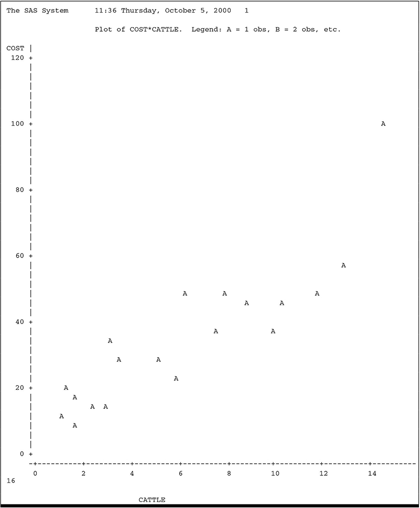
Output 2.3 is produced by the following statements:
proc reg data=auction;
model cost=cattle;
plot cost*cattle;
run;
The graph shows the values of COST plotted versus CATTLE with the regression plotted through the data. The plot indicates that both assumptions are reasonable, except for the exceptionally large value of COST for CATTLE=14.325.
Output 2.3 Plot of CATTLE Data
2.2.2 The P, CLM, and CLI Options: Predicted Values and Confidence Limits
A common objective of regression analysis is to compute the predicted value
ˆy=ˆβ0+ˆβ1x1+⋯+ˆβkxk
for some selected values of x1, . . . , xk. You can do this in several ways using PROC REG or other regression procedures in SAS. In PROC REG, the most direct way is to use the P (for predicted) option in the MODEL statement. Output 2.4 shows the results from the following SAS statements:
proc reg data=auction;
id cattle;
model cost=cattle / p clm cli;
Output 2.4 PROC REG with the P, CLM, and CLI Options
| The SAS System | 1 | |||||||||
| Dep | Var | Predicted | Std Err | |||||||
| Obs | CATTLE | COST | Value | Mean | Predict | 95% | CL Mean | |||
| 1 | 3.437 | 27.6980 | 22.8828 | 2.9041 | 16.7558 | 29.0099 | ||||
| 2 | 12.801 | 57.6340 | 65.6197 | 4.6192 | 55.8741 | 75.3653 | ||||
| 3 | 6.136 | 47.1720 | 35.2009 | 2.4162 | 30.1031 | 40.2987 | ||||
| 4 | 11.685 | 49.2950 | 60.5263 | 4.0704 | 51.9386 | 69.1140 | ||||
| 5 | 5.733 | 24.1150 | 33.3617 | 2.4292 | 28.2365 | 38.4868 | ||||
| 6 | 3.021 | 33.6120 | 20.9842 | 3.0477 | 14.5541 | 27.4143 | ||||
| 7 | 1.689 | 9.5120 | 14.9050 | 3.5837 | 7.3440 | 22.4661 | ||||
| 8 | 2.339 | 14.7550 | 17.8716 | 3.3095 | 10.8891 | 24.8541 | ||||
| 9 | 1.025 | 10.5700 | 11.8746 | 3.8834 | 3.6814 | 20.0677 | ||||
| 10 | 2.936 | 15.3940 | 20.5963 | 3.0787 | 14.1009 | 27.0917 | ||||
| 11 | 5.049 | 27.8430 | 30.2399 | 2.5037 | 24.9576 | 35.5222 | ||||
| 12 | 1.693 | 17.7170 | 14.9233 | 3.5820 | 7.3659 | 22.4806 | ||||
| 13 | 1.187 | 20.2530 | 12.6139 | 3.8087 | 4.5783 | 20.6496 | ||||
| 14 | 9.730 | 37.4650 | 51.6038 | 3.2127 | 44.8257 | 58.3819 | ||||
| 15 | 14.325 | 101.3340 | 72.5752 | 5.4094 | 61.1624 | 83.9880 | ||||
| 16 | 7.737 | 47.4270 | 42.5078 | 2.5914 | 37.0405 | 47.9751 | ||||
| 17 | 7.538 | 35.9440 | 41.5996 | 2.5511 | 36.2172 | 46.9820 | ||||
| 18 | 10.211 | 45.9450 | 53.7991 | 3.4072 | 46.6104 | 60.9877 | ||||
| 19 | 8.697 | 46.8900 | 46.8892 | 2.8468 | 40.8831 | 52.8954 | ||||
| Obs | CATTLE | 95% | CL | Predict | Residual | ||||
| 1 | 3.437 | -0.1670 | 45.9326 | 4.8152 | |||||
| 2 | 12.801 | 41.3560 | 89.8834 | -7.9857 | |||||
| 3 | 6.136 | 12.4031 | 57.9987 | 11.9711 | |||||
| 4 | 11.685 | 36.7041 | 84.3486 | -11.2313 | |||||
| 5 | 5.733 | 10.5577 | 56.1656 | -9.2467 | |||||
| 6 | 3.021 | -2.1480 | 44.1164 | 12.6278 | |||||
| 7 | 1.689 | -8.5667 | 38.3767 | -5.3930 | |||||
| 8 | 2.339 | -5.4202 | 41.1634 | -3.1166 | |||||
| 9 | 1.025 | -11.8083 | 35.5575 | -1.3046 | |||||
| 10 | 2.936 | -2.5542 | 43.7467 | -5.2023 | |||||
| 11 | 5.049 | 7.4002 | 53.0797 | -2.3969 | |||||
| 12 | 1.693 | -8.5472 | 38.3938 | 2.7937 | |||||
| 13 | 1.187 | -11.0149 | 36.2428 | 7.6391 | |||||
| 14 | 9.730 | 28.3725 | 74.8351 | -14.1388 | |||||
| 15 | 14.325 | 47.5951 | 97.5552 | 28.7588 | |||||
| 16 | 7.737 | 19.6246 | 65.3911 | 4.9192 | |||||
| 17 | 7.538 | 18.7365 | 64.4627 | -5.6556 | |||||
| 18 | 10.211 | 30.4447 | 77.1535 | -7.8541 | |||||
| 19 | 8.697 | 23.8713 | 69.9072 | 0.0008 | |||||
Specifying the P option in the MODEL statement causes PROC REG to compute predicted values corresponding to each observation in the data set. These computations are printed following the basic PROC REG output under the heading Predict Value. The P option also causes the observed y values (in this case COST) to be printed under the heading Dep Var COST, along with the residuals, where Residual = Dep Var COST – Predict Value.
The estimated standard errors of the predicted values are also printed as a result of the P option. These are computed according to the formula Std Err Predict =√V(ˆy)
The ID statement identifies each observation according to the value of the variable indicated in the statement; in this case CATTLE. This enables you to relate the observed and predicted values to the values of another variable. Usually, one of the independent variables is the most meaningful ID variable.
The CLM option in the MODEL statement gives upper and lower 95% confidence limits for the mean of the subpopulation corresponding to specific values of the independent variables. The CLM option makes the following computation:
(ˆy − tα/2(STD ERR PREDICT) , ˆy + tα/2(STD ERR PREDICT))
The CLI option in the MODEL statement gives upper and lower 95% prediction intervals for a future observation. The CLI option makes the following computation:
(ˆy−ta/2√ˆV(y−ˆy),ˆy+ta/2√ˆV(y−ˆy))
V̂(y − ŷ) is given in Section 2.4.3, with σ2 replaced by MSE.
Consider OBS 4, which has CATTLE=11.685 (see Output 2.5). The observed value of COST for OBS 4 is 49.2950. The predicted value for OBS 4 is 60.5263 (see Output 2.4). This number is used to estimate the expected cost of operation corresponding to CATTLE=11.685, computed as 60.526 = 7.196 + 4.564(11.685). The 95% confidence limits for this mean are (51.9386, 69.1140). The predicted value of 60.5263 is also used to predict COST (not yet observed) of some other randomly drawn auction that has CATTLE=12.685. The 95% prediction limits for this individual sample are (36.7041, 84.3486).
In short, the CLM option yields a confidence interval for the subpopulation mean, and the CLI option yields a prediction interval for a value to be drawn at random from the subpopulation. The CLI limits are always wider than the CLM limits, because the CLM limits accommodate only variability in ŷ whereas the CLI limits accommodate variability in ŷ and variability in the future value of y. This is true even though ŷ is used as an estimate of the subpopulation mean as well as a predictor of the future value.
2.2.3 A Model with Several Independent Variables
This section illustrates regression analyses of data with several independent variables. Output 2.5 shows a data set named AUCTION that has several independent variables.
Output 2.5 Data for Regression with Several Independent Variables
| The SAS System | ||||||||
| OBS | MKT | CATTLE | CALVES | HOGS | SHEEP | COST | VOLUME | TYPE |
| 1 | 1 | 3.437 | 5.791 | 3.268 | 10.649 | 27.698 | 23.145 | O |
| 2 | 2 | 12.801 | 4.558 | 5.751 | 14.375 | 57.634 | 37.485 | O |
| 3 | 3 | 6.136 | 6.223 | 15.175 | 2.811 | 47.172 | 30.345 | O |
| 4 | 4 | 11.685 | 3.212 | 0.639 | 0.694 | 49.295 | 16.230 | B |
| 5 | 5 | 5.733 | 3.220 | 0.534 | 2.052 | 24.115 | 11.539 | B |
| 6 | 6 | 3.021 | 4.348 | 0.839 | 2.356 | 33.612 | 10.564 | B |
| 7 | 7 | 1.689 | 0.634 | 0.318 | 2.209 | 9.512 | 4.850 | O |
| 8 | 8 | 2.339 | 1.895 | 0.610 | 0.605 | 14.755 | 5.449 | B |
| 9 | 9 | 1.025 | 0.834 | 0.734 | 2.825 | 10.570 | 5.418 | O |
| 10 | 10 | 2.936 | 1.419 | 0.331 | 0.231 | 15.394 | 4.917 | B |
| 11 | 11 | 5.049 | 4.195 | 1.589 | 1.957 | 27.843 | 12.790 | B |
| 12 | 12 | 1.693 | 3.602 | 0.837 | 1.582 | 17.717 | 7.714 | B |
| 13 | 13 | 1.187 | 2.679 | 0.459 | 18.837 | 20.253 | 23.162 | O |
| 14 | 14 | 9.730 | 3.951 | 3.780 | 0.524 | 37.465 | 17.985 | B |
| 15 | 15 | 14.325 | 4.300 | 10.781 | 36.863 | 101.334 | 66.269 | O |
| 16 | 16 | 7.737 | 9.043 | 1.394 | 1.524 | 47.427 | 19.698 | B |
| 17 | 17 | 7.538 | 4.538 | 2.565 | 5.109 | 35.944 | 19.750 | B |
| 18 | 18 | 10.211 | 4.994 | 3.081 | 3.681 | 45.945 | 21.967 | B |
| 19 | 19 | 8.697 | 3.005 | 1.378 | 3.338 | 46.890 | 16.418 | B |
The AUCTION data set is an expansion of the MARKET data set. It contains data from the 19 livestock auction markets for sales of four classes of livestock—CATTLE, CALVES, HOGS, and SHEEP. The objective is to relate the annual cost (in thousands of dollars) of operating a livestock market (COST) to the number (in thousands) of livestock in various classes (CATTLE, CALVES, HOGS, SHEEP) that were sold in each market. This is done with a multiple regression analysis. The variables VOLUME and TYPE are used later.
The multiple regression model
COST = β0 + β1 CATTLE + β2 CALVES + β3 HOGS + β4 SHEEP + ε (2.4)
relates COST to the four predictor variables. To fit this model, use the following SAS statements:
proc reg;
model cost=cattle calves hogs sheep;
The results appear in Output 2.6.
Output 2.6 Results for Regression with Several Independent Variables
| The SAS System | 1 | |
| Model: MODEL1 | ||
| Dependent variable: COST | ||
| Analysis of Variance | |||||||||
| Sum of | Mean | ||||||||
| Source | DF | Squares | Square | ➊ | F Value | ➋ | Prob>F | ||
| Model | 4 | 7936.73649 | 1984.18412 | 52.610 | 0.0001 | ||||
| Error | 14 | 531.03865 | 37.93133 | ||||||
| C Total | 18 | 8467.77514 | |||||||
| Root MSE | 6.15884 | ➌ | R-square | 0.9373 |
| Dep Mean | 35.29342 | ➍ | Adj R-sq | 0.9194 |
| C.V. | 17.45040 | |||
| Parameter Estimates | |||||||||
| ➎ | Parameter | ➏ | Standard | ➐ | T for H0: | ||||
| Variable | DF | Estimate | Error | Parameter=0 | ➑ | Prob > |T| | |||
| INTERCEP | 1 | 2.288425 | 3.38737222 | 0.676 | 0.5103 | ||||
| CATTLE | 1 | 3.215525 | 0.42215239 | 7.616 | 0.0001 | ||||
| CALVES | 1 | 1.613148 | 0.85167539 | 1.894 | 0.0791 | ||||
| HOGS | 1 | 0.814849 | 0.47073855 | 1.737 | 0.1054 | ||||
| SHEEP | 1 | 0.802579 | 0.18981766 | 4.228 | 0.0008 | ||||
The upper portion of the output, as in Output 2.2, contains the partitioning of TOTAL SS, labeled C Total, into MODEL SS and ERROR SS, along with the corresponding mean squares. The callout numbers have been added to the output to key the descriptions that follow:
➊ The F-value of 52.610 is used to test the null hypothesis
H0 : β1 = β2 = β3 = β4 = 0
➋ The associated p-value (Prob>F) of 0.0001 leads to a rejection of this hypothesis and to the conclusion that some of the β's are not 0.
➌ R-square=0.9373 shows that a large portion of the variation in COST can be explained by variation in the independent variables in the model.
➍ Adj R-sq=0.9194 is an alternative to R-square that is adjusted for the number of parameters in the model according to the formula
ADJ R-SQ = 1 - (1 − R-SQUARE)((n − 1) / (n − m − 1))
where n is the number of observations in the data set and m is the number of regression parameters in the model, excluding the intercept. This adjustment is used to overcome an objection to R-square as a measure of goodness of fit of the model. This objection stems from the fact that R-square can be driven to 1 simply by adding superfluous variables to the model with no real improvement in fit. This is not the case with Adj R-sq, which tends to stabilize to a certain value when an adequate set of variables is included in the model.
➎ The Parameter Estimates give the fitted model
^COST=2.29+3.22(CATTLE)+1.61(CALVES)+0.81(HOGS) +0.80(SHEEP)
Thus, for example, one head of CATTLE contributes $3.22 to the COST of operating a market, if all other numbers of livestock are held fixed. Remember that the COST of operating the markets was given in $1000 units, whereas the numbers of animals were given in 1000-head units.
➏ These are the (estimated) Standard Errors of the parameter estimates and are useful for constructing confidence intervals for the parameters, as shown in Section 2.4.3.
➐ The t-tests (T for H0 : Parameter=0) are used for testing hypotheses about individual parameters. It is important that you clearly understand the interpretation of these tests. This can be explained in terms of comparing the fits of complete and reduced models. (Review Section 2.4.2, “Partitioning the Sums of Squares.”) The complete model for all of these t-tests contains all the variables on the right-hand side of the MODEL statement. The reduced model for a particular test contains all these variables except the one being tested. Thus, the t-statistic=1.894 for testing the hypothesis H0 : β2 = 0 is actually testing whether the complete model containing CATTLE, CALVES, HOGS, and SHEEP fits better than the reduced model containing only CATTLE, HOGS, and SHEEP.
➑ The p-value (Prob > | T |) for this test is p=0.0791.
2.2.4 The SS1 and SS2 Options: Two Types of Sums of Squares
PROC REG can compute two types of sums of squares associated with the estimated coefficients in the model. These are referred to as Type I and Type II sums of squares and are computed by specifying SS1 or SS2, or both, as MODEL statement options. For example, the following SAS statements produce Output 2.7:
proc reg;
model cost=cattle calves hogs sheep / ss1 ss2;
run;
Output 2.7 PROC REG with the SS1 and SS2 MODEL Statement Options
| The SAS System | ||
| Model: MODEL1 | ||
| Dependent variable: COST | ||
| Analysis of Variance | |||||||||
| Sum of | Mean | ||||||||
| Source | DF | Squares | Square | F Value | Prob>F | ||||
| Model | 4 | 7936.73649 | 1984.18412 | 52.610 | 0.0001 | ||||
| Error | 14 | 531.03865 | 37.93133 | ||||||
| C Total | 18 | 8467.77514 | |||||||
| Root MSE | 6.15884 | R-square | 0.9373 | |
| Dep Mean | 35.29342 | Adj R-sq | 0.9194 | |
| C.V. | 17.45040 | |||
| Parameter Estimates | |||||||||
| Parameter | Standard | T for H0: | |||||||
| Variable | DF | Estimate | Error | Parameter=0 | Prob > |T| | ||||
| INTERCEP | 1 | 2.288425 | 3.38737222 | 0.676 | 0.5103 | ||||
| CATTLE | 1 | 3.215525 | 0.42215239 | 7.616 | 0.0001 | ||||
| CALVES | 1 | 1.613148 | 0.85167539 | 1.894 | 0.0791 | ||||
| HOGS | 1 | 0.814849 | 0.47073855 | 1.737 | 0.1054 | ||||
| SHEEP | 1 | 0.802579 | 0.18981766 | 4.228 | 0.0008 | ||||
| Variable | DF | Type I SS | Type II SS | ||||||
| INTERCEP | 1 | 23667 | 17.311929 | ||||||
| CATTLE | 1 | 6582.091806 | 2200.712494 | ||||||
| CALVES | 1 | 186.671101 | 136.081196 | ||||||
| HOGS | 1 | 489.863790 | 113.656260 | ||||||
| SHEEP | 1 | 678.109792 | 678.109792 | ||||||
These sums of squares are printed as additional columns and are labeled Type I SS and Type II SS. You may find it helpful at this point to review the material in Section 2.4. In particular, the concepts of partitioning sums of squares, complete and reduced models, and reduction notation are useful in understanding the different types of sums of squares.
The Type I SS are commonly called sequential sums of squares. They represent a partitioning of the MODEL SS into component sums of squares due to adding each variable sequentially to the model in the order prescribed by the MODEL statement.
The Type I SS for the INTERCEP is simply ny̅2. It is called the correction for the mean. The Type I SS for CATTLE (6582.09181) is the MODEL SS for a regression equation that contains only CATTLE. The Type I SS for CALVES (186.67110) is the increase in MODEL SS due to adding CALVES to the model that already contains CATTLE. In general, the Type I SS for a particular variable is the sum of squares due to adding that variable to a model that already contains all the variables that preceded the particular variable in the MODEL statement. Continuing the pattern, you see that the Type I SS for HOGS (489.86379) is the increase in MODEL SS due to adding HOGS to a model that already contains CATTLE and CALVES. Finally, the Type I SS for SHEEP (678.10979) is the increase in MODEL SS due to adding SHEEP to a model that already contains CATTLE, CALVES, and HOGS. Note that
MODEL SS = 7936.7 = 6582.1 + 186.7 + 489.9 + 678.1
illustrates the sequential partitioning of the MODEL SS into the Type I components that correspond to the variables in the model.
The Type II SS are commonly called the partial sums of squares. For a given variable, the Type II SS is equivalent to the Type I SS for that variable if it were the last variable in the MODEL statement. (Note that the Type I SS and Type II SS for SHEEP are equal in Output 2.7.) In other words, the Type II SS for a particular variable is the increase in MODEL SS due to adding the variable to a model that already contains all the other variables in the MODEL statement. The Type II SS, therefore, do not depend on the order in which the independent variables are listed in the MODEL statement. Furthermore, they do not yield a partitioning of the MODEL SS unless the independent variables are uncorrelated.
The Type I SS and Type II SS are shown in the table below in reduction notation (see Section 2.4.2):
| Type I (Sequential) |
Type II (Partial) |
|
|---|---|---|
| CATTLE | R(β1 | β0) | R(β1 | β0, β2, β3, β4) |
| CALVES | R(β2| β0, β1) | R(β2| β0, β1, β3, β4) |
| HOGS | R(β3| β0, β1, β2) | R(β3| β0, β1, β2, β4) |
| SHEEP | R(β4| β0, β1, β2, β3) | R(β4| β0, β1, β2, β3) |
The reduction notation provides a convenient device to determine the complete and reduced models that are compared if you construct an F-test using one of these sums of squares. First, note that each sum of squares for a particular variable has one degree of freedom, so that the sums of squares are also mean squares. Thus, for example, a Type I F-test for CALVES is given by
F = Type I SS for CALVESMSE = 186.737.9 = 4.92
The reduction notation shows that this F-value would be used to test whether the complete model containing CATTLE and CALVES fits the data significantly better than the reduced model containing only CATTLE. Similarly, a Type II F-statistic for CALVES is given by
F = Type II SS for CALVESMSE = 136.137.9 = 3.59
It would be used to test whether the complete model containing CATTLE, CALVES, HOGS, and SHEEP fits significantly better than the reduced model containing CATTLE, HOGS, and SHEEP. In this example, the difference between these two F-values is not great. The difference between Type I and Type II F-values for HOGS is considerably greater. The variation due to HOGS that is not due to CATTLE and CALVES is 489.86379, but the variation due to HOGS that is not due to CATTLE, CALVES, and SHEEP is only 113.65626. The former is significant at the 0.003 level, whereas the latter is significant only at the 0.105 level. Thus, a model containing CATTLE and CALVES is significantly improved by adding HOGS, but a model containing CATTLE, CALVES, and SHEEP is improved much less by adding HOGS.
PROC REG does not compute F-values for the Type I and Type II sums of squares, nor does it compute the corresponding significance probabilities. However, you can use PROC GLM to make the same computations discussed in this chapter. There are several other distinctions between the capabilities of PROC REG and PROC GLM. Not all analyses using PROC REG can be easily performed by PROC GLM. Some of these distinctions are discussed in subsequent sections.
It is now appropriate to note that the Type II F-tests are exactly equivalent to the t-tests for the parameters because they are comparing the same complete and reduced models. In fact, the Type II F-statistic for a given variable is equal to the square of the t-statistic for the same variable.
For most applications, the desired test for a single parameter is based on the Type II sums of squares, which are equivalent to the t-tests for the parameter estimates. Type I sums of squares, however, are useful if there is need for a specific sequencing of tests on individual coefficients as, for example, in polynomial models.
2.2.5 Tests of Subsets and Linear Combinations of Coefficients
Tests of hypotheses that individual coefficients are equal to 0 are given by the t-tests on the parameters in the basic PROC REG output, as discussed in Section 2.2.3. In this section, a direct procedure is demonstrated for testing that subsets of coefficients are equal to 0. These tests are specified in the optional TEST statement in PROC REG. The TEST statement can also be used to test that linear functions of parameters are equal to specified constants.
The TEST statement must follow a MODEL statement in PROC REG. Several TEST statements can follow one MODEL statement. The general form of the TEST statement is
label: TEST equation <, . . . , equation>< / option>;
The label is optional and serves only to identify results in the output. The equations provide the technical information that PROC REG uses to determine what hypotheses are to be tested. These tests can be interpreted in terms of comparing complete and reduced (or restricted) models in the same manner as discussed in previous sections. The complete model for all tests specified by a TEST statement is the model containing all variables on the right side of the MODEL statement. The reduced model is derived from the complete model by imposing the conditions implied by the equations indicated in the TEST statement.
For illustration, recall the AUCTION data set in Section 2.2.3 and the SAS statement
model cost=cattle calves hogs sheep;
which fits the complete regression model
COST = β0 + β1 (CATTLE) + β2 (CALVES) + β3 (HOGS) + β4 (SHEEP) + ε
To test the hypothesis H0 : β3 = 0, use the statement
hogs: test hogs=0;
This statement tells PROC REG to construct an F-test to compare the complete model with the reduced model
COST = β0 + β1 (CATTLE) + β2 (CALVES) + β4 (SHEEP) + ε
Similarly, to test the hypothesis H0 : β3 = β4 = 0, which is equivalent to H0 : (β3 = 0 and β4 = 0), use the statement
hogsheep: test hogs=0, sheep=0;
The hypothesis of a 0 intercept, is specified with the statement
intercep: test intercept=0;
If the right side of an equation in a TEST statement is 0, you don't need to specify it. PROC REG will assume a right-side value of 0 by default.
More general linear functions are tested in a similar fashion. For example, to test that the average cost of selling one hog is one dollar, you test the hypothesis H0:β3 = 1. This hypothesis is specified in the following TEST statement:
hogone: test hogs=1;
Another possible linear function of interest is to test whether the average cost of selling one hog differs from the average cost of selling one sheep. The null hypothesis is H0:β3 = β4, which is equivalent to H0: β3 − β4 = 0, and is specified by the following statement:
hequals: test hogs-sheep=0;
The results of all five of these TEST statements appear in Output 2.8.
Output 2.8 Results of the TEST Statement
| The SAS System | 1 | ||||||
| Dependent Variable: COST | |||||||
| Test: HOGS | Numerator: | 113.6563 | DF: | 1 | F value: | 2.9964 | |
| Denominator: | 37.93133 | DF: | 14 | Prob>F: | 0.1054 | ||
| Dependent Variable: COST | |||||||
| Test: HOGSHEEP | Numerator: | 583.9868 | DF: | 1 | F value: | 15.3959 | |
| Denominator: | 37.93133 | DF: | 14 | Prob>F: | 0.0003 | ||
| Dependent Variable: COST | |||||||
| Test: INTERCEP | Numerator: | 17.3119 | DF: | 1 | F value: | 0.4564 | |
| Denominator: | 37.93133 | DF: | 14 | Prob>F: | 0.5103 | ||
| Dependent Variable: COST | |||||||
| Test: HOGONE | Numerator: | 5.8680 | DF: | 1 | F value: | 0.1547 | |
| Denominator: | 37.93133 | DF: | 14 | Prob>F: | 0.7000 | ||
| Dependent Variable: COST | |||||||
| Test: HEQUALS | Numerator: | 0.0176 | DF: | 1 | F value: | 0.0005 | |
| Denominator: | 37.93133 | DF: | 14 | Prob>F: | 0.9831 | ||
For each TEST statement indicated, a sum of squares is computed with degrees of freedom equal to the number of equations in the TEST statement. From these quantities, a mean square that forms the numerator of an F-statistic is computed. The denominator of the F-ratio is the mean square for error. The value of F is printed, along with its p-value. The test labeled HOGS is, of course, the equivalent of the t-test for HOGS in Output 2.5.
Note: If there are linear dependencies or inconsistencies among the equations in a TEST statement, then PROC REG prints a message that the test failed, and no F-ratio is computed.
2.2.6 Fitting Restricted Models: The RESTRICT Statement and NOINT Option
Subject to linear restrictions on the parameters, models can be fitted by using the RESTRICT statement in PROC REG. The RESTRICT statement follows a MODEL statement and has the general form
RESTRICT equation <, . . . , equation>;
where each equation is a linear combination of the model parameters set equal to a constant.
Consider again the data set AUCTION and the following MODEL statement:
model cost=cattle calves hogs sheep;
This model is fitted in Section 2.2.3. Inspection of Output 2.5 shows that the INTERCEP estimate is close to 0 and that the parameter estimates for HOGS and SHEEP are similar in value. Hypotheses pertaining to these conditions are tested in Section 2.2.5. The results suggest a model that has 0 intercept and equal coefficients for HOGS and SHEEP, namely
COST=β1(CATTLE)+β2(CALVES)+β(HOGS)+β(SHEEP)+ε
where β is the common value of β3 and β4.
This model can be fitted with the following RESTRICT statement:
restrict intercept=0, hogs-sheep=0;
The results of these statements appear in Output 2.9.
Output 2.9 Results of the RESTRICT Statement
| Model: MODEL1 | ||
| NOTE: Restrictions have been applied to parameter estimates. | ||
| Dependent variable: COST | ||
| Analysis of Variance | |||||||||
| Sum of | Mean | ||||||||
| Source | DF | Squares | Square | F Value | Prob>F | ||||
| Model | 2 | 7918.75621 | 3959.37811 | 115.388 | 0.0001 | ||||
| Error | 16 | 549.01893 | 34.31368 | ||||||
| C Total | 18 | 8467.77514 | |||||||
| Root MSE | 5.85779 | R-square | 0.9352 | |
| Dep Mean | 35.29342 | Adj R-sq | 0.9271 | |
| C.V. | 16.59739 | |||
| Parameter Estimates | |||||||||
| Parameter | Standard | T for H0: | |||||||
| Variable | DF | Estimate | Error | Parameter=0 | Prob > |T| | ||||
| INTERCEP | 1 | 1.110223E–15 | 0.00000000 | ⋅ | ⋅ | ||||
| CATTLE | 1 | 3.300043 | 0.38314175 | 8.613 | 0.0001 | ||||
| CALVES | 1 | 1.943717 | 0.59107649 | 3.328 | 0.0043 | ||||
| HOGS | 1 | 0.806825 | 0.13799841 | 5.847 | 0.0001 | ||||
| SHEEP | 1 | 0.806825 | 0.13799841 | 5.847 | 0.0001 | ||||
| RESTRICT | –1 | 7.905632 | 10..92658296 | 0.724 | 0.4798 | ||||
| RESTRICT | –1 | –9.059424 | 64.91322402 | –0.140 | 0.8907 | ||||
Note that the INTERCEP parameter estimate is 0 (except for round-off error), and the parameter estimates for HOGS and SHEEP have the common value .806825. Note also that there are parameter estimates and associated t-tests for the two equations in the RESTRICT statement. These pertain to the Lagrangian parameters that are incorporated in the restricted minimization of the Error SS.
You will find it useful to compare Output 2.9 with results obtained by invoking the restrictions explicitly. The model with the RESTRICT statement is equivalent to the model
COST = β1(CATTLE) + β2(CALVES) + β(SHEEP + HOGS) + ε
This is a three-variable model with an intercept of 0. The variables are CATTLE, CALVES, and HS, where the variable HS=HOGS + SHEEP. The model is then fitted using PROC REG with the MODEL statement
model cost=cattle calves hs / noint;
where NOINT is the option that specifies that no intercept be included. In other words, the fitted regression plane is forced to pass through the origin. The results appear in Output 2.10, from which the following fitted equation is obtained:
COST = 3.300 (CATTLE) + 1.967(CALVES) + 0.807(HS)
= 3.300 (CATTLE) + 1.967(CALVES) + 0.807(HOGS)
+ 0.807(SHEEP)
Output 2.10 Results of Regression with Implicit Restrictions
| The SAS System | ||
| The REG Procedure | ||
| Model: MODEL1 | ||
| Dependent Variable: cost | ||
| NOTE: No intercept in model. R-Square is redefined. | ||
| Analysis of Variance | |||||||||
| Sum of | Mean | ||||||||
| Source | DF | Squares | Square | F Value | Prob>F | ||||
| Model | 3 | 31586 | 10529 | 306.83 | <.0001 | ||||
| Error | 16 | 549.01893 | 34.31368 | ||||||
| Uncorrected Total | 19 | 32135 | |||||||
| Root MSE | 5.85779 | R-square | 0.9829 | |
| Dep Mean | 35.29342 | Adj R-sq | 0.9797 | |
| Coeff Var | 16.59739 | |||
| Parameter Estimates | |||||||||
| Parameter | Standard | ||||||||
| Variable | DF | Estimate | Error | t Value | Pr > |t| | ||||
| cattle | 1 | 3.300043 | 0.38314 | 8.61 | <.0001 | ||||
| calves | 1 | 1.96717 | 0.59108 | 3.33 | 0.0043 | ||||
| hs | 1 | 0.80682 | 0.13800 | 5.85 | <.0001 | ||||
This is the same fitted model obtained in Output 2.9 by using the RESTRICT statements.
As just pointed out, equivalent restrictions can be imposed in different ways using PROC REG. When the NOINT option is used to restrict β0 to be 0, however, caution is advised in trying to interpret the sums of squares, F-values, and R-squares. Notice, for instance, that the MODEL SS do not agree in Output 2.9 and Output 2.10. The ERROR SS and degrees of freedom do agree. In Output 2.9, the MODEL SS and ERROR SS sum to the Corrected Total SS (C Total), whereas in Output 2.10 they sum to the Uncorrected Total SS (U Total). In Output 2.10, the MODEL F-statistic is testing whether the fitted model fits better than a model containing no parameters, a test that has little or no practical value.
Corresponding complications arise regarding the R-square statistic with no-intercept models. Note that R-Square=0.9829 for the no-intercept model in Output 2.10 is greater than R-Square=0.9373 for the model in Output 2.6, although the latter has two more parameters than the former. This seems contrary to the general phenomenon that adding terms to a model causes the R-square to increase. This seeming contradiction occurs because the denominator of the R-square is the Uncorrected Total SS when the NOINT option is used. This is the reason for the message that R-square is redefined at the top of Output 2.10. It is, therefore, not meaningful to compare an R-square for a model that contains an intercept with an R-square for a model that does not contain an intercept.
2.2.7 Exact Linear Dependency
Linear dependency occurs when exact linear relationships exist among the independent variables, that is, when one or more of the columns of the X matrix (see Section 2.4) can be expressed as a linear combination of the other columns. In this event, the X'X matrix is singular and cannot be inverted in the usual sense to obtain parameter estimates. If this occurs, PROC REG uses a generalized inverse to compute parameter estimates. However, care must be exercised to determine exactly what parameters are being estimated. More technically, the generalized inverse approach yields one particular solution to the normal equations. The PROC REG computations are illustrated with the auction market data.
Recall the variable VOLUME in Output 2.5. VOLUME represents the total of all major livestock sold in each market. This is an example of exact linear dependency: VOLUME is exactly the sum of the variables CATTLE, CALVES, HOGS, and SHEEP.
The following statements produce the results shown in Output 2.11:
proc reg;
model cost=cattle calves hogs sheep volume;
Output 2.11 Results of Exact Collinearity
| NOTE: Model is not full rank. Least-squares solutions for the parameters are not unique. Some statistics will be misleading. A reported DF of 0 or B means that the estimate is biased. | ||
| NOTE: The following parameters have been set to 0, since the variables are a linear combination of other variables as shown. | ||
| VOLUME = CATTLE + CALVES + HOGS + SHEEP Parameter Estimates |
| Parameter | Standard | ||||||||
| Variable | DF | Estimate | Error | t Value | Pr > |t| | ||||
| Intercept | 1 | 2.28842 | 3.38737 | 0.68 | 0.5103 | ||||
| CATTLE | B | 3.21552 | 0.42215 | 7.62 | <.0001 | ||||
| CALVES | B | 1.61315 | 0.85168 | 1.89 | 0.0791 | ||||
| HOGS | B | 0.81485 | 0.47074 | 1.73 | 0.1054 | ||||
| SHEEP | B | 0.80258 | 0.18982 | 4.23 | 0.0008 | ||||
| VOLUME | 0 | 0 | ⋅ | ⋅ | ⋅ | ||||
In Output 2.11, the existence of the collinearity is indicated by the notes in the model summary, followed by the equation describing the collinearity. The parameter estimates that are printed are equivalent to the ones that are obtained if VOLUME were not included in the MODEL statement. A variable that is a linear combination of other variables that precede it in the MODEL statement is indicated by 0 under the DF and Parameter Estimate headings. Other variables involved in the linear dependencies are indicated with a B, for bias, under the DF heading. The estimates are, in fact, unbiased estimates of the parameters in a model that does not include the variables indicated with a 0 but are biased for the parameters in the other models. Thus, the parameter estimates printed in Output 2.11 are unbiased estimates for the coefficients in the model
COST = β0 + β1(CATTLE) + β2 (CALVES) + β3 (HOGS)
+ β4(SHEEP) + ε
But these estimates are biased for the parameters in a model that included VOLUME but did not include, for example, SHEEP.
2.3 The GLM Procedure
The REG procedure was used in Section 2.2 to introduce simple and multiple linear regression. In this section, PROC GLM will be used to obtain some of the same analyses you saw in Section 2.2. The purpose is to provide a springboard from which to launch the linear model analysis methodology that will be used throughout the remainder of this book. The basic syntax of PROC GLM is very similar to that of PROC REG for fitting linear regression models. Beyond the basic applications the two procedures become more specialized in their capabilities. PROC REG has greater regression diagnostic and graphic features, but PROC GLM has the ability to create “dummy” variables. This makes PROC GLM suited for analysis of variance, analysis of covariance, and certain mixed-model applications.
The following SAS statements invoke PROC GLM:
proc glm;
model list-of-dependent-variables=list-of-independent-variables;
Options on the PROC, MODEL, and other statements permit specialized and customized analyses.
2.3.1 Using the GLM Procedure to Fit a Linear Regression Model
PROC GLM can fit linear regression models and compute essentially the same basic statistics as PROC REG. These statements apply PROC GLM to fit a multiple linear regression model to the AUCTION data. Results appear in Output 2.12.
proc glm;
model cost=cattle calves hogs sheep;
run;
Output 2.12 Results Using PROC GLM for Multiple Linear Regression
| The SAS System | ||
| The GLM Procedure | ||
| Number of observations 19 | ||
| The SAS System | ||
| The GLM Procedure | ||
| Dependent Variable: COST | ||
| Sum of | ||||||
| Source | DF | Squares | Mean Square | F Value | Pr > F | |
| Model | 4 | 7936.736489 | 1984.184122 | 52.31 | <.0001 | |
| Error | 14 | 531.038650 | 37.931332 | |||
| Corrected Total | 18 | 8467.775139 | ||||
| R-Square | Coeff Var | Root MSE | COST Mean |
| 0.937287 | 17.45040 | 6.158842 | 35.29342 |
| Source | DF | Type I SS | Mean Square | F Value | Pr > F |
| CATTLE | 1 | 6582.091806 | 6582.091806 | 173.53 | <.0001 |
| CALVES | 1 | 186.671101 | 186.671101 | 4.92 | 0.0436 |
| HOGS | 1 | 489.863790 | 489.863790 | 12.91 | 0.0029 |
| SHEEP | 1 | 678.109792 | 678.109792 | 17.88 | 0.0008 |
| Source | DF | Type III SS | Mean Square | F Value | Pr > F |
| CATTLE | 1 | 2200.712494 | 2200.712494 | 58.02 | <.0001 |
| CALVES | 1 | 136.081196 | 136.081196 | 3.59 | 0.0791 |
| HOGS | 1 | 113.656260 | 113.656260 | 3.00 | 0.1054 |
| SHEEP | 1 | 678.109792 | 678.109792 | 17.88 | 0.0008 |
| Standard | ||||
| Parameter | Estimate | Error | t Value | Pr > |t| |
| Intercept | 2.288424577 | 3.38737222 | 0.68 | 0.5103 |
| CATTLE | 3.215524803 | 0.42215239 | 7.62 | <.0001 |
| CALVES | 1.613147614 | 0.85167539 | 1.89 | 0.0791 |
| HOGS | 0.814849491 | 0.47073855 | 1.73 | 0.1054 |
| SHEEP | 0.802578622 | 0.18981766 | 4.23 | 0.0008 |
Compare Output 2.12 with Output 2.6. You find the same partition of sums of squares, with slightly different labels. You also find the same R-square, Root MSE, F-test for the Model, and other statistics. In addition, you find the same parameter estimates for the fitted model, giving the regression equation
COST = 2.288 + 3.215 CATTLE + 1.612 CALVES + 0.815 HOGS + 0.803 SHEEP
Compare Output 2.12 with Output 2.7. You see that the Type I sums of squares are the same from PROC GLM and PROC REG. You also see that the Type III sums of squares from GLM are the same as the Type II sums of squares from PROC REG. In fact, there are also Types II and IV sums of squares available from PROC GLM whose values would be the same as the Type II sums of squares from PROC REG. In general, Types II, III, and IV sums of squares are identical for regression models, but differ for some ANOVA models, as you will see in subsequent chapters.
2.3.2 Using the CONTRAST Statement to Test Hypotheses about Regression Parameters
Fitting a regression model is just one step in a regression analysis. You usually want to do more analyses to answer specific questions about the variables in the model. In Section 2.2.3 you learned how to test the hypothesis
H0 : β1 = β2 = β3 = β4 = 0
using the test statistic F = MS Model / MS Error. You also learned how to test the hypotheses of individual parameters. For example, the hypothesis that the CALVES parameter is zero,
H0 : β2 = 0
can be tested using t-statistics for the parameter estimates. In Section 2.2.4, you learned how to test the hypothesis
H0 : β2 = 0
using an F-statistic based on either the Type I or the Type II sum of squares. Output 2.12 shows the F-values of 4.92 based on the Type I sum of squares, and 3.59 based on the Type III (= Type II) sum of squares. These F-values have p-values of 0.0436 and 0.0791. These are different because the reference models are different for the hypotheses. The distinction is even more dramatic for hypotheses about the SHEEP regression parameter, β3. The Type I F-test for H0 : β3 = 0 has p-value of 0.0029, and the Type III F-test for H0 : β3 = 0 has p-value of 0.1054.
You can test a hypothesis of the form
H0 : β1 = β2 = 0
in the reference model COST = β0 + β1 CATTLE + β2 CALVES + β3 +HOGS + ε using the F-statistic
F = MS(β1, β2 | β0, β3) / MS(ERROR),
where MS(β1, β2 | β0, β3) = R(β1, β2 | β0, β3) / 2, and
R(β1, β2 | β0, β3) = R(β1 | β0) + R(β2 | β0, β1).
These computations can be obtained by using Type I sums of squares:
MS(β1, β2 | β0, β3) = (2200.71 + 136.08)/2
= 1168.40,
and thus F = 1168.40/37.93 = 30.80. The p-value for F = 30.80 is <.0001.
Other hypotheses about regression parameters can be tested using a special tool in PROC GLM called CONTRAST statements. CONTRAST statements can be used to test hypotheses about any linear combination of parameters in the model.
Next you will see how to test the following hypotheses using the CONTRAST statement:
| ❏ | H0 : β3 = 0 | (Cost of HOGS is zero) |
| ❏ | H0 : β3 = β4 | (Cost of HOGS is equal to cost of SHEEP) |
| ❏ | H0 : β3 = β4 = 0 | (Costs of HOGS and SHEEP are both equal to zero) |
The basic syntax of the CONTRAST statement is
contrast ‘label’ effect values;
where effect values refers to coefficients of a linear combination of parameters, and label simply refers to a character string to identify the results in the PROC GLM output. For our regression example, a hypothesis about a linear combination of parameters would have the form
H0 : a0 β0 + a1 β1 + a2 β2 + a3 β3 + a4 β4 = 0
where a0, a1, a2, a3, and a4 are numbers. This hypothesis would be indicated in a CONTRAST statement as
contrast ‘label’ intercept a0 cattle a1 calves a2 hogs a3 sheep a4;
The linear combination in the hypothesis H0 : β3 = 0 is simply β3, so a3 = 1 and a0, a1, a2, and a4 and are all equal to zero. Therefore, you could use the CONTRAST statement
contrast ‘hogcost=0’ intercept 0 cattle 0 calves 0 hogs 1 sheep 0;
Actually, you only need to specify the nonzero constants. Others will be set to zero implicitly. So you could write the CONTRAST statement to test the hypothesis H0 : β3 = 0 as
contrast ‘hogcost=0’ hogs 1;
You can follow the same logic and get a test of the hypothesis H0 : β3 = β4. Write this hypothesis as H0 : β3 – β4 = 0. The linear combination you are testing is β3 – β4, so a3 =1 and a4 = –1, and the other constants are zero. This leads to the CONTRAST statement
contrast ‘hogcost=sheepcost’ hogs 1 sheep –1;
The third hypothesis H0 : β3 = β4 = 0 is different from the first two because it entails two linear combinations simultaneously. Actually, the hypothesis should be written
H0 : β3 = 0 and β4 = 0
Then you see that the two linear combinations are β3 and β4. You can specify two or more linear combinations in a CONTRAST statement by separating their coefficients with commas. A CONTRAST statement to test this hypothesis is
contrast ‘hogcost=sheepcost=0’ hogs 1, sheep 1;
Now run the statements
proc glm;
model cost=cattle calves hogs sheep;
contrast ‘hogcost=0’ hogs 1;
contrast ‘hogcost=sheepcost’ hogs 1 sheep -1;
contrast ‘hogcost=sheepcost=0’ hogs 1, sheep 1;
run;
Results of the CONTRAST statements appear in Output 2.13.
Output 2.13 Results from the CONTRAST Statements in Multiple Linear Regression
| Contrast | DF | Contrast SS | Mean Square | F Value | Pr < F |
| hogcost=0 | 1 | 113.656260 | 113.656260 | 3.00 | 0.1054 |
| hogcost=sheepcost | 1 | 0.017568 | 0.017568 | 0.00 | 0.9831 |
| hogcost=sheepcost=0 | 2 | 1167.973582 | 583.986791 | 15.40 | 0.0003 |
2.3.3 Using the ESTIMATE Statement to Estimate Linear Combinations of Parameters
You learned how to test hypotheses about linear combinations of parameters using the CONTRAST statement in Section 2.3.2. Sometimes it is more meaningful to estimate the linear combinations. You can do this with the ESTIMATE statement in PROC GLM. The ESTIMATE statement is used in essentially the same way as the CONTRAST statement. But instead of F-tests for linear combinations, you get estimates of them along with standard errors. However, the ESTIMATE statement can estimate only one linear combination at a time, whereas the CONTRAST statement could be used to test two or more linear combinations simultaneously.
Consider the first two linear combinations you tested in Section 2.3.2, namely β3 and β3 – β4. You can estimate these linear combinations by using the ESTIMATE statements
estimate ‘hogcost=0’ hogs 1;
estimate ‘hogcost=sheepcost’ hogs 1 sheep -1;
Results are shown in Output 2.14.
Output 2.14 Results from the ESTIMATE Statements in Multiple Linear Regression
| Standard | ||||
| Parameter | Estimate | Error | t Value | Pr > |t| |
| hogcost-sheepcost | 0.0122709 | 0.57018280 | 0.02 | 0.9831 |
| cost predict | 24.7405214 | 1.75311927 | 14.11 | <.0001 |
Compare Output 2.14 with Output 2.13. You see that the F-values in Output 2.13 are equal to the squares of the t-values in Output 2.14. Therefore, they are equivalent test statistics. You can confirm this by noting that the F-tests in Output 2.13 have the same p-values as the t-tests in Output 2.14. The advantage of the ESTIMATE statement is that it gives you estimates of the linear combinations and standard errors in addition to the tests of significance.
2.4 Statistical Background
The REG and GLM procedures implement a multiple linear regression analysis according to the model
y = β0 + β1x1 + β2x2 +…+ βmxm + ε
which relates the behavior of a dependent variable y to a linear function of the set of independent variables x1, x2, …, xm. The βi’s are the parameters that specify the nature of the relationship, and ε is the random error term. Although it is assumed that you have a basic understanding of regression analysis, it may be helpful to review regression principles, terminology, notation, and procedures.
2.4.1 Terminology and Notation
The principle of least squares is applied to a set of n observed values of y and the associated values of xi to obtain estimates ˆβ0,ˆβ1,…,ˆβm
ˆy = ˆβ0 + ˆβ1x1 + . . . + ˆβmxm
Many regression computations are illustrated conveniently in matrix notation. Letting yj, xij, and εj denote the values of y, xi, and ε, respectively, in the jth observation, the Y vector, the X matrix, and the ε vector can be defined as
y11x11...xm1ε1.....Y=.X=...ε=......yn1x1n...xmnεn
Then the model in matrix notation is
Y = Xβ + ε
where β′ = (β0, β1,...,βm) is the parameter vector.
The vector of least-squares estimates, ˆβ′=(ˆβ0, ˆβ1, . . . , ˆβm),
X′Xˆβ = X′Y
Assuming that X'X has full rank, there is a unique solution to the normal equations given by
ˆβ = (X′X)−1X′Y
The matrix (X′X)−1 is useful in regression analysis and is often denoted by
(X′X)−1 = C = [c00c01. . .c0mc10c11. . .c1m.........cm0cm1. . .cmm]
The C matrix provides the variances and covariances of the regression parameter estimates V(β̂) = σ2C, where σ2 = V (εi).
2.4.2 Partitioning the Sums of Squares
A basic identity results from least squares, specifically,
∑(y−ˉy)2=∑(ˆy−ˉy)2+∑(y−ˆy)2
This identity shows that the total sum of squared deviations from the mean, Σ(y − y̅)2, can be partitioned into two parts: the sum of squared deviations from the regression line to the overall mean, Σ(ˆy−ˉy)2
TOTAL SS = MODEL SS + ERROR SS
The TOTAL SS always has the same value for a given set of data, regardless of the model that is fitted. However, partitioning into MODEL SS and ERROR SS depends on the model. Generally, the addition of a new x variable to a model will increase the MODEL SS and, correspondingly, reduce the RESIDUAL SS. In matrix notation, the residual or error sum of squares is
ERRORSS=Y′(I−X(X′X)−1X′)Y=Y′Y−Y′X(X′X)−1X′Y=Y′Y−ˆβX′Y
The error mean square
s2 = MSE = ERROR SS / (n − m − 1)
is an unbiased estimate of σ2, the variance of εi.
PROC REG and PROC GLM compute several sums of squares. Each sum of squares can be expressed as the difference between the regression sums of squares for two models, which are called complete and reduced models. This approach relates a given sum of squares to the comparison of two regression models.
Denote by MODEL SS1 the MODEL SS for a regression with m = 5 x variables:
y = β0 + β1x1 + β2x2 + β3x3 + β4x4 + β5x5 + ε
and by MODEL SS2 the MODEL SS for a reduced model not containing x4 and x5:
y = β0 + β1x1 + β2x2 + β3x3 + ε
Reduction in sum of squares notation can be used to represent the difference between regression sums of squares for the two models. For example,
R(β4, β5 | β0, β1, β2, β3) = MODEL SS1 − MODEL SS2
The difference, or reduction in error, R(β4, β5 | β0, β1, β2, β3) indicates the increase in regression sums of squares due to the addition of β4 and β5 to the reduced model. It follows that
R(β4, β5 | β0, β1, β2, β3) = MODEL SS1 − MODEL SS2
Since TOTAL SS=MODEL SS+ERROR SS, it follows that
R(β4, β5 | β0, β1, β2, β3) = ERROR SS2 − ERROR SS1
The expression R(β4, β5 | β0, β1, β2, β3) is also commonly referred to as
❏ the sum of squares due to β4 and β5 (or x4 and x5) adjusted for β0, β1, β2, β3 (or the intercept and x1, x2, x3)
❏ the sum of squares due to fitting x4 and x5 after fitting the intercept and x1, x2, x3
❏ the effects of x4 and x5 above and beyond, or partial of, the effects of the intercept and x1, x2, x3.
2.4.3 Hypothesis Tests and Confidence Intervals
Inferences about model parameters are highly dependent on the other parameters in the model under consideration. Therefore, in hypothesis testing it is important to emphasize the parameters for which inferences have been adjusted. For example, tests based on R(β3 | β0, β1, β2) and R(β3 | β0, β1) may measure entirely different concepts. Consequently, a test of H0: β3 = 0 versus H0: β3 ≠ 0 may have one result for the model y = β0 + β1x1 + β2x2 + β3x3 + ε and another result for the model y = β0 + β1x1 + β3x3 + ε. Differences reflect relationships among independent variables rather than inconsistencies in statistical methodology.
Statistical inferences can also be made in terms of linear functions of the parameters in the form
H0 : ℓ0β0 + ℓ1β1 +...+ ℓmβm = 0
where the ℓi are constants chosen to correspond to a specified hypothesis. Such functions are estimated by the corresponding linear function
Lˆβ = ℓ0ˆβ0 + ℓ1ˆβ1 + . . . + ℓmˆβm
of the least-squares estimates ˆβ. The variance of Lˆβ is
V(Lˆβ)=(L(X′X)−1L′)σ2
A t-test or F-test is then used to test H0 :(Lβ) = 0. The denominator usually uses the error mean square MSE as the estimate of σ2 Because the variance of the estimated function is based on statistics computed for the entire model, the test of the hypothesis is made in the presence of all model parameters. These tests can be generalized to simultaneous tests of several linear functions. Confidence intervals can be constructed to correspond to the tests.
Three common types of statistical inference are
❏ a test that all slope parameters (β1, …, βm) are 0.
This test compares the fit of the complete model to the model containing only the mean, using the statistic
F = (MODEL SS / m)/MSE
where
MODEL SS = R(β1, β2,..., βm, | β0)1
The F-statistic has (m, n-m-1) degrees of freedom (DF).
❏ a test that the parameters in a subset are 0.
This test compares the fit of the complete model
y = β0 + β1x1 + ... + βgxg + βg+1xg+1 +...+ βmxm + ε
with the fit of the reduced model
y = β0 + β1x1 + … + βgxg + ε
An F-statistic is used to perform the test
F = (R(βg+1,…, βm | β0, β1,…, βg)/(m−g))/MSE
Note that reordering the variables produces a test for any desired subset of parameters. If the subset contains only one parameter, βm, the test is
F=(R(βm|β0,β1,…,βm−1)/1)/MSE=(partial SS due to βm)/MSE
which is equivalent to the t-test
t = ˆβm / √cmmMSE
The corresponding (1 – α) confidence interval about βm is
ˆβm ± tα/2 √cmmMSE
❏ an estimate of a subpopulation mean corresponding to a specific x. For a given set of x values described by a vector x, the subpopulation mean is
E(yx) = β0 + β1x1 + … + βmxm = x′β
The estimate of E(yx) is
ˆyx = ˆβ0 + ˆβ1x1 + … + ˆβmxm = x′ˆβ
The vector x is constant; hence, the variance of ˆyx is
V(ˆyx)=x′(X′X)−1xσ2
This is useful for computing the confidence intervals.
A related inference is to predict a future single value of y corresponding to a specified x. The predicted value is ŷ, the same as the estimate of the subpopulation mean corresponding to x. But the relevant variance is
V(y − ŷx) = (1 + x′(X′X)−1 x) σ2
2.4.4 Using the Generalized Inverse
Many applications, especially those involving PROC GLM, involve an X'X matrix that is not of full rank and, therefore, has no unique inverse. For such situations, both PROC GLM and PROC REG compute a generalized inverse, (X′X)−, and use it to compute a regression estimate, b = (X′X)−X′Y.
A generalized inverse of a matrix A is any matrix G such that AGA=A. Note that this also identifies the inverse of a full-rank matrix.
If X'X is not of full rank, then there is an infinite number of generalized inverses. Different generalized inverses lead to different solutions to the normal equations that will have different expected values. That is, E(b) =(X′X)−X′Xβ depends on the particular generalized inverse used to obtain b. Thus, it is important to understand what is being estimated by a particular solution.
Fortunately, not all computations in regression analysis depend on the particular solution obtained. For example, the error sum of squares has the same value for all choices of (X′X)− and is given by
SSE = Y′(I−X(X′X)−X′)Y
Hence, the model sum of squares also does not depend on the particular generalized inverse obtained.
The generalized inverse has played a major role in the presentation of the theory of linear statistical models, such as in the books of Graybill (1976) and Searle (1971). In a theoretical setting, it is often possible, and even desirable, to avoid specifying a particular generalized inverse. To apply the generalized inverse to statistical data with computer programs, however, a generalized inverse must actually be calculated. Therefore, it is necessary to declare the specific generalized inverse being computed. Consider, for example, an X'X matrix of rank k that can be partitioned as
X′X = [A11A12A21A22]
where A11 is k×k and of rank k. Then Α−111 exists, and a generalized inverse of X'X is
(X′X)−=A−111ϕ12ϕ21ϕ22
where each ϕij is a matrix of zeros of the same dimensions as A ij.
This approach to obtaining a generalized inverse can be extended indefinitely by partitioning a singular matrix into several sets of matrices, as shown above. Note that the resulting solution to the normal equations, b = (X′X)− XY, has zeros in the positions corresponding to the rows filled with zeros in (X′X)−. This is the solution printed by PROC GLM and PROC REG and is regarded as a biased estimate of β.
Because b is not unique, a linear function Lb, and its variance, are generally not unique either.
However, there is a class of linear functions called estimable functions, and they have the following properties:
❏ Lb and its variance are invariant through all possible generalized inverses. In other words, Lb and V(Lb) are unique.
❏ Lb is an unbiased estimate of Lβ.
❏ The vector L is a linear combination of rows of X.
Analogous to the full-rank case, the variance of Lb is given by
V(Lb) = (L(X′X)− L′) σ2
This expression is used for statistical inference. For example, a test of H0 : H0 : Lβ = 0 is given by the t-test
t = Lb/ √(L(X′X)−L′) MSE
1 R (β0, β1, . . . , βm) is rarely used. For more information, see Section 2.2.6, “Fitting Restricted Models: The RESTRICT Statement and NOINT Option.”