
Chapter 10 Generalized Linear Models
10.2 The Logistic and Probit Regression Models
10.2.1 Logistic Regression: The Challenger Shuttle O-Ring Data Example
10.2.2 Using the Inverse Link to Get the Predicted Probability
10.2.3 Alternative Logistic Regression Analysis Using 0-1 Data
10.2.4 An Alternative Link: Probit Regression
10.3 Binomial Models for Analysis of Variance and Analysis of Covariance
10.3.2 The Analysis-of-Variance Model with a Probit Link
10.3.3 Logistic Analysis of Covariance
10.4 Count Data and Overdispersion
10.4.1 An Insect Count Example
10.4.3 Correction for Overdispersion
10.4.4 Fitting a Negative Binomial Model
10.4.5 Using PROC GENMOD to Fit the Negative Binomial with a Log Link
10.4.6 Fitting the Negative Binomial with a Canonical Link
10.5 Generalized Linear Models with Repeated Measures—Generalized Estimating Equations
10.5.1 A Poisson Repeated-Measures Example
10.5.2 Using PROC GENMOD to Compute a GEE Analysis of Repeated Measures
10.6.1 The Generalized Linear Model Defined
10.6.2 How the GzLM’s Parameters Are Estimated
10.6.3 Standard Errors and Test Statistics
10.6.5 Repeated Measures and Generalized Estimating Equations
10.1 Introduction
The models considered in the previous chapters assumed a normal distribution. Many studies, however, use observations that cannot reasonably be assumed to be normally distributed. For example, a quality improvement engineer may be interested in whether a manufactured item is defective or not, or a medical researcher may want to know if an experimental treatment cures or fails to cure patients. Responses with only two possible outcomes are called Bernoulli random variables, and observations on them are called Bernoulli trials. Usually, the goal of studies that observe Bernoulli responses is to estimate the probability of a particular outcome—for example, defective items or cured patients—and see how treatments or other predictor variables affect the probability. Probabilities are estimated by sample proportions, that is, the number of times the outcome of interest occurs divided by the number of independent Bernoulli trials observed. Observations of this type have a binomial distribution. The binomial distribution is covered in most introductory statistics classes and is one of the best-known non-normal probability distributions.
Here are some other common examples of observations with non-normal distributions. Researchers often focus on counts—for example, numbers of birds, insects, or subatomic particles. Depending on the context in which the data are collected, distributions such as the Poisson or negative binomial are typically used to model random count data. In studies involving the reliability of a component, or survival of a patient, researchers want to know the time until an event occurs. Time-to-event variables are commonly assumed to have exponential or gamma distributions. In many studies, the main objective is to discover how treatments affect variation, rather than average response. In these studies, the variance is often used as the response variable. Variance estimates are typically proportional to random variables with chi-square distributions.
The methods described in previous chapters are unsuitable for non-normal response variables in general. This is because standard linear models methods assume normality and homogeneity of variance, but Bernoulli, count, time-to-failure, and other non-normal response variables often seriously violate these assumptions. Homogeneity of variance, for example, is usually violated because in most common non-normal distributions, the variance is a function of the mean. Consequently, changes in the independent variables that affect the mean of the response also affect its variance. Concerning normality, true normal distributions probably do not exist in nature and some departure from normality is inevitable. What is important is that the distribution of errors at least be reasonably symmetric. However, several of the most important non-normal distributions are skewed, a particularly serious deviation from normality.
While the methods described in previous chapters may not be suitable for non-normal data, the approach is still worthwhile. That is, researchers and data analysts find regression and analysis-of-variance models to be extremely convenient and useful tools. Therefore, statistical methods that allow regression and ANOVA to be adapted to non-normal data are very desirable. Traditionally, the main tool to adapt non-normal data to regression and ANOVA models has been transformations. More recently, generalized linear models have provided a systematic approach to adapting linear model methods.
Why generalized linear models rather than transformations? Most introductory statistical methods texts suggest various transformations for non-normal data. Standard transformations include for binomial data, where “pct” is the percent or sample proportion, or for count data, log(y) or log(y+1), for response variables, denoted by y, whose mean and variance are proportional. There are several problems with transformations. First, most commonly used transformations are intended to stabilize the variance, but they typically fail to address the problem of skewness. Consequently, transformations are often ineffective. Second, transformations express the data on scales that are unfamiliar to those who use the results of the analysis, often leaving data analysts with awkward problems when presenting their results. For example, when binomial data are analyzed using , results such as estimates of treatment means usually need to be transformed back to the percent scale. When the standard errors are also transformed, a statistically significant difference on the scale may appear to be nonsignificant on the percent scale (or vice versa). The apparent contradiction can be difficult, even embarrassing, to explain.
Generalized linear models adapt linear model methods for use with non-normal data. Although special purpose models were in use prior to 1972, their connection was not well understood until Nelder and Wedderburn (1972) presented a unifying theory and first used the term “generalized linear model” in print. Their work provided an overall framework for models that predated their article, and formed the basis for subsequent development of new applications.
The main features of the generalized linear model are the link function and the variance function. The variance function describes the relationship between the mean and the variance of the distribution of the response variable. The variance function allows the generalized linear model to account for the unique features of the distribution. The link function is a mathematical model of the expected value of a random variable to which a linear model can be fit. Most non-normal random variables are not linear with respect to their expected value, unlike the normal random variable, which is. Therefore, while fitting a linear model directly to the mean works well with normally distributed data, you can usually do better with non-normal data by fitting the linear model indirectly, via some function of the mean. This is the link function. Because link functions are typically non-linear, generalized linear models can be viewed as a special case of non-linear models. However, because the main benefit of generalized linear models is the ability to use linear regression and ANOVA methods on non-normal data, they are best viewed as an extension of linear models.
Generalized linear models include such diverse applications that they are a topic for an entire textbook. Indeed, certain specialized applications of generalized linear models, such as categorical data analysis and survival analysis, are in themselves topics for entire texts. This chapter has a more limited aim. Its purpose is to give a brief introduction to how the basic linear regression models from Chapter 2, the ANOVA models from Chapter 3, the analysis-of-covariance models from Chapter 7, and the repeated-measures analysis from Chapter 8 are adapted to common kinds of non-normal data (Bernoulli response and random count data) using generalized linear models, and how to use SAS to compute basic analyses. Readers wanting more depth are referred to several more specialized texts.
PROC GENMOD is SAS’ procedure for generalized linear models. PROC GENMOD serves roughly the same role for generalized linear models that PROC GLM serves for fixed-effects linear models for normally distributed observations. SAS also has several procedures, such as PROC CATMOD, PROC LIFEREG, PROC LOGISTIC, and PROC PROBIT, for an in-depth analysis of certain highly specialized applications. In the interests of staying focused on basic overall concepts, this chapter uses PROC GENMOD and does not discuss these other procedures. For an in-depth discussion of SAS for specialized applications, see Allison (1999) and Cantor (1997), for survival analysis, and Allison (1999), Stokes et al. (2000), and Zelterman (2002) for categorical data analysis.
Although PROC GENMOD can analyze certain forms of repeated measures and split-plot data, it has no facility for random-model effects. Generalized linear models with random effects, called generalized linear mixed-models (GLMMs), do exist and there is SAS software available. The non-linear mixed-model procedure NLMIXED can compute analysis for certain GLMMs. A macro, GLIMMIX, provides supplementary computations in conjunction with PROC MIXED to facilitate the analysis of a wide variety of GLMMs. Readers can refer to Chapter 11 in Littell et al. (1996), which covers examples of generalized linear mixed models and their analysis using the GLIMMIX macro.
A special note about nomenclature: Since Nelder and Wedderburn published their article, GLM has become the standard acronym for generalized linear models. This is confusing, especially for SAS users, because PROC GLM is the SAS procedure for fixed effects, normal errors linear models. However, PROC GLM does not analyze generalized linear models!
Prior to 1972, GLM was the accepted acronym for the general linear model—that is, what would now be called the normal errors linear model. Linear model specialists agree that what was once known as the general linear model is not at all general by contemporary standards, and hence the word “general” is usually dropped. The acronym LM, for linear model, is gaining acceptance for the normal errors linear model.
To summarize, PROC GLM analyzes LMs, that is, normal errors linear models, once known as general linear models. PROC GENMOD analyzes GLMs, that is, generalized linear models.
However, because this text uses PROC GLM extensively, referring to generalized linear models as GLMs risks hopeless confusion. In this chapter, when an acronym is needed for generalized linear model, we will use GzLM.
10.2 The Logistic and Probit Regression Models
The logistic regression model is useful when you want to fit a linear regression model to a binary response variable. You have several levels of an independent, or predictor variable, X. Denote these levels X1, X2,...,Xm. At the ith level of X, you have Ni (i=1, 2 ,...,m) observations, each of which is an independent Bernoulli trial. Of the Ni observations, yi are classified as “the outcome of interest”—or “success”—and the remaining Ni–yi have “the other” classification, that is, “failure.”
At the ith level of X, yi has a binomial distribution, or, more formally, yi~Binomial(Ni, πi), where Ni is the number of trials and πi is the probability of a success on a given trial. The object of logistic regression is to estimate or test for changes in πi associated with changes in Xi, specifically by modeling these changes via regression.
10.2.1 Logistic Regression: The Challenger Shuttle O-Ring Data Example
Following the 1986 Challenger space shuttle disaster, investigators focused on a suspected association between O-ring failure and low temperature at launch. Data documenting the presence or absence of primary O-ring thermal distress in the 23 shuttle launches preceding the Challenger mission appeared in Dalal et al. (1989) and were reproduced in Agresti (1996). Output 10.1 shows the raw data. Temperature at launch (TEMP) is the X variable. At each TEMP, TD denotes the number of launches in which thermal distress occurred and TOTAL gives the number of launches. TOTAL is the N variable, TD is the y variable, and the variable NO_TD is equal to N–y.
Output 10.1 Challenger O-Ring Thermal Distress Data
| Obs | temp | td | no_td | total |
| 1 | 53 | 1 | 0 | 1 |
| 2 | 57 | 1 | 0 | 1 |
| 3 | 58 | 1 | 0 | 1 |
| 4 | 63 | 1 | 0 | 1 |
| 5 | 66 | 0 | 1 | 1 |
| 6 | 67 | 0 | 3 | 3 |
| 7 | 68 | 0 | 1 | 1 |
| 8 | 69 | 0 | 1 | 1 |
| 9 | 70 | 2 | 2 | 4 |
| 10 | 72 | 0 | 1 | 1 |
| 11 | 73 | 0 | 1 | 1 |
| 12 | 75 | 1 | 1 | 2 |
| 13 | 76 | 0 | 2 | 2 |
| 14 | 78 | 0 | 1 | 1 |
| 15 | 79 | 0 | 1 | 1 |
| 16 | 81 | 0 | 1 | 1 |
Inspection of the data in Output 10.1 reveals that the incidence of thermal distress, indicated by the frequency of TD versus NO_TD, appears to be greater at low temperatures. Therefore, it is of interest to fit a model for which π, the probability of thermal distress, decreases as temperature increases. However, fitting a model directly to where Xi denotes the temperature at the ith launch, is not necessarily a reasonable approach. This is partly because, for theoretical reasons explained in Section 10.6, “Background Theory,” the binomial random variable is not linear with respect to π. It is also partly because fitted values of π from this model are not bounded by 0 or 1, allowing the possibility of nonsense estimates of π.
A better approach is to fit the linear regression model to a function of π that is bounded by 0 and 1 and with which the binomial random variable at least theoretically has a linear relationship. Two such functions are the logit, defined as logit , and the probit, defined as probit (πi)=Φ−1(πi), where Φ−1 where (·) is the inverse of the cumulative density function of the standard normal distribution—that is, the value on a standard normal table corresponding to a probability of πi.
The logit and probit are both examples of link functions. The link function is a fundamental component of generalized linear models, because it specifies the relationship between the mean of the response variable and the linear model. Note that the mean of the sample proportion, yi/Ni, is πi. For reasons explained in more detail in Section 10.6, the logit is the most natural link function for binomial data. Models using the logit are called “logistic” models; in this case we are interested in a logistic regression model because we want to regress a binomial random variable on temperature.
The simplest logistic regression model for these data is logit(πi)=β0+β1Xi. You can fit the logistic regression model by using PROC GENMOD and the following SAS program statements:
proc genmod;
model td/total=temp / link=logit dist=binomial type1;
From the SAS statements, you can see that GENMOD has a number of features in common with PROC GLM and PROC MIXED, but a number of unique features as well. As with GLM and MIXED, the MODEL statement has the general form of ‹ response variable ›=‹independent variable(s)›. The independent variables can be direct regression variables, or they can be CLASS variables, which you use in GENMOD to create the generalized linear model analog of analysis of variance. As with GLM and MIXED, GENMOD treats independent variables as direct regression variables by default and as ANOVA variables only if they appear first in a CLASS statement. Examples that use the CLASS statement appear later in this chapter.
For binomial response variables the syntax differs from other SAS linear model procedures. You specify the response variable as the ratio of the number of outcomes of interest (the y variable—in this case TD) divided by the number of observations per level of X (the N variable—in this case TOTAL). The binomial is unique in this respect. For other distributions, shown in examples later in this chapter, the form of the response variable is the same as other linear model procedures in SAS.
To complete the MODEL statement, you also specify the distribution of the response variable, the link function, and other options. The DIST option specifies the distribution. If you do not specify a distribution, GENMOD uses either the binomial distribution (if the response variable is a ratio, as above) or the normal distribution (for all other response variables) as the default. Several distributions are available in GENMOD. Consult SAS OnlineDoc, Version 8 for a complete list. Alternatively, you can provide your own distribution or quasi-likelihood, if none of the distributions provided with GENMOD are suitable. Section 10.4.5 presents an example of a user-specified distribution. The LINK option specifies the link function. If you do not specify a link function, GENMOD will use the canonical link—that is, the link that follows naturally from the probability distribution (see Section 10.6) that you select. In this example, the logit link is the default because the ratio response variable implies the binomial distribution and the logit is its canonical link. Thus, neither the DIST=BINOMIAL nor the LINK=LOGIT statements are actually needed for this example. However, it is good practice to include the DIST and LINK options even when they are not strictly necessary, if only for the sake of clarity.
The TYPE1 option yields likelihood ratio test statistics for hypotheses based on Type I estimable functions, as described in Chapter 6. You can also compute tests based on Type III estimable functions by using the TYPE3 option. For Type 3 tests, you can use likelihood ratio statistics, the default, or you can use the WALD option to compute Wald statistics. Section 10.6 gives explanations of likelihood ratio and Wald test statistics. Several other options are also available. This chapter illustrates several of these options where appropriate.
Output 10.2 shows the results generated by PROC GENMOD.
Output 10.2 Basic GENMOD Output for Challenger O-Ring Logistic Regression
The GENMOD Procedure
Model Information
| Data Set | WORK.O_RING |
| Distribution | Binomial |
| Link Function | Logit |
| Response Variable (Events) | td |
| Response Variable (Trials) | total |
| Observations Used | 16 |
| Number Of Events | 7 |
| Number Of Trials | 23 |
Criteria For Assessing Goodness Of Fit
| Criterion | DF | Value | Value/DF |
| Deviance | 14 | 11.9974 | 0.8570 |
| Scaled Deviance | 14 | 11.9974 | 0.8570 |
| Pearson Chi-Square | 14 | 11.1303 | 0.7950 |
| Scaled Pearson X2 | 14 | 11.1303 | 0.7950 |
| Log Likelihood | -10.1576 | ||
Algorithm converged.
Analysis Of Parameter Estimates
| Parameter | DF | Estimate | Standard Error |
Wald 95% Confidence Limits |
Chi- Square |
Pr > ChiSq | |
| Intercept | 1 | 15.0429 | 7.3786 | 0.5810 | 29.5048 | 4.16 | 0.0415 |
| temp | 1 | -0.2322 | 0.1082 | -0.4443 | -0.0200 | 4.60 | 0.0320 |
| Scale | 0 | 1.0000 | 0.0000 | 1.0000 | 1.0000 | ||
NOTE: The scale parameter was held fixed.
LR Statistics For Type 1 Analysis
| Source | Deviance | DF | Chi- Square |
Pr < ChiSq |
| Intercept | 28.2672 | |||
| temp | 20.3152 | 1 | 7.95 | 0.0048 |
The beginning of the output contains some basic information about the data set. You can use this output to make sure that the data were read as intended, that the correct response variable was analyzed, that the right distribution and link were used, and so forth. The first substantive output is the “Criteria for Assessing Goodness of Fit.” You can use the deviance, defined in Section 10.6, to check the fit of the model by comparing the computed deviance to a π2 distribution with 14 DF. In this case, the deviance is 11.9974 whereas the table value of at α=0.25 is 17.12, indicating no evidence of lack of fit.
The Pearson Chi-Square provides an alternative way to check goodness of fit. Like the deviance, the Pearson π2 also has an approximate distribution. Its computed value is 11.1303, similar to the deviance and also suggesting no evidence of lack of fit. The “Scaled Deviance” and “Scaled Pearson Chi-Square” are not of interest in this example. They are relevant when there is evidence of lack of fit resulting from overdispersion. Section 10.4.3 presents an example.
The “Analysis of Parameter Estimates” gives the estimates of the regression parameters as well as their standard errors and confidence limits. Here, the estimated intercept is =15.0429 with a standard error of 7.3786. The estimated slope is = –0.2322 with a standard error of 0.1082.
The “Chi-Square” statistics and associated p-values (Pr > ChiSq) given in the “Analysis of Parameter Estimates” table are Wald statistics for testing null hypotheses of zero intercept and slope. For example, the Wald π2 statistic to test H0: β1=0 is 4.60 and the p-value is 0.0320. You can also test the hypothesis of zero slope using the likelihood ratio statistic generated by the TYPE1 option and printed under “LR Statistics for Type I Analysis.” The likelihood ratio π2 is 7.95 and its p-value is 0.0048. The fact that the likelihood ratio statistic is larger than the corresponding Wald statistic in this case is coincidental. In general, no pattern exists, and there is no compelling evidence in the literature to indicate that either statistic is preferable.
10.2.2 Using the Inverse Link to Get the Predicted Probability
From the output, you can see that 15.049–0.2322*TEMP is the estimated regression equation. The regression equation allows you to compute the predicted logit for a desired temperature. For example, at 50˚, the predicted logit is 15.0429–0.2322*50=3.4329.
Typically, the logit is not of direct interest. On the other hand, the predicted probability is of interest—in this case the probability of O-ring thermal distress occurring at a given temperature. You use the inverse link function to convert the logit to a probability. In this example, the logit link function, ŋ = , hence, the inverse link is π= . For 50˚, using as calculated above, the predicted probability is therefore That is, according to the logistic regression estimated from the data, the probability of observing primary O-ring thermal distress at 50˚ is 0.9687.
You can convert the standard error from the link function scale to the inverse link scale using the Delta Rule. The general form of the Delta Rule for generalized linear models is var [h()] is approximately equal to . For the logit link, some algebra yields and hence the standard error of You can use GENMOD to compute as well as and related statistics, using the ESTIMATE statement. The syntax and placement of the ESTIMATE statement are similar to PROC GLM and PROC MIXED. Here are the statements to compute for several temperatures of interest. Output 10.3 shows the results.
estimate 'logit at 50 deg' intercept 1 temp 50;
estimate 'logit at 60 deg' intercept 1 temp 60;
estimate 'logit at 64.7 deg' intercept 1 temp 64.7;
estimate 'logit at 64.8 deg' intercept 1 temp 64.8;
estimate 'logit at 70 deg' intercept 1 temp 70;
estimate 'logit at 80 deg' intercept 1 temp 80;
Output 10.3 Estimated Logits for Various Temperatures of Interest
Contrast Estimate Results
| Label | Estimate | Standard Error |
Alpha | Confidence Limits | Chi- Square |
|
| logit at 50 deg | 3.4348 | 2.0232 | 0.05 | -0.5307 | 7.4002 | 2.88 |
| logit at 60 deg | 1.1131 | 1.0259 | 0.05 | -0.8975 | 3.1238 | 1.18 |
| logit at 64.7 deg | 0.0220 | 0.6576 | 0.05 | -1.2669 | 1.3109 | 0.00 |
| logit at 64.8 deg | -0.0012 | 0.6518 | 0.05 | -1.2788 | 1.2764 | 0.00 |
| logit at 70 deg | -1.2085 | 0.5953 | 0.05 | -2.3752 | -0.0418 | 4.12 |
| logit at 80 deg | -3.5301 | 1.4140 | 0.05 | -6.3014 | -0.7588 | 6.23 |
The column “Estimate” gives you the estimated logit. For LOGIT AT 50 DEG, at 50˚, the computed value is 3.4348, rather than the hand-calculated =3.4329 given above. This reflects a rounding error: SAS computations involve much greater precision. From the output, you can see that the standard error of at 50˚ is 2.0232. Using the Delta Rule, the standard error for .
In addition to and s.e. Output 10.3 also gives upper and lower 95% confidence limits for the predicted logit. You can use the inverse link to convert these to confidence limits for the predicted probability. For example, at 50˚, the lower confidence limit for the predicted probability. For example, at 50˚, the lower confidence limit for η π is –0.5307. A similar computation using the upper confidence limit for η, 7.4002, yields the upper confidence limit for π, 0.9994. It is better to use the upper and lower limits for η and convert them using the inverse link rather than using the standard error of computed from the Delta Rule. The standard error results in a symmetric interval, that is, which is not, in general, a sensible confidence interval. The confidence interval should be asymmetric reflecting the non-linear nature of the link function.
You can compute its standard error and confidence interval, using the ODS output statement in GENMOD followed by program statements to implement the inverse link and Delta Rule. First, you insert the following ODS statement after the ESTIMATE statements in the GENMOD procedure:
ods output estimates=logit;
Then use the following statements:
data prob_hat;
set logit;
phat=exp(estimate)/(1+exp(estimate));
se_phat=phat*(1-phat)*stderr;
prb_LcL=exp(LowerCL)/(1+exp(LowerCL));
prb_UcL=exp(UpperCL)/(1+exp(UpperCL));
proc print data=prob_hat;
run;
The statements produce Output 10.4.
Output 10.4 PROC PRINT of a Data Set Containing s.e.(), and Upper and Lower Confidence Limits
| Obs | Label | Estimate | StdErr | Alpha | LowerCL | UpperCL |
| 1 | logit at 50 deg | 3.4348 | 2.0232 | 0.05 | -0.5307 | 7.4002 |
| 2 | logit at 60 deg | 1.1131 | 1.0259 | 0.05 | -0.8975 | 3.1238 |
| 3 | logit at 64.7 deg | 0.0220 | 0.6576 | 0.05 | -1.2669 | 1.3109 |
| 4 | logit at 64.8 deg | -0.0012 | 0.6518 | 0.05 | -1.2788 | 1.2764 |
| 5 | logit at 70 deg | -1.2085 | 0.5953 | 0.05 | -2.3752 | -0.0418 |
| 6 | logit at 80 deg | -3.5301 | 1.4140 | 0.05 | -6.3014 | -0.7588 |
| Obs | ChiSq | Prob ChiSq |
phat | se_phat | prb_LcL | prb_UcL |
| 1 | 2.88 | 0.0896 | 0.96877 | 0.06121 | 0.37036 | 0.99939 |
| 2 | 1.18 | 0.2779 | 0.75271 | 0.19095 | 0.28956 | 0.95786 |
| 3 | 0.00 | 0.9733 | 0.50549 | 0.16439 | 0.21978 | 0.78766 |
| 4 | 0.00 | 0.9985 | 0.49969 | 0.16296 | 0.21775 | 0.78183 |
| 5 | 4.12 | 0.0423 | 0.22997 | 0.10541 | 0.08509 | 0.48955 |
| 6 | 6.23 | 0.0125 | 0.02847 | 0.03911 | 0.00183 | 0.31891 |
The variables PHAT, SE_PHAT, PRB_LCL, and PRB_UCL give its standard error, and the confidence limits.
Output 10.3 and Output 10.4 also give chi-square statistics. You can use these to test H0: η=0 for a given temperature. In categorical data analysis, is defined as the odds and hence estimates the log of the odds for a given temperature. An odds of 1, and hence a log odds of 0, means that an event is equally likely to occur or not occur. In Output 10.4, those temperatures whose π2 and associated p-values (ProbChiSq) result in a failure to reject H0 are temperatures for which there is insufficient evidence to contradict the hypothesis that there is a 50-50 chance of thermal distress occurring at that temperature. Whether this hypothesis is useful depends on the context. In many cases, the confidence limits of may be important. What is striking in the O-ring data is that the upper confidence limit for the likelihood of O-ring thermal distress is fairly high (considering the consequences of O-ring failure), even at 80˚. When the Challenger was launched, it was 31˚.
One final note regarding the odds. The estimated slope = –0.2322 is interpreted as the log odds ratio per one-unit change in X. Thus is the ratio defined as . An odds ratio < 1 indicates the odds of thermal distress decrease as temperature increases.
10.2.3 Alternative Logistic Regression Analysis Using 0-1 Data
In the previous section, there was one row in the data set for each temperature level with a variable for N, the number of observations per level, and one for y, the number of outcomes with the characteristic of interest. You can also enter binomial data with one row per observation, with each observation classified by which of the two possible outcomes was observed. Output 10.5 shows the O-ring data entered in this way.
Output 10.5 O-Ring Data Entered by Observation Rather Than by Temperature Level
| Obs | launch | temp | td |
| 1 | 1 | 66 | 0 |
| 2 | 2 | 70 | 1 |
| 3 | 3 | 69 | 0 |
| 4 | 4 | 68 | 0 |
| 5 | 5 | 67 | 0 |
| 6 | 6 | 72 | 0 |
| 7 | 7 | 73 | 0 |
| 8 | 8 | 70 | 0 |
| 9 | 9 | 57 | 1 |
| 10 | 10 | 63 | 1 |
| 11 | 11 | 70 | 1 |
| 12 | 12 | 78 | 0 |
| 13 | 13 | 67 | 0 |
| 14 | 14 | 53 | 1 |
| 15 | 15 | 67 | 0 |
| 16 | 16 | 75 | 0 |
| 17 | 17 | 70 | 0 |
| 18 | 18 | 81 | 0 |
| 19 | 19 | 76 | 0 |
| 20 | 20 | 79 | 0 |
| 21 | 21 | 75 | 1 |
| 22 | 22 | 76 | 0 |
| 23 | 23 | 58 | 1 |
There are three variables for each observation—an identification for the shuttle launch (LAUNCH), the temperature at the time of launch (TEMP) and an indicator for whether or not there was thermal distress (TD=0 means no distress, TD=1 means there was distress).
You can estimate the logistic regression model using the 0-1 data with the following GENMOD statements:
proc genmod;
model td=temp /dist=binomial link=logit type1;
These statements differ from the GENMOD program used in the previous section to obtain Output 10.2. First, the sample proportion y/N, used as the response variable to compute Output 10.2, is replaced here by TD, the 0-1 variable. Also, because TD is not a ratio response variable, you must specify DIST=BINOMIAL, or GENMOD will use the normal distribution. As before, the LINK=LOGIT statement is not necessary because the logit link is the default for the binomial distribution, but it is good form. The results appear in Output 10.6.
Output 10.6 Results of the PROC GENMOD Analysis of the 0-1 Form of O-Ring Data
The GENMOD Procedure
Model Information
| Data Set | WORK.TBL_5_10 |
| Distribution | Binomial |
| Link Function | Logit |
| Dependent Variable | td |
| Observations Used | 23 |
| Probability Modeled | Pr( td = 1 ) |
Response Profile
| Ordered Level |
Ordered Value |
Count |
| 1 | 0 | 16 |
| 2 | 1 | 7 |
Criteria For Assessing Goodness Of Fit
| Criterion | DF | Value | Value/DF |
| Deviance | 21 | 20.3152 | 0.9674 |
| Scaled Deviance | 21 | 20.3152 | 0.9674 |
| Pearson Chi-Square | 21 | 23.1691 | 1.1033 |
| Scaled Pearson X2 | 21 | 23.1691 | 1.1033 |
| Log Likelihood | -10.1576 | ||
Algorithm converged.
Analysis Of Parameter Estimates
| Parameter | DF | Estimate | Standard Error |
Wald 95% Confidence Limits |
Chi- Square |
Pr > ChiSq | |
| Intercept | 1 | 15.0429 | 7.3786 | 0.5810 | 29.5048 | 4.16 | 0.0415 |
| temp | 1 | -0.2322 | 0.1082 | -0.4443 | -0.0200 | 4.60 | 0.0320 |
| Scale | 0 | 1.0000 | 0.0000 | 1.0000 | 1.0000 | ||
NOTE: The scale parameter was held fixed.
LR Statistics For Type 1 Analysis
| Source | Deviance | DF | Chi- Square |
Pr > ChiSq |
| Intercept | 28.2672 | |||
| temp | 20.3152 | 1 | 7.95 | 0.0048 |
Compared to Output 10.2, the “Model Information” is in somewhat different form, reflecting the difference between using individual outcomes of each Bernoulli response rather than the sample proportion for each temperature level. The goodness-of-fit statistics, deviance and Pearson π2, are also different because the response variable and hence the log likelihood are not the same. Using the data in Output 10.1, there were N=16 observations, that is, 16 sample proportions, one per temperature level, and hence the deviance had N–p=16–2=14 DF, where p corresponds to the 2 model degrees of freedom for β0 and β1. Using the data in Output 10.5, there are N=23 distinct observations, and hence N–p = 23–2=21 degrees of freedom for the lack-of-fit statistics. The deviance and Pearson π2 are the only statistics affected by whether you use sample proportion data or 0-1 data.
The “Analysis of Parameter Estimates” and likelihood ratio test statistics for the Type I test of H0: β1=0 are identical to those computed using the sample proportion data. You can also compute estimated logit for various temperatures using the same ESTIMATE statements shown previously in Section 10.2.2. The output is identical to that shown in Output 10.3. Therefore, when you apply the inverse link and Delta Rule, you use the same program statements and get the same results as those presented in Output 10.4.
10.2.4 An Alternative Link: Probit Regression
As mentioned in Section 10.2.1, the probit link is another function suitable for fitting regression and ANOVA models to binomial data. The probit model assumes that the observed Bernoulli “success” or “failure” results from an underlying, but not directly observable, normally distributed random variable. Figure 10.1 illustrates the hypothesized model.
Figure 10.1 Illustration of a Model Underlying a Probit Link
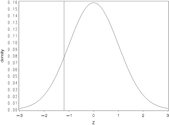
Denote the underlying, unobservable random variable by Z and suppose that Z is associated with a predictor variable X according to the linear regression equation, Z = β0 + β1X. Remember, you cannot observe Z; all you can observe is the consequences of Z. If Z is below a certain level, you observe a success. Otherwise, you observe a failure. The regression of Z on X models how the failure-success boundary changes with X. Figure 10.1 depicts a case for which the boundary, denoted ZX, for a given X is equal to –1.2. Thus, the area under the normal curve below ZX=–1.2 is the probability of a success for the corresponding X. As X changes, the boundary value ZX changes, thereby altering the probability of a success.
Formally, the standard normal cumulative distribution function, that is, the area under the curve less than Z, is denoted Φ(z) Thus, the probit linear regression model can be written π = Φ(β0 + β1X). Note that this give the model in the form of the inverse link. You can write the probit model in terms of the link function as probit(π) Φ−1(π) = β0 + β1X, where Φ−1 where (π) means the Z value such that the area under the curve less than Z is π.
You can fit the probit regression model to the O-ring data using the following SAS statements:
proc genmod data=agr_135;
model td/total=temp/ link=probit type1;
Note the use of the LINK=PROBIT option but no DIST option. Because of the ratio response variable, the binomial distribution is assumed by default, but a LINK statement is required because the PROBIT link is not the default. The results appear in Output 10.7.
Output 10.7 GENMOD Results Fitting the PROBIT Link to O-Ring Data
Criteria For Assessing Goodness Of Fit
| Criterion | DF | Value | Value/DF |
| Deviance | 14 | 12.0600 | 0.8614 |
| Scaled Deviance | 14 | 12.0600 | 0.8614 |
| Pearson Chi-Square | 14 | 10.9763 | 0.7840 |
| Scaled Pearson X2 | 14 | 10.9763 | 0.7840 |
Analysis Of Parameter Estimates
| Parameter | DF | Estimate | Standard Error |
Wald 95% Confidence Limits |
Chi- Square |
Pr > ChiSq | |
| Intercept | 1 | 8.7750 | 4.0286 | 0.8790 | 16.6709 | 4.74 | 0.0294 |
| temp | 1 | -0.1351 | 0.0584 | -0.2495 | -0.0206 | 5.35 | 0.0207 |
LR Statistics For Type 1 Analysis
| Source | Deviance | DF | Chi- Square |
Pr > ChiSq |
| Intercept | 19.9494 | |||
| temp | 12.0600 | 1 | 7.89 | 0.0050 |
The results are not strikingly different from the results of the logistic regression. The deviance is 12.060 (versus 11.997 for the logit link) and the p-value for the likelihood ratio test of H0: β1=0 is 0.0050 (versus 0.0320 using the logit link). The estimate of β1 is different, reflecting a different scale for the probit versus the logit. However, the sign and conclusion regarding the effect of temperature on thermal distress is the same.
You can use the ESTIMATE statements as shown in Output 8.3 to obtain predicted probits for various temperatures. You use the inverse link, π(estimate), to convert predicted probits to predicted probabilities. The SAS function to evaluate Φ(estimate) is PROBNORM. You use the following SAS statements to obtain the probit model analog to Output 10.4:
estimate 'probit at 50 deg' intercept 1 temp 50;
estimate 'probit at 60 deg' intercept 1 temp 60;
estimate 'probit at 64.7 deg' intercept 1 temp 64.7;
estimate 'probit at 64.8 deg' intercept 1 temp 64.8;
estimate 'probit at 70 deg' intercept 1 temp 70;
estimate 'probit at 80 deg' intercept 1 temp 80;
ods output estimates=probit;
run;
data prob_hat;
set probit;
phat=probnorm(estimate);
pi=3.14159;
invsqrt=1/(sqrt(2*pi));
se_phat=invsqrt*exp(-0.5*(estimate**2))*stderr;
prb_LcL=probnorm(LowerCL);
prb_UcL=probnorm(UpperCL);
proc print data=prob_hat;
The results appear in Output 10.8. Note the form of the Delta Rule for the probit model to obtain the approximate standard error of . This follows from the fact that the approximate standard error of using the Delta Rule, is s.e.(η). The derivative = = .
Output 10.8 Predicted Probits and Probabilities Obtained from the PROBNORM Inverse Link and the Probit Form of the Delta Rule
| Obs | Label | Estimate | StdErr | Alpha | LowerCL | UpperCL |
| 1 | probit at 50 deg | 2.0201 | 1.1413 | 0.05 | -0.2167 | 4.2570 |
| 2 | probit at 60 deg | 0.6692 | 0.6024 | 0.05 | -0.5115 | 1.8498 |
| 3 | probit at 64.7 deg | 0.0342 | 0.3960 | 0.05 | -0.7420 | 0.8104 |
| 4 | probit at 64.8 deg | 0.0207 | 0.3925 | 0.05 | -0.7487 | 0.7901 |
| 5 | probit at 70 deg | -0.6818 | 0.3244 | 0.05 | -1.3175 | -0.0461 |
| 6 | probit at 80 deg | -2.0328 | 0.7277 | 0.05 | -3.4590 | -0.6066 |
| Obs | ChiSq | Prob ChiSq |
phat | pi | invsqrt | se_phat | prb_LcL | prb_UcL |
| 1 | 3.13 | 0.0767 | 0.97832 | 3.14159 | 0.39894 | 0.05917 | 0.41421 | 0.99999 |
| 2 | 1.23 | 0.2666 | 0.74831 | 3.14159 | 0.39894 | 0.19211 | 0.30450 | 0.96783 |
| 3 | 0.01 | 0.9312 | 0.51365 | 3.14159 | 0.39894 | 0.15790 | 0.22905 | 0.79115 |
| 4 | 0.00 | 0.9579 | 0.50826 | 3.14159 | 0.39894 | 0.15657 | 0.22703 | 0.78526 |
| 5 | 4.42 | 0.0356 | 0.24768 | 3.14159 | 0.39894 | 0.10257 | 0.09383 | 0.48163 |
| 6 | 7.80 | 0.0052 | 0.02104 | 3.14159 | 0.39894 | 0.03678 | 0.00027 | 0.27207 |
Comparing Output 10.8 to the analogous output for the logistic model in Output 10.4, the estimated probabilities, approximate standard errors, and lower and upper confidence limits are similar, though not equal, for the two models. For example, for the logit model, at 50˚ , the predicted probability of thermal distress was 0.969 with an approximate standard error of 0.061, whereas for the probit model the predicted probability (PHAT) is 0.978, with an approximate standard error of 0.059. Other “discrepancies” are similarly small; you reach essentially the same conclusions about the O-ring data with either link function.
In general, the logit and probit models produce similar results. In fact, the logit and probit are very similar functions of π, so the fact that they produce similar results is not surprising. There are no compelling statistical reasons to choose one over the other. In some studies, you use the logistic model because its interpretation in terms of odds-ratios fits the subject matter. In other disciplines, the probit model of the mean has a theoretical basis, so the probit is preferred.
10.3 Binomial Models for Analysis of Variance and Analysis of Covariance
Logit and probit link functions are not limited to regression models. You can use them in conjunction with any of the classification models—one-way, two-way, and so forth—used in analysis of variance with normally distributed data. This allows you to perform the equivalent of analysis of variance for non-normal data. You can also fit the logit and probit links to analysis-of-covariance models. This section presents two examples, one for analysis of variance, the other for analysis of covariance. The analysis of variance example uses both the logit link (Section 10.3.1) and the probit link (Section 10.3.2). Section 10.3.3 presents analysis of covariance with a logit link.
10.3.1 Logistic ANOVA
Output 10.9 shows data from a clinical trial comparing two treatments, an experimental drug versus a control.
Output 10.9 Binomial Clinical Trial Data
| Obs | clinic | trt | fav | unfav | nij |
| 1 | 1 | drug | 11 | 25 | 36 |
| 2 | 1 | cntl | 10 | 27 | 37 |
| 3 | 2 | drug | 16 | 4 | 20 |
| 4 | 2 | cntl | 22 | 10 | 32 |
| 5 | 3 | drug | 14 | 5 | 19 |
| 6 | 3 | cntl | 7 | 12 | 19 |
| 7 | 4 | drug | 2 | 14 | 16 |
| 8 | 4 | cntl | 1 | 16 | 17 |
| 9 | 5 | drug | 6 | 11 | 17 |
| 10 | 5 | cntl | 0 | 12 | 12 |
| 11 | 6 | drug | 1 | 10 | 11 |
| 12 | 6 | cntl | 0 | 10 | 10 |
| 13 | 7 | drug | 1 | 4 | 5 |
| 14 | 7 | cntl | 1 | 8 | 9 |
| 15 | 8 | drug | 4 | 2 | 6 |
| 16 | 8 | cntl | 6 | 1 | 7 |
The study was conducted at eight clinics. At each clinic, patients were assigned at random to either the experimental drug or the control. Denote nij as the number of patients (NIJ in the SAS data set) at the jth clinic assigned to the ith treatment. At the end of the trial, patients either had favorable or unfavorable responses to treatment. For each treatment-clinic combination, the number of patients with favorable (FAV) and unfavorable (UNFAV) responses was recorded.
Beitler and Landis (1985) discussed these data assuming that CLINIC constituted a random effect. Littell et al. (1996) used the data as an example of a generalized linear mixed model, again assuming random clinic effects. This section presents a simpler analysis, using PROC GENMOD, assuming that the design can be viewed as a randomized-blocks design with CLINIC assumed to be a fixed-blocks effect.
Assuming the RCBD with fixed blocks, a model for the data is
logit(πij) = β + τi + βj,
where
| πij | is the probability of a favorable response for the ith treatment at the jth clinic (i = 1, 2; j = 1, 2,...,8). |
| β | is the intercept. |
| τi | is the effect of the ith treatment. |
| βj | is the effect of the jth clinic. |
Note that the response variable is FAV, the number of patients having favorable responses, or, alternatively, the sample proportion, FAV/NIJ. However, generalized linear models are given in terms of the link function, rather than the response variable, on the left-hand side of the model equation.
You can run the analysis using the SAS statements
proc genmod;
class clinic trt;
model fav/nij=clinic trt/dist=binomial link=logit type3;
run;
Output 10.10 shows the results of interest for this analysis.
Output 10.10 Logistic ANOVA for Binomial Clinical Trial Data
The GENMOD Procedure
Model Information
| Data Set | WORK.A |
| Distribution | Binomial |
| Link Function | Logit |
| Response Variable (Events) | fav |
| Response Variable (Trials) | nij |
| Observations Used | 16 |
| Number Of Events | 102 |
| Number Of Trials | 273 |
Class Level Information
| Class | Levels | Values |
| clinic | 8 | 1 2 3 4 5 6 7 8 |
| trt | 2 | cntl drug |
Criteria For Assessing Goodness Of Fit
| Criterion | DF | Value | Value/DF |
| Deviance | 7 | 9.7463 | 1.3923 |
| Scaled Deviance | 7 | 9.7463 | 1.3923 |
| Pearson Chi-Square | 7 | 8.0256 | 1.1465 |
| Scaled Pearson X2 | 7 | 8.0256 | 1.1465 |
| Log Likelihood | -138.5100 | ||
Algorithm converged.
LR Statistics For Type 3 Analysis
| Source | DF | Chi- Square |
Pr < ChiSq |
| clinic | 7 | 81.21 | <.0001 |
| trt | 1 | 6.67 | 0.0098 |
The first part of the output gives the model and class level information. You use this to verify that GENMOD is interpreting the data and your model instructions correctly.
The important items in the output are the “Criteria for Assessing Goodness of Fit” and the “LR Statistics for Type 3 Analysis.” You use the goodness-of-fit criteria as they were used for logistic regression. At α=0.25, the table =9.04 and at α=0.10, =12.02. Neither the deviance, 9.7463, nor the Pearson π2, 8.0256, gives evidence of significant lack of fit. The Type 3 likelihood ratio statistics are equivalent to the analysis of variance results for hypotheses based on Type 3 estimable functions for data with normally distributed errors. The LR π2 statistic for CLINIC is 81.21 with 7 degrees of freedom. As in the case of conventional ANOVA, formal testing of hypotheses about blocking criteria is questionable, but you can interpret the large π2 value as evidence of clinic differences and hence the effectiveness of blocking by CLINIC. The main conclusion follows from the LR test for treatment. Based on the π2 of 6.67 and its p-value of 0.0098, you reject H0: τ1=τ2 and thus conclude that there is a statistically significant treatment effect.
You can compute LS means just as you can with conventional ANOVA. After the model statement in the GENMOD statements above, add the command:
lsmeans trt;
This produces the results given in Output 10.11. The estimate and standard error are given on the logit scale. For example, for CNTL, the control treatment, the LS mean is –1.2554 with a standard error of 0.2692. This is the estimated logit that results from computing The chi-square values are the Wald statistics to test H0: LSMEAN (TRT i) = 0. On the logit scale, LSMEAN=0 implies that the log odds for the ith treatment is 0 or the odds equal 1.
Output 10.11 Least-Squares Means for Binomial Clinical Trial Data
Least Squares Means
| Effect | trt | Estimate | Standard Error |
DF | Chi- Square |
Pr > ChiSq |
| trt | cntl | -1.2554 | 0.2692 | 1 | 21.74 | <.0001 |
| trt | drug | -0.4784 | 0.2592 | 1 | 3.41 | 0.065 |
If you want the equivalent of the least-squares mean for the probability of a favorable outcome, you need to use the inverse link. Section 8.3.1 showed you how to use the inverse link to get the probability, the Delta Rule for the standard error, and how to obtain upper and lower confidence limits. For the control treatment, the estimated probability is and the standard error of , the “LS Mean of treatment 1,” is approximately 0.22*(1–0.22)*(0.2692)=0.046. As shown in Section 8.3.1, you can use ODS statements to output the logit-scale LS means and apply the inverse link and Delta Rule to convert them to the probability scale. You add the following statement to GENMOD after the LSMEANS statement:
ods output lsmeans=lsm;
and then run the following:
data prob_hat;
set lsm;
phat=exp(estimate)/(1+exp(estimate));
se_phat=phat*(1-phat)*stderr;
proc print data=prob_hat;
run;
Output 10.12 shows the results. PHAT is the LS mean probability for the ith treatment.
Output 10.12 LS Means Converted to Probability Scale for Binomial Clinical Trial Data
| Obs | Effect | trt | Estimate | StdErr | DF | ChiSq | ChiSq | phat | se_phat |
| 1 | trt | cntl | -1.2554 | 0.2692 | 1 | 21.74 | <.0001 | 0.22177 | 0.046467 |
| 2 | trt | drug | -0.4784 | 0.2592 | 1 | 3.41 | 0.0650 | 0.38262 | 0.061238 |
GENMOD allows you to use the ESTIMATE and CONTRAST statements. You include these statements after the MODEL statement. They can go either before or after the LSMEANS statement, if you are using both. Here are typical examples:
estimate 'lsm - cntl' intercept 1 trt 1 0;
estimate 'lsm - drug' intercept 1 trt 0 1;
estimate 'diff' trt 1 -1;
contrast 'diff' trt 1 -1;
You can see that the syntax is identical to other SAS PROCs, such as GLM and MIXED. Output 10.13 shows the results.
Output 10.13 ESTIMATE and CONTRAST Results for Binomial Clinical Trial Data
Contrast Estimate Results
| Label | Estimate | Standard Error |
Alpha | Confidence Limits | Chi- Square |
Pr > ChiSq | ||
| lsm - cntl | -1.2554 | 0.2692 | 0.05 | -1.7830 | -0.7277 | 21.74 | <.0001 | |
| lsm - drug | -0.4784 | 0.2592 | 0.05 | -0.9865 | 0.0297 | 3.41 | 0.0650 | |
| diff | -0.7769 | 0.3067 | 0.05 | -1.3780 | -0.1758 | 6.42 | 0.0113 | |
Contrast Results
| Contrast | DF | Chi- Square |
Pr > ChiSq | Type |
| diff | 1 | 6.67 | 0.0098 | LR |
The estimates LSM-CNTL and LSM-DRUG are the treatment least-squares means; the statistics are identical to those discussed earlier for the LS means. The estimate of DIFF is and the associated chi-square is the Wald statistic for testing H0: τ1 − τ2 =0. The CONTRAST statement computes a test for H0: τ1 − τ2, but it uses the likelihood ratio statistic. You can see that the two statistics are similar and would thus result in similar conclusions. As mentioned in Section 8.3, there is no clear evidence in favor of the Wald or likelihood ratio statistic relative to the other.
Caution: You cannot convert a difference to the probability scale using the inverse link—it results in nonsense. For example, on the logit scale, =–0.7769, thus the inverse link is = 0.32. However, from the previous discussion of the LS means, the difference between and was approximately 0.16. Because the logit is a non-linear function, differences are not preserved when the function or its inverse is applied.
You can interpret as the log of the odds-ratio between the treatments. An odds-ratio of 1, and hence a log odds-ratio of 0 mean that the odds, for example, of favorable versus unfavorable response, are the same for the two treatments. A significant negative log odds means that the odds of a favorable response are lower for the control than they are for the experimental drug, evidence that the experimental drug is effective. You can also see this reflected in the estimates of and given earlier.
An alternative model for these data includes a term for the treatment-clinic interaction. The model is
logit(πij) = μ + τi + βj+ (τβ)ij,
where (τβ)ij is the treatment-clinic interaction for the ith treatment and jth clinic and all other terms are as previously defined. The SAS statements for the model are
proc genmod data=a;
class clinic trt;
model fav/nij=clinic trt clinic*trt/dist=binomial
link=logit type3;
These statements are identical to the SAS program for the model without (τβ)ij except for the addition of the CLINIC*TRT term to the model. Output 10.14 gives the goodness-of-fit statistics and the ANOVA analog, that is, the Type 3 likelihood ratio statistics.
Output 10.14 Goodness of Fit and Likelihood Ratio Type 3 ANOVA of a Model with an Interaction for Binomial Clinical Trial Data
Criteria For Assessing Goodness Of Fit
| Criterion | DF | Value | Value/DF |
| Deviance | 0 | 0.0000 | . |
| Pearson Chi-Square | 0 | 0.0000 | . |
LR Statistics For Type 3 Analysis
| Source | DF | Chi- Square |
Pr > ChiSq |
| clinic | 7 | 83.14 | <.0001 |
| trt | 1 | 5.86 | 0.0155 |
| clinic*trt | 7 | 9.75 | 0.2034 |
For the model with interaction, there are 0 degrees of freedom for the goodness-of-fit statistics. This is a saturated model because there are 16 treatment clinic combinations, and hence 15 total degrees of freedom, all of which are used in the model. Also, the CLINIC*TRT likelihood ratio π2 statistic has the same degrees of freedom and the same value, 9.75, as the deviance in the no-interaction model. In fact, the likelihood ratio π2 for CLINIC*TRT and the deviance in the no-interaction model are the same statistic, expressed in different ways. In general, the deviance in ANOVA-type generalized linear models is the sum of all effects—typically interaction effects—left out of the model. In principle, this is similar to using interaction effects assumed to be zero in place of MS(ERROR) in standard ANOVA models.
10.3.2 The Analysis-of-Variance Model with a Probit Link
Just as you saw with regression in Section 10.2, you can fit an analysis-of-variance model to binomial data using a logit or probit link. In many cases, a mathematical model that follows from underlying theory in a given discipline provides the link function. Probit analysis, data analysis using a generalized linear model for binomial data with a probit link, is a common example of a subject matter theory-driven approach. For example, quantitative genetics has a well-developed theory framed in terms of the normal distribution. The probit link allows this theory to be adapted easily to Bernoulli response variables.
The basic premise of the probit link is that there exists an unobservable, normally distributed process. The observable consequence of the process is a Bernoulli random variable. For example, in the Beitler and Landis (1985) binomial clinic trial data, imagine that there is a continuous random variable roughly defined as the amount of disease stress to which the patient is subjected. The actual disease stress random variable cannot be measured. If the disease stress is sufficient, we observe an unfavorable outcome. Otherwise, we observe a favorable outcome. Only the favorable or unfavorable Bernoulli response variable is observable.
A probit model for the data shown in Output 10.9 is
probit(πij) = Φ–1(ij) = μ + τi + βj
where μ, τi, and βj are the intercept, treatment effect, and block effect as defined in Section 8.4.1. You use the following statements for the analysis:
proc genmod data=a;
class clinic trt;
model fav/nij=clinic trt/dist=binomial link=probit type3;
lsmeans trt;
estimate 'lsm - cntl' intercept 1 trt 1 0;
estimate 'lsm - drug' intercept 1 trt 0 1;
estimate 'diff' trt 1 -1;
contrast 'diff' trt 1 -1;
The only difference between the GENMOD statement above and the logistic ANOVA in Section 10.3.1 is the substitution of LINK=PROBIT in the above MODEL statement in place of LINK=LOGIT. Note that if you leave out the LINK= statement, GENMOD uses the logit link by default, because it is the canonical link for the binomial distribution. If you want to use the probit link, you must use the LINK=PROBIT option. Output 10.15 shows the results.
Output 10.15 Analysis of Binomial Clinical Trial Data Using the Probit Link
Criteria For Assessing Goodness Of Fit
| Criterion | DF | Value | Value/DF |
| Deviance | 7 | 9.6331 | 1.3762 |
| Pearson Chi-Square | 7 | 8.0048 | 1.1435 |
Analysis Of Parameter Estimates
| Parameter | DF | Estimate | Standard Error |
Wald 95% Confidence Limits |
Chi- Square |
||
| Intercept | 1 | 0.9792 | 0.3934 | 0.2082 | 1.7503 | 6.20 | |
| clinic 1 | 1 | -1.3158 | 0.4120 | -2.1233 | -0.5082 | 10.20 | |
| clinic 2 | 1 | -0.0678 | 0.4254 | -0.9014 | 0.7659 | 0.03 | |
| clinic 3 | 1 | -0.6120 | 0.4339 | -1.4625 | 0.2385 | 1.99 | |
| clinic 4 | 1 | -2.1118 | 0.4922 | -3.0765 | -1.1472 | 18.41 | |
| clinic 5 | 1 | -1.6482 | 0.4695 | -2.5685 | -0.7280 | 12.32 | |
| clinic 6 | 1 | -2.4909 | 0.6171 | -3.7004 | -1.2813 | 16.29 | |
| clinic 7 | 1 | -1.7758 | 0.5666 | -2.8862 | -0.6653 | 9.82 | |
| clinic 8 | 0 | 0.0000 | 0.0000 | 0.0000 | 0.0000 | . | |
| trt cntl | 1 | -0.4587 | 0.1778 | -0.8072 | -0.1101 | 6.65 | |
| trt drug | 0 | 0.0000 | 0.0000 | 0.0000 | 0.0000 | . | |
LR Statistics For Type 3 Analysis
| Source | DF | Chi- Square |
Pr > ChiSq |
| clinic | 7 | 81.33 | <.0001 |
| trt | 1 | 6.78 | 0.0092 |
Least Squares Means
| Effect | trt | Estimate | Standard Error |
DF | Chi- Square |
Pr > ChiSq |
| trt | cntl | -0.7322 | 0.1481 | 1 | 24.45 | <.0001 |
| trt | drug | -0.2735 | 0.1407 | 1 | 3.78 | 0.0518 |
Contrast Estimate Results
| Label | Estimate | Standard Error |
Alpha | Confidence Limits | Chi- Square |
Pr > ChiSq | |
| lsm - cntl | -0.7322 | 0.1481 | 0.05 | -1.0224 | -0.4420 | 24.45 | <.0001 |
| lsm * drug | -0.2735 | 0.1407 | 0.05 | -0.5493 | 0.0022 | 3.78 | 0.0518 |
| diff | -0.4587 | 0.1778 | 0.05 | -0.8072 | -0.1101 | 6.65 | 0.0099 |
Contrast Results
| Source | DF | Chi- Square |
Pr > ChiSq | Type |
| diff | 1 | 6.78 | 0.0092 | LR |
There are minor differences between the results, but the overall conclusions are similar. The deviance for the logit model was 9.7463; here it is 9.6331. The likelihood ratio π2 for the test of no treatment effect, H0: τ1=τ2, was 6.67 for the logit model; here it is 6.78. The major difference is in the estimates of the intercept μ, the treatment effects τi, the clinic effects βj, and the results estimates and least-squares means. These are estimated on the probit scale, and hence the estimates and standard errors are different.
As with the logistic model, in most practical situations, you will want to use the inverse link to convert estimates from the probit scale to the probability scale, and use the Delta Rule to convert the standard error. As with the logistic model, you can use the ODS statement to output LSMEANS or ESTIMATES and then use program statements to compute the inverse link and Delta Rule. For the LSMEANS, you follow these steps:
1. Insert ods output lsmeans=lsm; into the GENMOD program.
2. Run these program statements:
data prob_hat;
set lsm;
phat=probnorm(estimate);
pi=3.14159;
invsqrt=1/(sqrt(2*pi));
se_phat=invsqrt*exp(-0.5*(estimate**2))*stderr;
proc print data=prob_hat;
run;
You can also add upper and lower confidence limits, as shown in Section 10.3.1. The statements are identical except you use the PROBNORM inverse link. Output 10.16 shows the result for and its standard error.
Output 10.16 Probability of Favorable Outcome—Estimate and Standard Error from a Probit Link Model
| Obs | Effect | trt | Estimate | StdErr | DF | ChiSq |
| 1 | trt | cntl | -0.7322 | 0.1481 | 1 | 24.45 |
| 2 | trt | drug | -0.2735 | 0.1407 | 1 | 3.78 |
| Obs | Prob ChiSq |
phat | pi | invsqrt | se_phat |
| 1 | <.0001 | 0.23202 | 3.14159 | 0.39894 | 0.045181 |
| 2 | 0.0518 | 0.39222 | 3.14159 | 0.39894 | 0.054060 |
You can see that the estimated probabilities (PHAT), 0.23 and 0.39 for control and drug treatments, respectively, are slightly different from the 0.22 and 0.38 obtained using the logit link. Also, the standard errors (SE_PHAT) are somewhat different from those obtained from the logit model. However, the differences are slight, and the overall conclusions you would reach from these two models are very similar.
The same comments made at the end of Section 10.2 about logistic versus probit regression also apply to logit versus probit analysis-of-variance models. They typically produce similar results. The main reason to choose one link over the other often has to do with the subject matter of the study. Some disciplines characterize binomial data mainly by using odds ratios; because logistic models have natural interpretations in terms of odds ratios, they are an obvious choice. Other areas, such as quantitative genetics, have a well-developed theory expressed in terms of the normal distribution. For these disciplines, the probit model has obvious advantages.
10.3.3 Logistic Analysis of Covariance
Output 10.17 shows data from a bioassay involving two drugs, standard (STD) and treated (TRT) injected in varying dosages to 20 mice per treatment-dose combination. The response variable of interest is the number of mice out of the 20 that are ALIVE versus the number DEAD. These data appear in Koch et al. (1975) and are discussed in Freeman’s (1987) text.
Output 10.17 Treatment-Dose Bioassay Data
| Obs | drug | dosage | alive | dead | total |
| 1 | std | 1 | 19 | 1 | 20 |
| 2 | std | 2 | 15 | 5 | 20 |
| 3 | std | 4 | 11 | 9 | 20 |
| 4 | std | 8 | 4 | 16 | 20 |
| 5 | std | 16 | 1 | 19 | 20 |
| 6 | trt | 1 | 16 | 4 | 20 |
| 7 | trt | 2 | 12 | 8 | 20 |
| 8 | trt | 4 | 5 | 15 | 20 |
| 9 | trt | 8 | 2 | 18 | 20 |
As discussed in Freeman’s text, the researchers wanted to know how DRUG and DOSAGE affected the probability of a dead mouse. Their objectives suggested analysis of covariance to answer the following specific questions:
❏ Was there a dosage effect?
❏ Was the dosage effect the same for the two DRUG groups?
❏ Was there a significant difference between the DRUG groups, adjusted for constant dosage?
You can use PROC GENMOD to compute logistic analysis of covariance to answer these questions. Following Freeman, this example uses X=log2(DOSAGE) as the covariate. A generalized linear model for these data is
logit(πij)=μ+τi + (β+δi)X
where
| πij | is the probability of a dead mouse given the ith treatment (DRUG group) and the jth dosage. |
| μ | is the intercept. |
| τi | is the effect of the ith treatment. |
| β | is the slope for the regression of X on the logit. |
| δi | is the effect of the ith treatment on the slope. |
Alternatively, you can give the above model as
logit(πij)= β0i + β1i X
where
| β0i = μ+τi | is the intercept for the ith treatment. |
| β1i = β + δi | is the slope for the ith treatment. |
The first form of the model allows you an easy test for equal slopes, that is, H0: all δi=0. The second form of the model allows easier characterization of the regression equation for each DRUG group.
You can compute the analysis for the μ+τi + (β+δi) X form of the model using these statements:
proc genmod;
class drug;
model dead/total=drug x drug*x
/dist=bin link=logit type1;
run;
In the model, DRUG corresponds to τi, X corresponds to β, and X*DRUG corresponds to δi. Output 10.18 gives the relevant results.
Output 10.18 Logistic Analysis of Covariance to Test for Unequal Slopes
Criteria For Assessing Goodness Of Fit
| Criterion | DF | Value | Value/DF |
| Deviance | 5 | 0.7464 | 0.1493 |
| Scaled Deviance | 5 | 0.7464 | 0.1493 |
| Pearson Chi-Square | 5 | 0.7541 | 0.1508 |
| Scaled Pearson X2 | 5 | 0.7541 | 0.1508 |
LR Statistics For Type 1 Analysis
| Source | Deviance | DF | Chi- Square |
Pr < ChiSq |
| Intercept | 80.6276 | |||
| drug | 79.9301 | 1 | 0.70 | 0.4036 |
| x | 0.8580 | 1 | 79.07 | <.0001 |
| x*drug | 0.7464 | 1 | 0.11 | 0.7383 |
You can see from the goodness-of-fit statistics that there is no evidence of lack of fit. The likelihood ratio π2 for X*DRUG tests H0:δi=0, the hypothesis of equal slopes for the drug groups.
You can also test the hypothesis of equal slopes and at the same time estimate the regressions for each DRUG group using the β0i + β1iX form of the model. Here are the required SAS statements:
proc genmod;
class drug;
model alive/total=drug x(drug)/dist=bin link=logit noint;
contrast 'equal slope?' x(drug) 1 -1;
As in other SAS linear model programs, the NOINT option in the MODEL statement suppresses the intercept, so that DRUG in the model corresponds to β0i and X(DRUG) corresponds to β1i. Thus the CONTRAST statement computes the test statistic for H0: = β1i = β12 that is, the hypothesis of equal slopes for the two DRUG groups. Output 10.19 shows the relevant results.
Output 10.19 Logistic Analysis of Covariance: Estimates of Regression Equations for Each Group
Analysis Of Parameter Estimates
| Parameter | DF | Estimate | Standard Error |
Wald 95% Confidence Limits |
Chi- Square |
|
| drug std | 1 | 2.7345 | 0.5732 | 1.6111 | 3.8579 | 22.76 |
| drug trt | 1 | 1.4960 | 0.4633 | 0.5880 | 2.4040 | 10.43 |
| x(drug) std | 1 | -1.3673 | 0.2529 | -1.8630 | -0.8715 | 29.22 |
| x(drug) trt | 1 | -1.2404 | 0.2827 | -1.7945 | -0.6863 | 19.25 |
Analysis Of Parameter
Estimates
| Parameter | Pr > ChiSq |
| drug std | <.0001 |
| drug trt | 0.0012 |
| x(drug) std | <.0001 |
| x(drug) trt | <.0001 |
Contrast Results
| Contrast | DF | Chi- Square |
Pr > ChiSq | Type |
| equal slope? | 1 | 0.11 | 0.7383 | LR |
You can see that the likelihood ratio χ2 in the “Contrast Results” for the test of equal slopes is identical to the previous result for X*DRUG. The two are alternative ways to compute the same statistic. The deviance and Pearson χ2 goodness-of-fit statistics are also the same (not shown for the latter model). From the output, you can see that the estimated regression equation for the DRUG STD is 2.7345–1.3673*X, and for the DRUG TRT it is 1.4960–1.2404*X. You could determine these regression coefficients from the program using the former model that produced Output 10.18 by using appropriately defined ESTIMATE statements.
Because there is no evidence of unequal slopes, the next step is to fit the equal slopes analysis-of-covariance model
logit(πij)=μ+τi + βX
where the terms in the model are defined as given above. Use the following program to compute the analysis:
proc genmod;
class drug;
model alive/total=drug x /dist=bin link=logit type1 type3;
Output 10.20 shows the results.
Output 10.20 Equal Slopes Analysis of Covariance for Treatment-Dose Bioassay Data
Analysis Of Parameter Estimates
| Parameter | DF | Estimate | Standard Error |
Wald 95% Confidence Limits |
Chi- Square |
|
| Intercept | 1 | 1.5923 | 0.3707 | 0.8658 | 2.3187 | 18.45 |
| drug std | 1 | 1.0337 | 0.4031 | 0.2437 | 1.8237 | 6.58 |
| drug trt | 0 | 0.0000 | 0.0000 | 0.0000 | 0.0000 | . |
| x | 1 | -1.3130 | 0.1875 | -1.6805 | -0.9455 | 49.02 |
LR Statistics For Type 1 Analysis
| Source | Deviance | DF | Chi- Square |
Pr < ChiSq |
| Intercept | 80.6276 | |||
| drug | 79.9301 | 1 | 0.70 | 0.4036 |
| x | 0.8580 | 1 | 79.07 | <.0001 |
LR Statistics For Type 3 Analysis
| Source | DF | Chi- Square |
Pr > ChiSq |
| drug | 1 | 7.04 | 0.0080 |
| x | 1 | 79.07 | <.0001 |
From the “Analysis of Parameter Estimates” you can see that the estimated regression coefficient is =1.313, with a standard error of 0.1875. The regression equation for the ith treatment is μ + τi + βX. For example, for the DRUG STD, the estimated regression equation is 1.5923+1.0337–1.313*X, or 2.626–1.313*X. For the DRUG TRT, the regression equation is 1.5923–1.313*X.
As with standard analysis of covariance, as presented in Chapter 7, the Type 1 analysis compares the DRUG STD with TRT at their respective mean X levels, rather than at a common value. The DRUG STD had a DOSAGE level of 16 (X=4) whereas TRT did not. Hence the mean of X for STD is 2, whereas the mean of X for TRT is only 1.5. Formally, the Type 1 likelihood ratio π2 tests H0:τSTD–τTRT+β(), that is, H0:τSTD–τTRT+β*0.5. Because the slope β is positive, the observed performance of STD is shifted upward relative to TRT resulting in a π2 of 0.70 (p=0.4036), making it appear that there is no statistically significant DRUG effect.
The Type 3 analysis compares STD with TRT at a common value of X—that is, H0:τSTD–τTRT, resulting in a likelihood ratio π2 of 7.04 (p=0.008). The DRUG STD effect of 1.0337 in the “Analysis of Parameter Estimates” estimates the magnitude of the DRUG effect for a common X. The chi-square of 6.58 is the Wald π2 to test the DRUG effect.
You can estimate least-squares means by adding the statement
lsmeans drug/e;
to the GENMOD statements given above. The E option prints the coefficients of the LS means, allowing you to see the value of X used to compute them. Output 10.21 gives the result.
Output 10.21 Least-Squares Means for Common Slope Analysis of Treatment-Dose Bioassay Data
Coefficients for drug Least Squares Means
| Label | Row | Prm1 | Prm2 | Prm3 | Prm4 |
| drug | 1 | 1 | 1 | 0 | 1.7778 |
| drug | 2 | 1 | 0 | 1 | 1.7778 |
Least Squares Means
| Effect | drug | Estimate | Standard Error |
DF | Chi- Square |
Pr > ChiSq |
| drug | std | 0.2918 | 0.2686 | 1 | 1.18 | 0.2774 |
| drug | trt | -0.7419 | 0.2884 | 1 | 6.62 | 0.0101 |
You can see that the LS means are computed at the overall =1.778. The estimates and standard errors are computed on the logit scale. You can use ODS output and program statements for the inverse link and Delta Rule, as shown in previous examples, to express the estimates and standard errors on the probability scale.
If you want to estimate the performance of the DRUG for X different from the default overall used in the LSMEANS statement, you can use ESTIMATE statements. For example, for the DRUG STD at dosages of 1 and 16, that is, X=0 and X=4, you use the following statements. Output 10.22 shows the results.
estimate 'STD at dose=1' intercept 1 drug 1 0 x 0;
estimate 'STD at dose=16' intercept 1 drug 1 0 x 4;
Output 10.22 Estimates of DRUG STD at Different Dosages
Contrast Estimate Results
| Label | Estimate | Standard Error |
Alpha | Confidence Limits | Chi- Square |
|
| diff | 1.0337 | 0.4031 | 0.05 | 0.2437 | 1.8237 | 6.58 |
| STD at dose=1 | 2.6260 | 0.4594 | 0.05 | 1.7255 | 3.5265 | 32.67 |
| STD at dose=16 | -2.6260 | 0.4594 | 0.05 | -3.5265 | -1.7255 | 32.67 |
The estimate gives the logit for each dosage. As with the LS means, you can convert these to probabilities using the inverse link. Output 10.22 also gives the results for the statement
estimate ‘diff’ trt 1 –1;
You can see that the estimate, standard error, and π2 values for DIFF are identical to those of DRUG STD in the “Analysis of Parameter Estimates.”
An alternative common-intercepts model uses β1i instead of μ + τi. Use the following SAS statements to compute the model. Output 10.23 shows the results.
proc genmod;
class drug;
model alive/total=drug x /dist=bin link=logit noint;
contrast 'trt effect' drug 1 -1;
estimate 'STD at dose=1' drug 1 0 x 0;
estimate 'STD at dose=16' drug 1 0 x 4;
The only difference between these statements and those shown earlier involves the intercept. In the MODEL statement, these statements use the NOINT (no intercept) option. NOINT suppresses μ so that DRUG estimates β1i instead of τi. In the ESTIMATE statements, the options remove references to INTERCEPT. Thus, DRUG 1 0 multiplies instead of τi by a coefficient of 1. The CONTRAST statement obtains a likelihood ratio test of the difference between β11 and β12 which is equivalent to testing H0:τ1–τ2. You can use the ESTIMATE statement as shown in the previous analysis, if you prefer.
Output 10.23 Alternative Common Slopes Analysis of Covariance for Treatment-Dose Bioassay Data
Analysis Of Parameter Estimates
| Parameter | DF | Estimate | Standard Error |
Wald 95% Confidence Limits |
Chi- Square |
|
| drug std | 1 | 2.6260 | 0.4594 | 1.7255 | 3.5265 | 32.67 |
| drug trt | 1 | 1.5923 | 0.3707 | 0.8658 | 2.3187 | 18.45 |
| x | 1 | -1.3130 | 0.1875 | -1.6805 | -0.9455 | 49.02 |
Contrast Estimate Results
| Label | Estimate | Standard Error |
Alpha | Confidence Limits | Chi- Square |
|
| STD at dose=1 | 2.6260 | 0.4594 | 0.05 | 1.7255 | 3.5265 | 32.67 |
| STD at dose=16 | -2.6260 | 0.4594 | 0.05 | -3.5265 | -1.7255 | 32.67 |
Contrast Results
| Contrast | DF | Chi- Square |
Pr > ChiSq | Type |
| trt effect | 1 | 7.04 | 0.0080 | LR |
The main advantage of computing the analysis this way is that the estimates of the intercepts, β1i for each treatment are already computed, and do not need to be calculated from β and τi. Also, you have the standard errors of the in this output, whereas in the previous output there was no way to determine them. This output is more convenient when you need to report the regression equations for each DRUG. All other aspects of the analysis are identical to the results given in Outputs 10.20 through 10.22.