10.4 Count Data and Overdispersion

The examples in the previous sections of this chapter involved categorical data. Generalized linear models are useful for other types of non-normal data as well. Many studies, for example, use counts as the primary response variable. This section presents a typical example.

Historically, statistical theory has placed counting processes in a framework that implies a Poisson distribution. However, recent work, particularly in biological settings such as agriculture, ecology, and environmental science, suggests that the Poisson distribution is often inappropriate for counts. The Poisson assumes that the mean and variance are equal. In biological settings, the birds, insects, plants, and so forth being counted tend to be more aggregated—that is, clustered together—than you would expect under the Poisson model. Thus, the variance tends to be larger than the mean, in many cases much larger. Overdispersion is said to occur when the variance is larger than expected under a given model.

There are two approaches to overdispersion in GzLMs. First, you can use the GzLM assuming a Poisson distribution, but adjust standard errors and test statistics, as suggested by McCullagh and Nelder (1989). Alternatively, you can use a different distribution. For example, agricultural and ecological count data are often accurately characterized by the negative binomial distribution (Young and Young 1998).

This section uses an example of insect count to illustrate the main features of count models. Section 10.4.1 shows the standard Poisson model with no adjustments. Section 10.4.2 shows some basic model-checking procedures you can do with PROC GENMOD. Section 10.4.3 shows you how to do the overdispersion correction suggested by McCullagh and Nelder (1989). Section 10.4.4 presents an alternative model assuming the negative binomial and shows you how to fit it using PROC GENMOD.

10.4.1 An Insect Count Example

Output 10.24 contains data from an insect control experiment. The treatment design consisted of an untreated control and a 3×3 factorial for a total of ten treatments. The experiment was conducted as a randomized-complete-blocks design with four blocks. The response variable was insect count. TRT 0 is the control. The variable CTL_TRT is coded 0 for control and 1 otherwise. The two treatment factors, A and B, have three levels each (1, 2, and 3) and are both coded 0 for the control.

Output 10.24 Insect Count Data

As mentioned above, historically, the Poisson distribution has been assumed for count data. Using the Poisson canonical link, a GLM for these data is

log(λ_ij) = μ + γ_i + τ_j

where

λij	is the mean count for the ith block (i = 1, 2, 3, 4) and jth treatment (j = 0, 1,...,9).
μ	is the intercept.
γi	is the ith block effect.
τj	is the jth treatment effect.

The treatment effect can be expanded to account for control versus treated and the factorial treatment design. You partition it as

τ_jkl = δ_j + τ_k + β_?l + (τβ)_kl

where

δj	is the contrast between control and treated (j = 0, 1).
τk	is the main effect of the kth level of factor A (k = 1, 2, 3).
βl	is the main effect of the lth level of factor B (k = 1, 2, 3).
(τβ)kl	is the klth A×B interaction effect.

Use the following SAS statements to compute the analysis:

proc genmod data=a;
 class block ctl_trt a b;
 model count=block ctl_trt a b a*b/dist=poisson type1
type3;

The MODEL statement allows you to partition the treatment effects according to the model for τ_jkl given above. The LINK= option is omitted, but the DIST=POISSON statement causes the canonical link for the Poisson—the log link—to be fitted by default. Output 10.25 shows the results of the Type 1 and Type 3 likelihood ratio tests. These results are discussed below. The goodness-of-fit statistics are shown in Section 10.4.2.

Output 10.25 The First Version of the GENMOD Analysis of the Poisson Model for Insect Count Data

You could put only BLOCK and TRT in the CLASS and MODEL statements and use the CONTRAST statements to compute tests for the (CTL) versus (TRT), the main effects of A and B, and the A×B interaction. The SAS program is then

proc genmod data=a;
 class block trt;
 model count=block trt/dist=poisson type1 type3;
 contrast ‘ctl vs trt’ trt 9 -1 -1 -1 -1 -1 -1 -1 -1 -1;
 contrast ‘a’ trt 0 1 1 1 0 0 0 -1 -1 -1,
              trt 0 0 0 0 1 1 1 -1 -1 -1;
 contrast ‘b’ trt 0 1 0 -1 1 0 -1 1 0 -1,
              trt 0 0 1 -1 0 1 -1 0 1 -1;
 contrast ‘a x b’ trt 0 1 0 -1 0 0 0 -1 0 1,
                  trt 0 0 0 0 1 0 -1 -1 0 1,
                        trt 0 0 1 -1 0 0 0 0 -1 1,
                        trt 0 0 0 0 0 1 -1 0 -1 1;

Using A, B, and A*B in the MODEL statement as shown in the first program above is clearly more convenient than writing the equivalent contrasts. The results of the likelihood ratio tests for the contrasts in the second program appear in Output 10.26.

Output 10.26 Texts of Contrasts, the Second Version of the GENMOD Analysis of the Poisson Model for Insect Data

You can see that the TYPE3 likelihood ratio χ² statistics for A, B, and A*B in Output 10.25 are the same as you get when you use TRT in the model and write contrasts, shown in Output 10.26. The χ² statistic for A*B is 13.08 with a p-value of 0.0109, strong evidence of an A×B interaction.

The situation is not quite so simple for CTL_TRT. In Output 10.25, the Type I likelihood ratio χ² statistic is 39.90 with a p-value <0.0001. This statistic tests H₀:δ₀ =δ₁, using the partitioned form of the model for τ_jkl given above. The TYPE3 χ² statistic for CTL_TRT is 0 with 0 DF. This is because there are 0 levels of A and B, and the CTL_TRT effect is confounded with the 0 versus other levels of A and B comparisons. Hence, there are 0 degrees of freedom left for CTL_TRT once adjusted for A and B. Therefore, if you use the approach shown in Output 10.25, you must use the TYPE1 test for CTL_TRT, rather than the Type 3, and CTL_TRT must appear before A, B, and A*B in the MODEL statement. In Output 10.26, the control versus treated CONTRAST tests H₀:τ₀=$\frac{1}{9}{\displaystyle \sum _{j=1}^9{\tau }_j}$ . This results in a χ² statistic of 45.86, somewhat different from the test statistic obtained in Output 10.25. The discrepancy in the test statistics results from the non-linearity of the link function. The test statistics for CTL_TRT in the first SAS program and the control versus treated CONTRAST defined on TRT in the second form of the model would be identical under conventional, normal errors linear models—for example, using PROC GLM or PROC MIXED. In this example, the two approaches lead to identical conclusions about the difference between the control and the other treatments. We know of no definitive statistical reason to favor either approach over the other. This and related issues are the subject of ongoing research in generalized linear models. The first set of SAS statements is clearly more convenient, but you should check the CONTRAST as well to be sure the results are not in conflict.

10.4.2 Model Checking

Both GENMOD programs in Section 10.4.1 produce the goodness-of-fit statistics shown in Output 10.27.

Output 10.27 Goodness-of-Fit Statistics for Poisson GLM of Insect Count Data

Both the deviance and the Pearson χ² are greater than you would expect under the Poisson generalized linear model given in Section 10.4.1. This casts doubt on whether the Poisson model is appropriate and therefore whether the conclusions reached in the last section are valid.

There are a number of possible reasons for poor fit. Some of these reasons are familiar from conventional normal errors linear models. For example, the right-hand side of the model equation (κ + γ_i + τ_j) might be inadequate, in this case indicating a possible treatment×block interaction. Some of the reasons are unique to the generalized linear model, because of its added flexibility. The choice of probability distribution, or link function, or variance function, may be inappropriate. This section surveys model-checking procedures for GLMs you can do using PROC GENMOD. For more details, see generalized linear model texts such as McCullagh and Nelder (1989). Certain SAS procedures, for example, PROC LOGISTIC, have far more extensive model-checking facilities for certain specialized GLMs. These are not covered in this book.

McCullagh and Nelder suggest several plots to assist in identifying obvious problems with the model, including these:

• Plot standardized residuals against the predicted mean. This serves the same purpose as similar plots in conventional linear models. Unequal scatter indicates violation of the homogeneity of variance assumption. More generally, unequal scatter may suggest a poor choice of variance function. Systematic pattern may indicate a poor choice of Xβ, for example, fitting a linear regression to a quadratic pattern, or it may indicate a poor choice of link function or probability distribution.

• Plot y*, for example, $\widehat{\eta }+\frac{y-\widehat{\lambda }}{\widehat{\lambda }}$ for the Poisson, against, the estimated link function. This plot is unique to GLMs. The plot should be linear. Departure from linear suggests a poor choice of link function.

You can get these plots by using the GENMOD and PLOT procedures in SAS. For the insect count data and the Poisson model from Section 10.4.1, the SAS statements are

proc genmod data=a;
 class BLOCK trt;
 model count=BLOCK trt/dist=poisson type1 ObStats;
 ODS OUTPUT ObStats=check;
 title ‘compute model checking statistics’;

data plot;
 set check;
 adjlamda=2*sqrt(pred);
 ystar=xbeta+(count-pred)/pred;
 absres=abs(resdev);

options ps=28;
proc plot;
 plot resdev*(pred xbeta);
 plot (resdev reschi)*adjlamda;
 plot ystar*xbeta;
 plot absres*adjlamda;

The GENMOD statement is the same as you used to fit the Poisson model in Section 10.4.1, with the addition of an OBSTATS option to the MODEL statement and an ODS statement to output the OBSTATS to a new data set. The OBSTATS option computes several statistics analogous to predicted values and residuals for model checking in conventional linear models. The pertinent statistics are

STATISTIC	Definition
XBETA	estimate of link function, that is, $\widehat{\eta }=X\widehat{\beta }$
PRED	predicted value on COUNT scale, that is,${\widehat{\lambda }}_{ij}=h({\widehat{\eta }}_{ij})=\exp ({\widehat{\eta }}_{ij})$
RESDEV	residual deviance = sign(residual)*deviance of yij= $\text{sign(resid)}\times \text{[}\ell \text{(}{\lambda }_{ij};y_{ij})-\ell ({\lambda }_{ij};{\widehat{\lambda }}_{ij})]$
RESCHI	similar to residual deviance but uses component of Pearson χ2from ijth obs

The DATA PLOT step computes three additional functions of statistics in the OBSTATS output useful for model checking. McCullagh and Nelder (1989) suggest adjusting predicted values, in this case $\widehat{\lambda },$ to a constant information scale before plotting it against residual, because unadjusted predicted values may result in a misleading plot. For the Poisson, the adjustment is $2\sqrt{\widehat{\lambda }},$, ADJLAMDA in the SAS program. YSTAR is the linear predictor, y*=$\widehat{\eta }+\frac{\text{y}–\widehat{\lambda }}{\widehat{\lambda }},$ to be plotted against η̂ to check the link function. Finally, plotting the absolute value of the residuals as well as the residuals is often suggested, because the absolute values may reveal features the signed residuals miss. As an example, ABSRES is the absolute value of the residual deviance. You could also plot the absolute value of the residual χ². The plots generated by the PROC PLOT step are examples. Though not shown here, you could also do several plots using the residual χ² and plot absolute values of residuals against, say, XBETA as well as ADJLAMDA.

The example plots are shown below.

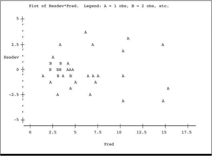
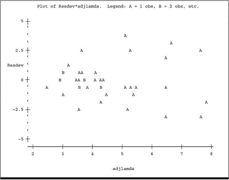
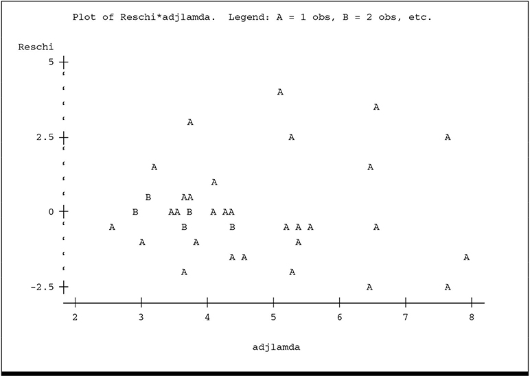
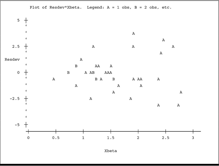
The plot of ADJLAMDA spreads the plot more evenly over the horizontal axis and reveals more detail for the lower predicted counts. While there is no overt visual evidence of unequal scatter or systematic pattern, there is a hint of lower variance among the residuals for the lowest predicted counts, especially on the ADJLAMDA plot. The plots of residual deviance against XBETA and residual π² against ADJLAMDA reveal similar information:

The plot of y* versus $\widehat{\mathrm{\eta }}$ is next. While there is scatter, there is no overt departure from linearity and hence no obvious evidence of a poor choice of link function.

Finally, the plot of absolute value of residual deviance versus ADJLAMDA reinforces the information contained in the previous residual plots.

There are two main results of this model-checking exercise:

1. The goodness-of-fit statistics, deviance, and Pearson χ² are larger than expected.

2. There is slight visual evidence that scatter among the residuals is not constant, but is lower for lower predicted counts.

Taken together, these symptoms indicate that the Poisson model may be inappropriate and, in particular, the assumed variance structure may not be correct. The next section discusses the likely reason as well as a commonly used adjustment.

10.4.3 Correction for Overdispersion

The Poisson model assumes that the mean and variance are equal. As mentioned previously, in biological counting processes the variance is typically greater than the mean. When the variance is larger than expected under a given model, the condition is called overdispersion. Unaccounted for overdispersion tends to cause standard errors to be underestimated and test statistics to be overestimated, resulting in excessive Type I error rates.

With generalized linear models, you have two ways to account for overdispersion—fit the Poisson model but adjust the standard errors and test statistics—or choose a different distribution for the model. This section shows you how to adjust the Poisson model. Section 10.4.4 gives an example of using PROC GENMOD to fit an alternative distribution.

You can model overdispersion by letting the actual variance equal the assumed variance multiplied by an additional scale parameter that adjusts for the discrepancy between assumed and actual. For the Poisson distribution, the assumed variance is the mean, ϕ, so the adjusted variance is ϕλ. Overdispersion occurs when ϕ>1. In GzLM literature, ϕ is typically referred to as the overdispersion parameter.

As a theoretical note, when you assume E(y)=λ and var(y)=ϕλ, you no longer have a true probability distribution for the random variable, y, but you do have a valid quasi-likelihood (see Section 10.6.4). You can show that for estimable Ḱβ from the resulting GLM, standard errors of $\text{K}\prime \widehat{\beta }$ are the standard errors you get from the Poisson model multiplied by $\sqrt{\varphi },$ and the Wald and likelihood ratio π² statistics are equal to the corresponding π² statistics divided by ϕ.

Because the overdispersion parameter is unknown, you must estimate it. McCullagh (1983) gives $\widehat{\varphi }$ = $\frac{(y-\widehat{\mu })\prime {\text{V}}_{\mu }^{-\text{1}}(y-\widehat{\mu })}{N-p}$ = $\frac{\text{Pearson }{\chi }^{\text{2}}}{N-p}$, where N–p is the degrees of freedom for lack of fit and V_μ is a diagonal matrix of variance functions defined in Section 10.6.2. McCullagh and Nelder (1989) also suggest using the deviance, that is, $\widehat{\varphi }=\frac{Deviance}{N-p}$.

You can compute the Poisson model corrected for overdispersion by using PROC GENMOD. For the insect count data, use the following SAS statements:

proc genmod data=a;
 class BLOCK CTL_TRT a b;
 model count=BLOCK CTL_TRT a b a*b/dist=poisson dscale
type1 type3;

This is the same set of statements used in Section 10.4.1 except for the addition of the DSCALE option in the MODEL statement. DSCALE causes all standard errors and test statistics to be corrected for a scale parameter estimated using the deviance, that is, $\widehat{\varphi }=\frac{Deviance}{N-p}.$ Alternatively, you can substitute PSCALE for DSCALE to get the scale parameter estimated by using the Pearson π². Output 10.28 shows the results:

Output 10.28 The Poisson Analysis of Insect Count Data Corrected for Overdispersion

The scaled deviance is the deviance divided by the estimated overdispersion parameter. Here, the overdispersion parameter is estimated by using the deviance, that is, $\widehat{\varphi }=\frac{93.9652}{27}$ =3.48. The scaled deviance is therefore equal to 1. In this context, the scaled goodness-of-fit statistics have no real interpretation except to indicate whether subsequent adjustment of standard errors and test statistics used a scale parameter estimate based on the deviance or the Pearson χ². If you use the latter, the scaled Pearson χ² would equal 1.

In the table of likelihood ratio statistics, there are two sets of test statistics. The right-hand two columns give an adjusted χ², equal to the original χ² computed in Section 10.4.1, divided by $\widehat{\mathrm{\varphi }},$ and its associated p-value. For example, in Section 10.4.1, the χ² statistic for A*B was 13.08. Dividing by $\widehat{\mathrm{\varphi }}$ =3.48 yields 3.76. The table also gives an F-value and its associated degrees of freedom and p-value. The F-statistic accounts for the fact that is $\widehat{\mathrm{\varphi }}$ is an estimate. The adjusted χ² results from dividing either a Wald or a likelihood ratio χ² by either deviance/DF or Pearson χ²/DF. In a normal errors linear model, the Wald and likelihood ratio χ² are equivalent to the sum of squares for the hypothesis (SSH). Thus, in conventional ANOVA terms, the adjusted χ² is equivalent to $\frac{\text{SSH}}{\text{MSE}}$. Dividing the adjusted χ² by the degrees of freedom for the hypothesis yields $\frac{\text{SSH}}{\text{MSE}}\text{/DF(hypothesis)=}\frac{\text{MS(hypothesis)}}{\text{MSE}},$ which is an F-statistic. For example, there are 4 DF for the A×B interaction; dividing the adjusted χ² by 4 yields $\frac{3.76}{4}$ = 0.94. Analogous to ANOVA F-tests, the numerator degrees of freedom are the DF for the hypothesis and the denominator degrees of freedom are the DF used to estimate ϕ.

In the analysis of the Poisson model in Section 10.4.1, there was very strong evidence of a CTL_TRT effect—that is, a difference between the untreated control and the mean of the AB treatment combinations. There was also strong evidence of an A×B interaction. When the analysis is corrected for overdispersion, evidence of the CTL_TRT effect remains (F=11.47, p=0.0022), but the A×B interaction no longer is statistically significant. Instead, there is some evidence of an A main effect (F=2.79, p= 0.0794), but no other differences among the treated groups.

To complete the analysis, you need the estimated mean counts for control and treated, and for the levels of factor A. While the model using CTL_TRT A B A*B is convenient for obtaining test statistics, it results in non-estimable LS means. The only alternative is to define the LS means using ESTIMATE statements defined on the model that substitutes TRT for CTL_TRT A B A*B. The SAS statements follow. For completeness, the program includes the CONTRAST from Section 10.4.1.

proc genmod data=a;
 class block trt;
 model count=block trt/dist=poisson pscale type1 type3;
 contrast ‘ctl vs trt’ trt 9 -1 -1 -1 -1 -1 -1 -1 -1 -1;
 contrast ‘a’ trt 0 1 1 1 0 0 0 -1 -1 -1,
              trt 0 0 0 0 1 1 1 -1 -1 -1;
 contrast ‘b’ trt 0 1 0 -1 1 0 -1 1 0 -1,
              trt 0 0 1 -1 0 1 -1 0 1 -1;
 contrast ‘a x b’ trt 0 1 0 -1 0 0 0 -1 0 1,
                  trt 0 0 0 0 1 0 -1 -1 0 1,
                       trt 0 0 1 -1 0 0 0 0 -1 1,
                       trt 0 0 0 0 0 1 -1 0 -1 1;
 estimate ‘ctl lsmean’ intercept 1 trt 1 0/exp;
 estimate ‘treated lsm’intercept 9 trt 0 1 1 1 1 1 1 1 1 1/
      divisor=9 exp;
 estimate ‘A=1 lsmean’ intercept 3 trt 0 1 1 1 0/divisor=3 exp;
 estimate ‘A=2 lsmean’ intercept 3 trt 0 0 0 0 1 1 1
      0/divisor=3 exp;
 estimate ‘A=3 lsmean’ intercept 3 trt 0 0 0 0 0 0 0 1 1 1 0/
      divisor=3 exp;

The results appear in Output 10.29. The PSCALE option appears in the above MODEL statement, so the Pearson χ² is used to estimate the overdispersion parameter. You could just as well use DSCALE. The EXP option in the ESTIMATE statements computes exp(estimate), as well as its standard error and upper and lower confidence limits. For the log link, the inverse link is λ=exp(η), so the EXP option computes the inverse link to obtain the estimate of the actual counts, applies the Delta Rule to get the standard error, and so forth. The log is the only link function for which there is an option in the ESTIMATE statement to compute the inverse link. Otherwise, you must output the LS means using an ODS statement in the WRITE statement to compute the inverse link as shown for the binomial data in Sections 10.2 and 10.3.

Output 10.29 CONTRAST and ESTIMATE Results for Insect Count Analysis Using the Poisson Model Corrected for Overdispersion

The adjusted statistics for A B and A*B are somewhat different from Output 10.28 because overdispersion was estimated using the Pearson χ² instead of the deviance. Here, $\widehat{\varphi }$ is 3.5052. The test for CTL vs TRT also differs from the result for the CTL_TRT effect in Output 10.28 because of the difference in parameterization discussed in Section 10.4.1. Nonetheless, like Output 10.28, after correcting for overdispersion, there is strong evidence of a difference between the untreated control and treated, weaker evidence of a main effect of A, and no statistically significant evidence of an A×B interaction or a main effect of B.

The table of “Contrast Estimate Results” gives the estimates in pairs of lines. The first line is the literal $K\prime \widehat{\beta }$ on the log link scale. The next line, generically titled “Exp(estimate)” is exp($K\prime \widehat{\beta }$), that is, the estimate on the count scale. For example, the untreated control’s LS mean is 2.6096 with a standard error of 0.2532; the LS mean count is 13.5940 with a standard error of 3.4422. The treated LS mean count is only 4.1189; the statistically significant CTL vs TRT difference translates to a reduction in mean count from roughly 13.6 to 4.1. Level 3 of factor A has the lowest LS mean count, 2.5910. You could write additional CONTRAST statements to further partition the A main effect.

There were two main points of this section. First, the DSCALE or PSCALE options in GENMOD allow you to adjust for overdispersion. Second, adjusting for overdispersion can substantially affect the conclusions you draw from the analysis. Without correction for overdispersion, you would focus on a highly significant A×B interaction within the treated group. With correction for overdispersion, your emphasis shifts to interpreting the main effect of factor A.

While the overdispersion correction presented in this section is simple, many statisticians criticize it for being simplistic as well. They contend that the real problem is that the assumed distribution is inappropriate, and advocate using a more realistic model. Section 10.4.4 presents an example of using GENMOD to fit a user-supplied distribution, when none of the distributions supported by GENMOD are considered appropriate.

10.4.4 Fitting a Negative Binomial Model

For biological count data, recent work indicates that overdispersion is the rule, not the exception, and that distributions where the variance exceeds the mean are usually more appropriate than the Poisson as the basis for generalized linear models. One such distribution is the negative binomial.

The negative binomial appears in statistical theory texts as the distribution of the probability that it takes exactly N Bernoulli trials for exactly Y successes to occur. If π denotes the probability of a success, the P(N=n)= $\frac{\text{(}N–\text{1)!}}{\text{(}y\text{)!(}N–y–\text{1)!}}{\pi }^y{(1-\pi )}^{N-y}.$ A more useful form of the negative binomial results from letting N=y+k and $\pi =\frac{\lambda }{\lambda +k},$ resulting in the probability distribution function $\frac{(y+k-1)!}{y!(k-1)!}{\left(\frac{\lambda }{\lambda \text{+}k}\right)}^y{\left(\frac{k}{\lambda +k}\right)}^k$ and a log likelihood of $y\text{ log}\left(\frac{\lambda }{\lambda \text{+}k}\right)-k\text{ log}\left(\frac{\lambda }{\lambda \text{+}k}\right)+\log \left(\frac{(y+k-1)!}{y!(k-1)!}\right)$ . While the negative binomial does not belong to the exponential family, $y\text{ log}\left(\frac{\lambda }{\lambda \text{+}k}\right)-k\text{ log}\left(\frac{\lambda }{\lambda \text{+}k}\right)$ is a quasi-likelihood with E(y)= and var(y)= $\lambda +\frac{{\lambda }^2}{k}$. The parameter μ and k are the mean and the aggregation parameter, respectively. As k becomes large, var(y) approaches λ—that is, the limiting distribution of negative binomial as k goes to infinity is the Poisson. For small k, however, the variance can be considerably larger than the mean, depending on how large λ is relative to k. A small k is interpreted to mean the data are highly aggregated, that is, the data are more clustered, or “clumped,” than would be expected in a Poisson population.

The natural parameter for the negative binomial is $\text{log}\left(\frac{\lambda }{\lambda +k}\right)$ and thus it can be used as the canonical link function for a generalized linear model if you can assume a known k. Setting k=1 gives you the geometric distribution. Young and Young (1998) have found the geometric distribution to be common in experiments involving insect counts, so it is a good place to begin. You can also estimate k and then use it in the generalized linear model estimating equations as if it was known. A simpler approach uses the log link, log(λ), as the link function, while using the variance function $\lambda +\frac{{\lambda }^2}{k}$ of the negative binomial.

A generalized linear model for the insect count data using the negative binomial with a canonical link is

η_ij= = $\text{log}\left(\frac{{\lambda }_{ij}}{{\lambda }_{ij}+k}\right)$ = μ+β_i+τ_j

The alternative model using the log link is

η_ij= $\text{log}\left({\lambda }_{ij}\right)$ = μ+β_i+τ_j

where the terms of both models share the same definitions given in previous sections. As shown earlier, you can partition τ_i into its components. You can fit the latter model using the DIST=NEGBIN option in PROC GENMOD. However, the canonical link shown in the former model is not one of the links supported by PROC GENMOD—that is, it is not available in the LINK option of the MODEL statement. You can, however, use program statements in GENMOD to supply your own distribution or quasi-likelihood. This section shows you how to work with both link functions.

10.4.5 Using PROC GENMOD to Fit the Negative Binomial with a Log Link

Use the following SAS statements to estimate the model:

proc genmod data=a;
 class BLOCK CTL_TRT a b;
 model count=BLOCK CTL_TRT a b a*b/dist=negbin type1 type3;

The DIST=NEGBIN option estimates the parameters for the negative binomial distribution. Output 10.30 shows the results.

Output 10.30 An Analysis of Count Data Using Negative Binomial Distribution and a Log Link

Several items in Output 10.30 are worth noting. First, under “Model Information,” you can see that the log link function was used. The VALUE/DF ratios for the deviance and Pearson χ² are both greater than 1, but not enough to suggest lack of fit. The dispersion parameter is estimated obtained via maximum likelihood. The estimate given, 0.2383, is actually an estimate of 1/k, as the negative binomial was set up earlier in this section. Thus, $\widehat{k}=\raisebox{1ex}{$1$}\!\left/ \!\raisebox{-1ex}{$0.2383$}\right.=4.196$. The test statistics for CTL_TRT, A, B, and A*B are interpreted as in earlier examples in this section. The results are similar, but not identical, to the overdispersion-corrected tests in Section 10.4.3.

You can use the alternative analysis with TRT identifying treatments and the CTL_TRT, A, B, and A*B effects broken out by the CONTRAST statements. The SAS statements are

proc genmod data=a;
 class block trt;
 model count=block trt/dist=negbin type1 type3 wald;
 contrast 'ctl vs trt' trt 9 -1 -1 -1 -1 -1 -1 -1 -1 -1/wald;
 contrast 'a' trt 0 1 1 1 0 0 0 -1 -1 -1,
              trt 0 0 0 0 1 1 1 -1 -1 -1/wald;
 contrast 'b' trt 0 1 0 -1 1 0 -1 1 0 -1,
              trt 0 0 1 -1 0 1 -1 0 1 -1/wald;
 contrast 'a x b' trt 0 1 0 -1 0 0 0 -1 0 1,
                 trt 0 0 0 0 1 0 -1 -1 0 1,
                         trt 0 0 1 -1 0 0 0 0 -1 1,
                         trt 0 0 0 0 0 1 -1 0 -1 1/wald;
 estimate 'ctl lsmean' intercept 1 trt 1 0/exp;
 estimate 'treated lsm'intercept 9 trt 0 1 1 1 1 1 1 1 1 1
      /divisor=9 exp;
 estimate 'A=1 lsmean' intercept 3 trt 0 1 1 1 0/divisor=3 exp;
 estimate 'A=2 lsmean' intercept 3 trt 0 0 0 0 1 1 1
      0/divisor=3 exp;
 estimate 'A=3 lsmean' intercept 3 trt 0 0 0 0 0 0 0 1 1 1
      /divisor=3 exp;
 ods output estimates=lsm;

Output 10.31 shows the results.

Output 10.31 CONTRAST Results for a Negative Binomial Model of Count Data with a Log Link

You can see that the χ² statistics for A, B, and A×B are identical to those in Output 10.30. CTL_TRT on the other hand, differs: the χ² statistic obtained using the CTL_TRT class variable was 10.63; here it is 15.99. This discrepancy is similar to what was observed in Sections 10.4.1 and 10.4.3.

10.4.6 Fitting the Negative Binomial with a Canonical Link

You need to write program statements to define the canonical link. Specifically, you need to provide the link and inverse link functions. The following SAS statements fit the desired model:

proc genmod data=a;
 k=1/0.2383;
 mu=_mean_;
 eta=_xbeta_;
 fwdlink link=log(mu/(mu+k));
 invlink ilink=k*exp(eta)/(1-exp(eta));
 class block trt;
 model count=block trt/dist=negbin type1 type3 wald;
 contrast 'ctl vs trt' trt 9 -1 -1 -1 -1 -1 -1 -1 -1 -1;
 contrast 'a' trt 0 1 1 1 0 0 0 -1 -1 -1,
              trt 0 0 0 0 1 1 1 -1 -1 -1;
 contrast 'b' trt 0 1 0 -1 1 0 -1 1 0 -1,
              trt 0 0 1 -1 0 1 -1 0 1 -1;
 contrast 'a x b' trt 0 1 0 -1 0 0 0 -1 0 1,
                  trt 0 0 0 0 1 0 -1 -1 0 1,
                       trt 0 0 1 -1 0 0 0 0 -1 1,
                       trt 0 0 0 0 0 1 -1 0 -1 1;

The statements FWDLINK and INVLINK define the link and inverse link, respectively. You need to provide the estimate of k in order to define these two functions. MU and ETA are not required; they are conveniences. _MEAN_ and _XBETA_ are internal SAS names for the estimates of λ and η, respectively. They are awkward. MU and ETA are simply more manageable names for subsequent program statements.

Alternatively, you could use the CLASS statements for CTL_TRT, A, and B, that is, use the statements

proc genmod data=a;
 k=1/0.2383;
 mu=_mean_;
 eta=_xbeta_;
 fwdlink link=log(mu/(mu+k));
 invlink ilink=k*exp(eta)/(1-exp(eta));
 class block ctl_trt a b;
 model count=BLOCK CTL_TRT a b a*b/dist=negbin type1 type3;

The “Criteria for Assessing Goodness of Fit” and parameter estimates for both models are identical. Output 10.32 shows these results. The tests of treatment effects are different. Output 10.33 shows the treatment effect results.

Output 10.32 Goodness of Fit and Dispersion Estimate for a Negative Binomial with a Canonical Link

The deviance and Pearson χ² values are very close to those obtained using the log link (Output 10.30). The dispersion estimate is also slightly changed by using the canonical link. Here, $\widehat{k}=\raisebox{1ex}{$1$}\!\left/ \!\raisebox{-1ex}{$0.2456$}\right.=\mathrm{4.072.}$

Output 10.33 Treatment Effect Tests Using a Negative Binomial with a Canonical Link

These results follow the same pattern: The Run 1 CONTRAST results and Run 2 Type 3 likelihood ratio statistics are the same for A, B, and A×B, whereas the CTL_TRT results vary somewhat. All results are similar to those obtained using the log link.

10.4.7 Advanced Application: A User-Supplied Program to Fit the Negative Binomial with a Canonical Link

To try other distributions, including values of the aggregation parameter k, you need to write program statements to provide the variance function and deviance as well as the link and inverse link. The following examples illustrate how to do this. Suppose, for example, you want to fit the geometric distribution, that is, the negative binomial with k=1. For the insect count data and the negative binomial, the SAS GENMOD statements are

proc genmod;
    count=_resp_;
    y=count;
    if y=0 then y=0.1;
    mu=_mean_;
    eta=_xbeta_;
    K=1;
    FWDLINK LINK=LOG(MU/(MU+K));
    INVLINK ILINK=K*EXP(ETA)/(1-EXP(ETA));
    lly=y*log(y/(y+k))-k*log((k+y)/k);
    llm=y*log(mu/(mu+k))-k*log((k+mu)/k);
    d=2*(lly-llm);
    VARIANCE VAR=MU+(MU*MU/K);
    DEVIANCE DEV=D;
    class block ctl_trt a b;
    model y=block ctl_trt/type3 wald;
    model y=block ctl_trt a b a*b/ type3 wald;

The required program statements appear in uppercase. The statement K=1 sets the aggregation parameter. FWDLINK LINK= gives the link function for your model; you supply the expression after the equal sign. Similarly, INVLINK ILINK= supplies the inverse link function. VARIANCE VAR= and DEVIANCE DEV= give the forms of the variance function and deviance, respectively. The statements immediately preceding VARIANCE VAR= are for programming convenience. LLY defines the log likelihood (or quasi-likelihood) evaluated at the observations, and LLM defines the log likelihood or quasi-likelihood evaluated using the estimated natural parameter from the model. Then D=2*(LLY–LLM) is the formula for the deviance. You could write the full formula immediately following DEV=, but separating the task into steps may help you reduce the chances of a hard-to-recognize mistake. GENMOD uses the internal SAS names _RESp_ for the response variable, _MEAN_ for the expected value of the observation based on the model, and _XBETA_ for the current value of $\widehat{\eta }\text{=}X\widehat{\beta }.$ You can use the SAS names in your program, but many users find it easier to use their own names.

Note: The response variable for these data is COUNT. For one observation (block 2, treatment 9), COUNT=0. The deviance is 2*(LLY–LLM), but for this observation, LLY cannot be determined since $\text{log}\left(\frac{y}{y\text{+}k}\right)$=log(0). This produces the following output for the goodness-of-fit statistics:

Output 10.34 Goodness-oF-Fit Statistics for a Negative Binomial Model with a User-Supplied Program and Uncorrected Zero Counts

Therefore, for observations where COUNT=0, you must add a small positive constant in order to avoid this problem, hence the statements Y=COUNT followed by IF Y=0 THEN Y=0.1. This prevents the zero counts from causing an error when computing LLY.

Finally, user-supplied distributions may introduce difficulty computing certain likelihood ratio statistics. The best alternative is to use Wald statistics. You can compute Wald statistics for Type III hypotheses with GENMOD. Therefore, to fully test the model, you must run it twice, once with CTL_TRT only in the model, adjusted for BLOCK, then with the full model. Run 1 tests control versus treated. Run 2 tests the factorial effects within the treated group. Output 10.35 shows the results.

Output 10.35 Deviance and Wald Statistics for a Geometric Model Fit to Insect Count Data

These results suggest there is a statistically significant difference between the control and treated groups (Wald χ²=6.62, p=0.0101), but no evidence of any statistically significant A or B effects within the treated group. These results, however, may be excessively conservative. The deviance/DF ratio is only 0.5368, considerably less than 1. This may suggest underdispersion, that is, the variance may be less than you would expect with the geometric model. Possibly the geometric model assumes too low a value for the aggregation parameter.

You can try different values of k using the program statements given above. Setting k=2.5 yields the results in Output 10.36.

Output 10.36 Deviance and Wald Statistics for a Negative Binomial Model, k=2.5, Fit to Insect Count Data

The results are more consistent with the Poisson model corrected for overdispersion discussed in Section 10.4.3.

You can also fit the model with block and treatment and use ESTIMATE statements to compute LS means, similar to what was done in previous sections. For example, the following statements allow you to do this for the model with k=2.5:

PROC GENMOD;
 k=2.5;
 count=_resp_;
 y=count;
 if y=0 then y=0.1;
 mu=_mean_;
 eta=_xbeta_;
 fwdlink link=log(mu/(mu+k));
 invlink ilink=k*exp(eta)/(1-exp(eta));
 lly=y*log(y/(y+k))-k*log((k+y)/k);
 llm=y*log(mu/(mu+k))-k*log((k+mu)/k);
 d=2*(lly-llm);
 variance var=mu+(mu*mu/k);
 deviance dev=d;
 CLASS BLOCK TRT;
 MODEL y=trt block;
 contrast 'ctl vs trt' trt 9 -1 -1 -1 -1 -1 -1 -1 -1 -1/wald;
 contrast 'a' trt 0 1 1 1 0 0 0 -1 -1 -1,
              trt 0 0 0 0 1 1 1 -1 -1 -1/wald;
contrast 'b' trt 0 1 0 -1 1 0 -1 1 0 -1,
             trt 0 0 1 -1 0 1 -1 0 1 -1/wald;
contrast 'a x b' trt 0 1 0 -1 0 0 0 -1 0 1,
                 trt 0 0 0 0 1 0 -1 -1 0 1,
                    trt 0 0 1 -1 0 0 0 0 -1 1,
                    trt 0 0 0 0 0 1 -1 0 -1 1/wald;
contrast 'ctl vs trt' trt 9 -1 -1 -1 -1 -1 -1 -1 -1 -1;
contrast 'a' trt 0 1 1 1 0 0 0 -1 -1 -1,
             trt 0 0 0 0 1 1 1 -1 -1 -1;
contrast 'b' trt 0 1 0 -1 1 0 -1 1 0 -1,
             trt 0 0 1 -1 0 1 -1 0 1 -1;
contrast 'a x b' trt 0 1 0 -1 0 0 0 -1 0 1,
                  trt 0 0 0 0 1 0 -1 -1 0 1,
                        trt 0 0 1 -1 0 0 0 0 -1 1,
                        trt 0 0 0 0 0 1 -1 0 -1 1;
 estimate 'ctl lsmean' intercept 1 trt 1 0;
estimate 'treated lsm'intercept 9 trt 0 1 1 1 1 1 1 1 1 1
/divisor=9;
 estimate 'A=1 lsmean' intercept 3 trt 0 1 1 1 0/divisor=3;
 estimate 'A=2 lsmean' intercept 3 trt 0 0 0 0 1 1 1
0/divisor=3;
 estimate 'A=3 lsmean' intercept 3 trt 0 0 0 0 0 0 0 1 1 1 0
/divisor=3;
 ods output estimates=lsm;

These statements are identical to the program shown above except MODEL COUNT=BLOCK CTL_TRT A B A*B is replaced by MODEL COUNT=BLOCK TRT and the CONTRAST and ESTIMATE statements shown. Notice that the program includes the ODS OUTPUT statement for the estimates of the LS means. Output 10.37 shows the results for the goodness-of-fit statistics and the contrasts. The LS means are discussed below.

Output 10.37 An Alternative Analysis of a Negative Binomial Model Using Contrasts

The deviance and Pearson χ² are similar but not identical to the previous model. The difference results from the fact that with the non-linearity of the link function, the change in the parameterization of the model induces slight differences in many of the statistics. This model did allow the likelihood ratio statistics to be computed; they are given along with the Wald statistics. The numbers are somewhat different, but the overall conclusions are similar: There is very strong evidence of a difference between the control and treated groups, fairly strong evidence of an A main effect, and no evidence of either an A×B interaction or a B main effect.

The ESTIMATE statements given above compute LS means on the link function scale. As with previous examples, you can use an ODS statement to output the results. Then you can use the following program statements to compute the inverse link and the Delta Rule to get LS means and their standard errors on the COUNT scale.

data c_lsm;
 set lsm;
 k=2.5;
 counthat=k*exp(estimate)/(1-exp(estimate));
 deriv=k*exp(estimate)/((1-exp(estimate))**2);
 se_count=deriv*stderr;

proc print data=c_lsm;
run;

Output 10.38 shows the results. You can adapt these statements to obtain predicted counts from the negative binomial models fit with the maximum likelihood estimate of k earlier in this section. For example, you could substitute k=4.072 above and use the LS means for the negative binomial model, canonical link, and maximum likelihood estimate of k.

Output 10.38 LS Means and Standard Errors for Negative Binomial Model of Insect Count Data

ESTIMATE and STDERR give the estimates on the link function scale. COUNTHAT and SE_COUNT are the LS means on the COUNT scale. These results are similar to those obtained using the Poisson model corrected for overdispersion. Recall, for example, that the control LS mean was 13.59 with a standard error of 3.44, whereas for the negative binomial model the control LS mean is 13.06 with a standard error of 4.36. Although the overall conclusions about which treatment effects are significant are reasonably consistent, the estimates of the means and hence the magnitude of the treatment effects are different.

This is an ongoing area of research. At this time, no compelling evidence favors either approach over the other. However, Young et al. (1999) showed that Type I error control in tests using GLMs are severely affected by model misspecification. They did not address the question of how best to estimate treatment means and treatment effects when the treatments are different. Further research will certainly shed more light on how best to use GLMs. The main point of this section is that your choice of model can greatly affect your conclusions. This section presented a number of approaches that are possible and how to use tools available with PROC GENMOD to check these approaches for problems.

10.5 Generalized Linear Models with Repeated Measures—Generalized Estimating Equations

Chapter 8 discussed repeated measures with standard linear models. The main distinguishing feature of repeated-measures data is the possible correlation among observations observed at different times on the same subject. PROC MIXED allows you to fit a variety of correlation models when the data have a normal distribution. When there are no random-model effects, the MIXED procedure uses generalized least squares (GLS) to estimate model parameters. PROC GENMOD uses generalized estimating equations (GEEs), a generalized linear model analog of GL developed by Liang and Zeger (1986) and Zeger et al. (1988). Section 10.6 presents background theory for the GEE method. The section discusses a repeated-measures example and shows you how to use PROC GENMOD’S GEE option to do repeated-measured analysis of generalized linear models.

10.5.1 A Poisson Repeated-Measures Example

Output 10.39 shows data from a study evaluating a new treatment for epilepsy. These data appeared in Leppik et al. (1985) and were subsequently discussed by Thall and Vail (1990), and Breslow and Clayton (1993). The variable ID identifies each patient in the study. The treatments are TRT=0, a placebo, and TRT=1, an anti-epileptic drug. The response variable is the number of seizures over a two-week interval. For the eight weeks prior to placing the participants on treatment, the number of seizures was counted for each patient in order to form a baseline (BASE) measurement. Also, the patients’ AGE, in years, was thought to be a potentially important covariate. The number of seizures was recorded for each of four time intervals and appears in the data set as Y1 through Y4 for the first through fourth observation interval, respectively.

Output 10.39 Epilepsy Seizure Repeated-Measures Data

The data have both repeated measures and generalized linear model features. Repeated measures result from the fact that each subject was observed four times. Because the observations are counts, it is reasonable to fit a model with a link function and an assumed probability distribution appropriate for a random count variable.

The analyses reported by Thall and Vail (1990) used transformed covariates for baseline and age. The baseline covariate was log (BASE/4), the 4 accounting for the baseline period being four times as long as the two-week observation periods during the study. The age covariate was log(AGE). These variables appear at LOG_BASE and LOG_AGE, respectively, in the SAS programs and output shown below.

Following Thall and Vail, a generalized linear model for these data is

log(λ_ij) = μ + α_i +τ_j+(ατ)_ij+ β_1i*(log_base)+β₂*(log_age)

where

λij	is the mean count for treatment i (i = 0, 1) and time j (j = 1, 2, 3, 4).
μ	is the intercept.
αi	is the effect of the ith treatment.
τj	is the effect of the jth time period.
(ατ)ij	is the ijth TIME×TREATMENT interaction effect.
β1i	is the regression coefficient for LOG_BASE for the ith treatment.
β2	is the regression coefficient for LOG_AGE.

Alternatively, you can write β_1i=β₁+δ_i, equivalent to specifying a common slope plus a TREATMENT-BY-LOG_base interaction term. Note that Thall and Vail fit a separate regression of LOG_BASE on count for each treatment, but a common regression for LOG_AGE. If you did not have the advantage of their work, you would fit a model with separate regressions over LOG_AGE for each treatment as well and test the hypothesis of equal regressions.

10.5.2 Using PROC GENMOD to Compute a GEE Analysis of Repeated Measures

You can fit the model using PROC GENMOD. First, you must modify the data set so that there is one observation per time, rather than all four observations over time on a single data line as shown in Output 10.39. The one-line-per-time requirement is identical to the format PROC MIXED uses for repeated-measures data. You can use the following SAS statements to convert the data set. Set LEPPIK is the original data set shown in Output 10.39; SEIZURE is the modified form suitable for PROC GENMOD.

data seizure;
 set Leppik;
   time = 1; y = y1; output;
   time = 2; y = y2; output;
   time = 3; y = y3; output;
   time = 4; y = y4; output;

Then use the following GENMOD statements:

proc genmod;
 class id trt time;
 model y=trt time trt*time log_base trt*log_base log_age/
      dist=poisson linK=log type1 type3;
 repeated subject=id / type=exch corrw;

The REPEATED statement implements the generalized estimating equations (GEEs) for the repeated measures over the four times. GEE uses a “working correlation matrix” to account for the correlation among the repeated measurements within subjects. Refer to Section 10.6 for more about working correlation matrices. The SUBJECT= and TYPE= commands are required in the REPEATED statement. SUBJECT= identifies the unit on which the repeated measurements were taken. In this case, they are on each patient, identified by the variable ID. The SUBJECT=ID command creates a block-diagonal working correlation matrix, one 4×4 block per ID. TYPE= defines the type of correlation model, similar to the TYPE command in the REPEATED statement in PROC MIXED. Available types include IND (independent), EXCH (exchangeable, or, equivalently, CS for compound symmetry), AR (first-order autoregressive, similar to AR(1) in PROC MIXED) and UN (unstructured). Following Thall and Vail, this example uses TYPE=EXCH.

The CORRW option in the REPEATED statement causes the estimated working correlation to be included in the output. In the MODEL statement, LOG_BASE and TRT*LOG_BASE account for the separate regressions over LOG_BASE for each treatment. Alternatively, you could use LOG_BASE(TRT). Relating these to the MODEL statement given above, the latter models β_1i, whereas the former models β₁+δ_i.

Output 10.40 shows selected results.

Output 10.40 GEE Results for Epilepsy Seizure Data: Test or Treatment×Time Interaction

The “GEE Model Information” tells you how many subjects (clusters) and the dimension of each block of the working correlation matrix (four, that is, the number of time periods). The estimated working correlation matrix appears next. In this case, the observations at any two time periods for the same subject have a correlation of 0.3569. The test for TRT*TIME has a χ² statistic of 1.53, with a p-value of 0.6751. Thall and Vail reported their analyses without a treatment×time interaction term, which this result clearly justifies.

The SAS statements for the revised model without a TRT*TIME interaction are

proc genmod;
 class id trt time;
 model y=trt time log_base(trt) log_age/
      dist=poisson linK=log type1 type3;
 repeated subject=id / type=exch corrw;
 lsmeans trt / e;

 estimate 'lsm trt 0' intercept 1 trt 1 0 time 0.25 0.25
0.25 0.25
          log_base(trt) 1.7679547 0 log_age 3.3197835/exp;
 estimate 'lsm at t=4' intercept 1 trt 1 0 time 0 0 0 1
          log_base(trt) 1.7679547 0 log_age 3.3197835/exp;
 estimate 'lsm at t<4' intercept 3 trt 3 0 time 1 1 1 0
          log_base(trt) 5.3038641 0
          log_age 9.9593505/ divisor=3 exp;
 contrast 'log_b slopes =' log_base(trt) 1 -1;
 contrast 'visit 4 vs others' time 1 1 1 -3;
 contrast 'among visit 1-3' time 1 -1 0 0, time 1 1 -2 0;

Several additional statements appear. This program uses the alternative form of the regressions over LOG_BASE for each treatment, LOG_BASE(TRT), based on the parameterization β_1i. The associated contrast, LOG_B SLOPES = tests H_0:${\beta }_{1_0}={\beta }_{1_1,}$ the same hypothesis tested by LOG_BASE*TRT in Output 10.40. The LSMEANS statement computes least-square means on the log link scale, but does so at the means of LOG_BASE, LOG_AGE, and TIME. The E option prints the coefficients used to compute LS means so you can see if they are really what you want. The first ESTIMATE statement duplicates the coefficients of LS mean for TRT=0, the placebo, but adds the EXP option, which applies the inverse link and Delta Rule, as also shown in Section 10.2. The second and third ESTIMATE statements compute the expected means at time 4 and the average of times 1 through 3, respectively. Thall and Vail defined a variable to model the difference between time 4 and the others. The CONTRASTs shown here, time 4 versus the others and among the remaining time periods, accomplish the same thing. The results for the working correlation matrix, parameter estimates, and Type 3 ANOVA are shown in Output 10.41. Output 10.42 contains the LS mean, estimate, and contrast results.

Output 10.41 GEE Analysis of Epilepsy Seizure Data: A Model without a Treatment×Time Interaction, Working Correlation Matrix, Parameter Estimates, and Type 3 Analysis

Dropping TRT*TIME has little effect on the estimated working correlation: Here, $\widehat{\rho }$ =0.3552. The LOG_BASE(TRT) output under “Analysis of GEE Parameter Estimates” gives you ${\widehat{\beta }}_{1_0}$ =0.95 and ${\widehat{\beta }}_{1_1}$ =1.52, respectively. The estimate for LOG_AGE, 0.9194, is β̂₂. From the “Score Statistics for Type III GEE Analysis” the χ² statistic that tests H₀: α₀=α₁ (equal treatments) is 5.81 (p=0.0159). Caution: The Type 3 TRT χ² statistic tests H₀: α₀=α₁ at the mean of LOG_BASE. Because there are different slopes over LOG_BASE for different treatments, the size and statistical significance of the treatment effect will vary with LOG_BASE. If testing the treatment effect at a different LOG_BASE is more consistent with your objectives, you need to write a CONTRAST statement specifically for that purpose.

Output 10.42 GEE Analysis of Epilepsy Seizure Data: A Model without a Treatment×Time Interaction LS Means, Estimate, and CONTRAST Results

The coefficients for the LS means show the coefficients SAS uses by default. The order of the coefficients, from PRM1 through, in this case, PRM10, follows from the order in which the parameter estimates were given earlier. That is, PRM1 is the coefficient for INTERCEPT, PRM2 is for TRT 0, PRM3 is for TRT 1, and so forth. You can see that the TRT least-squares means are computed averaged over the four time periods and at the mean LOG_BASE and LOG_AGE. If you subtract the coefficients of the TRT 1 LS Mean from TRT 0, you get the difference tested by the Type III χ² statistic discussed above: α₀–α₁+(β₁₀–β₁₁)*LOG_BASE.

The CONTRAST results show moderate evidence of unequal slopes for the regression over LOG_BASE for each treatment (χ²=3.64, p=0.0565). They confirm the Thall and Vail (1990) result that time 4 has a different expected number of seizures from the other time periods (χ²=4.16, p=0.0414), but no statistically significant evidence of differences among the first three periods (χ²=0.35, p=0.8408). The expected number of counts, for example, for the placebo (TRT 0) is 6.66 with a standard error of 0.75, using the EXP(LSM AT T< 4) line of the “Contrast Estimate Results.” Recall that the LS mean is computed on the log link scale; the EXP line applies the inverse link, giving you the estimate on the original count (number of seizures) scale. The expected number of seizures for the placebo at time 4 is 5.67 with a standard error of 0.35. Thus, the VISIT 4 VS OTHERS effect results from an overall reduction in the number of seizures in the fourth period.

This example showed the GEE method applied to Poisson data. You can apply GEE to other GLMs, for example, with binomial or gamma distributions as well. As with normal data using the REPEATED option in PROC MIXED, accounting for correlation among repeated measures can substantially affect your conclusions. Failing to account for repeated measures risks seriously misrepresenting the data. One caution: The GEE option in PROC GENMOD does not account for random-model effects. For more sophisticated analyses where your model needs to have both random-model effects and account for within-subjects correlation, you should not use PROC GENMOD. Generalized linear mixed-model programs such as the GLIMMIX macro or, in some cases, PROC NLMIXED, are better suited for such models. See Littell et al. (1996) for an introduction to GLIMMIX.

10.6 Background Theory

Nelder and Wedderburn (1972) presented the basic theory for generalized linear models, hereafter referred to in this section as GzLMs. As a point of information, people working in the area refer to generalized linear models as “GLMs.” To avoid confusion with PROC GLM—which does not compute generalized linear models—we use the acronym GzLM. Nelder and Wedderburn’s work applied linear model methods to response variables whose distributions belong to the exponential family. Two major extensions followed. Quasi-likelihood theory, developed by Wedderburn (1974) and discussed in detail by McCullagh (1983), allowed GzLMs to be used with a much broader class of response variables than the exponential family. Zeger et al. (1988) developed generalized estimating equations (GEEs), to permit GzLMs to be used with non-normal repeated-measures data. This section provides a brief overview of the main ideas.

To understand the basic idea of GzLMs, it is helpful to review the normal errors linear model from a slightly different perspective. In previous chapters, linear models were presented in the form y= β₀${\Sigma }_{i=1}^p{\beta }_i{X}_i$, where e is i.i.d. N(0, σ₂). This means that the mean of y, E(y)=μ, is equal to β₀+ ${\Sigma }_{i=1}^p{\beta }_i{X}_i.$ In other words, β₀+ ${\Sigma }_{i=1}^p{\beta }_i{X}_i$ models μ, the expected value of the response variable, y. The basic idea of the GLM is that for response variables with other than the normal distribution, it is often more reasonable to use β₀+${\Sigma }_{i=1}^p{\beta }_i{X}_i$ to model a function of μ, rather than μ itself. The binomial and Poisson distributions illustrate the main ideas.

For the binomial distribution, suppose the possible outcomes of each Bernoulli trial are coded 0 or 1. For example, if you flip a coin, 0 and 1 could represent tails and heads, respectively. The probability that you obtain y 1’s out of N independent Bernoulli trials (for example, y heads out of N coin flips) is given by the formula P(Y=y)=$\left(\begin{array}{l}N\\ y\end{array}\right){\pi }^y{\text{(1}-\pi \text{)}}^{N-y},$ where χ is the probability of a 1 on any given Bernoulli trial. The expected value of the sample proportion, p=$\stackrel{}{\widehat{\pi }}=\frac{y}{N}$ is E(p)=π and its variance is var(p)= $\frac{\pi (1-\pi )}{N}$. The log likelihood of the sample proportion, obtained by taking the log of P(Y=y) and expressing it in terms of p, is $\ell \text{(}p\text{)}=\frac{p\text{ log(}\frac{\pi }{\text{1}-\pi })+\log (1-\pi )}{\text{1}/N}+\log \left(\begin{array}{l}N\\ y\end{array}\right)$

For the Poisson distribution, the probability of exactly Y occurrences of a discrete count is P(Y=y)= $\frac{y^{\lambda }{e}^{-\lambda }}{y\text{!}}$. For the Poisson, the mean and variance are equal. Specifically, the expected number of counts, E(y)=var(y)=λ. The log likelihood of the count is $\ell \text{(}y\text{)}=y\text{ log(}\lambda \text{)}-\lambda -\text{log(}y\text{!)}$.

The log likelihood, mean, and variance of these distributions, as well as the normal and other members of the exponential family, share a common form. The general form of the log likelihood is $\ell \text{(}\theta \text{,}\varphi \text{;}y\text{) }=\frac{y\theta -b\text{(}\theta \text{)}}{\varphi }+c(y,\varphi )$, where θ is the natural parameter and ϕ is the scale parameter. The natural parameter is often written θ(μ) because it is a function of the expected value, μ. For the binomial, the natural parameter is $\theta =log\left(\frac{\pi }{1-\pi }\right)$, and for the Poisson, $\theta =\text{log(}\lambda )$. You can show that $\mu =\frac{\partial b\text{(}\theta \text{)}}{\partial \theta }$ and var(y) = $\varphi \frac{{\partial }^{2}b\text{(}\theta \text{)}}{\partial {\theta }^2}$. The second derivative, $\frac{{\partial }^{2}b\text{(}\theta \text{)}}{\partial {\theta }^2}$, is usually denoted V(μ) and is called the variance function. Thus, var(y)=ϕV(μ), illustrating the dependence of the variance on the scale parameter, through ϕ, and the mean, through V(μ). For the normal, ϕ=σ² and V(μ)=1, which shows the independence of the mean and the variance. For the binomial, ϕ=1/N and V(μ)=π(1–π). For the Poisson, μ=1 and V(μ)=λ. The binomial and Poisson both illustrate cases where the variance is a function of the mean. This dependence of the mean and variance is a key feature of GzLMs.

10.6.1 The Generalized Linear Model Defined

The GzLM models g(μ)=β₀+${\sum }_{t=1}^p{\beta }_i{X}_i$ or, alternatively, μ=h(β₀+${\sum }_{t=1}^p{\beta }_i{X}_i$). Nelder and Wedderburn (1972) called g(μ) the link function because it “links” the linear model, β₀+ ${\sum }_{t=1}^p{\beta }_i{X}_i$to the mean, μ. Following Nelder and Wedderburn, the character η is often used in place of g(μ) to denote the link function. The function h(η) is thus called the inverse link function.

The general form of the log likelihood provides one common rationale (but certainly not the only one!) for selecting a suitable link function for a given distribution. Notice that the observations, denoted by the random variable y, are linear in the natural parameter, ө. Therefore, it would make sense to fit a linear model to ө rather than directly to the expected value, μ. Link functions having the form η=ө are called canonical link functions. Two common types of GzLMs are log-linear models, where the observations are assumed to have a Poisson distribution and the canonical link function log(λ) is used, and logistic models, where the observations are assumed to have a binomial distribution and the canonical link $\text{log}\left(\frac{\pi }{\text{1}-\pi }\right)$ is used. In logistic models, the link function, $\text{log}\left(\frac{\pi }{\text{1}-\pi }\right)$ is referred to as the logit of π. The normal errors linear model is a special case of the canonical link, because for the normal distribution, θ = μ. The link function, η = μ is called the identity link. In many cases the choice of link is motivated by a theoretical model of the mean and its response to the regression or treatment variables. The probit link, discussed in Sections 10.2 and 10.3 is an example.

10.6.2 How the GzLM’s Parameters Are Estimated

The model parameters, β₀, β₀, ....... β_p can be estimated using maximum likelihood, that is, finding the values of the β_i’s that maximize the likelihood, or equivalently, the log likelihood. For GzLMs, maximum likelihood estimation results in a generalized form of the normal equations. The normal equations for standard linear models were described in Chapter 6. Recalling the matrix description from Chapter 6, y is an n×1 vector of observations. Let μ denote the n×1 vector of expected values of the elements of y, that is, E(y) = μ, and be an n×n diagonal matrix whose elements are the variances of the elements of y, that is, V = diag[var(y)]. Since var(y) = ϕV (μ), then V = diag[ϕV(μ)].

Under the matrix setup, the GzLM is g(μ) = η = Xβ, where X is the n×p matrix of constants for the linear model as defined in Chapter 5, and β is the p×1 vector of model parameters. To estimate β, you solve the GzLM estimating equations X′WXβ = X′W_y*, where W = DV⁻¹ D, D is an n×n diagonal matrix whose elements are the derivatives of the elements of Γ with respect to μthat is, $D=\text{diag}[\frac{\partial \eta }{\partial \mu }],$ and $y*=\widehat{\eta }+D^{-1}(y–\widehat{\mu }).$ Because several elements of the GzLM estimating equations, notably D, $\widehat{\eta }$ and $\widehat{\mu }$ and depend on estimates of β, the equations must be solved iteratively. For the normal errors model, η = μ and V = Iσ², and therefore D = I and y* = y. Thus, the GzLM estimating equations reduce to X′Xβ = X′y, the normal equations given in Chapter 6.

10.6.3 Standard Errors and Test Statistics

Several results are useful when working with GzLMs. Readers can refer to texts such as McCullagh and Nelder (1989), Dobson (1990), and Lindsey (1997) for additional detail. Important results include the following:

❏ For estimable functions Kˊβ, the variance of the estimator, is $K^{ˊ}\widehat{\beta },$ is K'(X'WX)^–K.

❏ It follows that for vector k, the approximate standard error of k′β̂ is $\sqrt{\text{k'(}X\text{'}WX{\text{)}}^{-}\text{k}}$.

❏ For hypothesis testing, you can use either the Wald statistic or the likelihood ratio statistic.

❏ The Wald statistic for testing H₀: K′β = K′β₀ is computed by using the formula (K′β̂ – K′β₀)′ [K′(X′WX)K ⁻K]⁻¹(K′β̂ − K′β₀). The Wald statistic has an approximate χ² distribution with degrees of freedom equal to rank(K). In the normal errors case, the Wald statistic reduces to the sum of squares for testing K′β = K′β_0.

❏ When W depends on an unknown scale parameter, the Wald statistic computed using the estimate of ϕ divided by rank(K) has an approximate F-distribution. The ANOVA F-test is a well-known example of Wald/rank(K), but this chapter illustrates other examples using GzLMs for non-normal data.

❏ The deviance is defined as 2[ℓ(θ(y);y) − ℓ(θ(Xβ̂);y], where ℓ(θy) is the log likelihood, with θ(y) the value of θ determined from the data and θ(Xβ̂) determined from the estimate of β under the model. The deviance has an approximate χ² distribution with N–p degrees of freedom, where N=the number of observations and p is the rank of X.

❏ For distributions that do not depend on an unknown scale parameter, such as the binomial and Poisson, the deviance tests lack of fit of the GzLM. This chapter presents several examples using the deviance for this purpose.

❏ Likelihood ratio statistics can be computed from the difference between deviances as follows. Partition the parameter vector β so that $\mathbf{\beta }\text{=}\left[\begin{array}{l}{\text{β}}_{\text{1}}\\ {\text{β}}_{\text{2}}\end{array}\right]$. The resulting model is Xβ = X₁β₁ + X₂β₂, rank(X₁)=p₁, rank(X)–rank(X₁)=p₂, and p=p₁+p₂. The likelihood ratio statistic to test H₀: β₂ = 0, that is, Xβ reduces to is the difference between the deviance for the model Xβ and the deviance for the model X₁β₁. The resulting likelihood ratio statistic has an approximate χ² distribution whose degrees of freedom equal the difference between the degrees of freedom of the deviances, in this case DF= (N–p₁)–(N–p)=p–p₁=p₂. For example, in a one-way ANOVA whose full model is μ+τ_i, the parameter vector β′ =[μ,τ,...,τ_t] can be partitioned into β₁ = μ and β′₂=[τ₁,...,τ_t]. The difference between the deviance for the full model and the deviance for the reduced model μ tests H₀: all τ_i=0.

10.6.4 Quasi-Likelihood

The previous sections presented GzLMs as a tool for fitting linear models to non-normal response variables whose probability distributions belong to the exponential family. However, there are occasions when you want to fit a linear model to a response variable whose distribution does not belong to the exponential family and may not even be known. You can do this using quasi-likelihood theory.

Recall the basic form of the log likelihood for the exponential family, $\ell (\lambda ,\varphi \text{;}y)=\frac{y\theta -b(\theta )}{\varphi }\text{+}c\text{(}\varphi \text{,}y\text{)}\text{.}$ The GzLM estimating equations follow from information contained in $\frac{y\theta -b(\theta )}{\varphi }$ only, specifically the mean, μ=$\frac{\partial b(\theta )}{\partial \theta }$ and the variance, ϕV(μ). The function $\frac{y\theta -b(\theta )}{\varphi }$ is a special case of quasi-likelihood. More generally, any function whose general form is Q(μ;y)=${\displaystyle \underset{\text{y}}{\overset{\mu }{\int }}\frac{y-t}{\varphi V\text{(}t\text{)}}}\text{dt}$ is defined as a quasi-likelihood function. This implies that $E(y)=\mu$ and var(y) = ϕV(μ). Hence, generalized linear models can be fit to any response variable provided the following two conditions hold:

❏ You can specify a function relating the linear model Xβ to E(y). The inverse link μ = h(Xβ) or the link η = g(μ) = Xβ set up the GzLM.

❏ You can specify a variance in the form var(y)=ϕV(μ).

McCullagh and Nelder (1989) review several commonly used quasi-likelihood forms. Section 10.4.4 discussed an example of a quasi-likelihood analysis of count data using PROC GENMOD.

10.6.5 Repeated Measures and Generalized Estimating Equations

The previous sections discussed fitting generalized linear models to non-normally but independently distributed response variables. However, non-normal response variables are often observed in repeated-measures experiments. The resulting longitudinal data raise the same issues of correlation between observations within subjects discussed in Chapter 8. Zeger et al. (1988) presented the method of generalized estimating equations (GEEs), essentially an extension of the repeated-measures methods used by PROC MIXED from normally distributed data to non-normal data and generalized linear models.

The basic idea of GEEs is to build a correlation structure into V, the variance-covariance matrix of the observation vector y described in Section 10.6.2. Recall that V was defined as V(y) = diag[ϕV(μ)]. This variance-covariance structure assumes that the observations are independent. GEEs account for possible serial correlation by modifying V as V(y)=${\text{V}}_{\mu }^{\text{1/2}}R{V}_{\mu }^{\text{1/2}},$ where $V_{\mu }^{\text{1/2}}$=$\sqrt{\varphi V\text{(}\mu \text{)}}$ and R is a working correlation matrix. The working correlation matrix is not a true correlation matrix, but it approximates the true correlation by using structures similar to covariance models you would use, for example, in PROC MIXED for normally distributed data. Once V is modified to include the working correlation matrix, the GzLM estimating equations described in Section 10.6.2 are used to estimate β. Inference with GEEs typically replace the model-based var(K′β)=K′(X′ŴX)⁻⁻ K by the robust, or empirical estimate, K′[(X′V⁻¹X)⁻ X′V⁻¹]V̂[V⁻¹X(X′V⁻¹X)⁻]K K where V=$V_{\mu }^{\text{1/2}}R{V}_{\mu }^{\text{1/2}}$ as defined above and $\widehat{V}\text{=(}y-\widehat{\mu })(y-\widehat{\mu })\prime .$ Provided the sample size is adequate, the empirical estimate has the advantage that when it is used, correct inference does not depend on getting the working correlation matrix right. With very small samples, however, test statistics computed with the empirical estimate can be inflated, sometimes wildly.

Diggle et al. (1994) provide additional background on GEEs. Section 10.5.1 presented an example with correlated Poisson data and their analysis using the GEE option available in PROC GENMOD