Chapter 3
Balancing Performance and Correctness
IN THIS CHAPTER
![]() Designing a database
Designing a database
![]() Maintaining database integrity
Maintaining database integrity
![]() Avoiding data corruption
Avoiding data corruption
![]() Speeding data retrievals
Speeding data retrievals
![]() Working with indexes
Working with indexes
![]() Determining data structures
Determining data structures
![]() Reading execution plans
Reading execution plans
![]() Optimizing execution plans
Optimizing execution plans
![]() Improving performance with load balancing
Improving performance with load balancing
There’s a natural conflict between the performance of a database and its correctness. If you want to minimize the chance that incorrect or inappropriate data ends up in a database, you must include safeguards against it. These safeguards take time and thus slow down operation.
Configuring a database for the highest possible performance may make the data it contains unreliable to the point of being unacceptable. Conversely, making the database as immune to corruption as possible could reduce performance to the point of being unacceptable. A database designer must aim for that sweet spot somewhere in the middle where performance is high enough to be acceptable, and the few data errors that occur do not significantly affect the conclusions drawn from information retrieved. Some applications put the sweet spot closer to the performance end; others put it closer to the reliability end. Each situation is potentially different and depends on what is most important to the stakeholders. To illustrate the considerations that apply when designing a database system, in this chapter I show you a fictional example, as well as discuss other factors you must consider when you’re navigating the delicate balance between correctness and performance.
Designing a Sample Database
Suppose you have gone through all the steps to construct an efficient and reliable ER model for a database. The next step is to convert that ER model, which is a logical model, into a relational model, which maps to the physical structure of the database. Probably the easiest way to show this process is to use a fictional example.
Imagine a local auto repair business located in the small town of Springfield, owned and operated by the fictional Abraham “Abe” Hanks. Abe employs mechanics who perform repairs on the automobiles in the fleets of Abe’s corporate customers. All of Abe’s customers are corporations. Repair jobs are recorded in invoices, which include charges for parts and labor. Charges are itemized on separate lines on the invoices. The mechanics hold certifications in such specialty areas as brakes, transmissions, electrical systems, and engines. Abe buys parts from multiple suppliers. Multiple suppliers could potentially supply the same part.
The ER model for Honest Abe’s
Figure 3-1 shows the Entity-Relationship (ER) model for Honest Abe’s Fleet Auto Repair. (ER models — and their important role in database design — are covered in great detail in Book 1, Chapter 2.)

FIGURE 3-1: The ER model for Honest Abe’s Fleet Auto Repair.
Take a look at the relationships.
- A customer can make purchases on multiple invoices, but each invoice deals with one and only one customer.
- An invoice can have multiple invoice lines, but each invoice line appears on one and only one invoice.
- A mechanic can work on multiple jobs, each one represented by one invoice, but each invoice is the responsibility of one and only one mechanic.
- A mechanic may have multiple certifications, but each certification belongs to one and only one mechanic.
- Multiple suppliers can supply a given standard part, and multiple parts can be sourced by a single supplier.
- One and only one part can appear on a single invoice line, and one and only one invoice line on an invoice can contain a given part.
- One and only one standard labor charge can appear on a single invoice line, but a particular standard labor charge may apply to multiple invoice lines.
After you have an ER model that accurately represents your target system, the next step is to convert the ER model into a relational model. The relational model is the direct precursor to a relational database.
Converting an ER model into a relational model
The first step in converting an ER model into a relational model is to understand how the terminology used for one relates to the terminology used for the other. In the ER model, we speak of entities, attributes, identifiers, and relationships. In the relational model, the primary items of concern are relations, attributes, keys, and relationships. How do these two sets of terms relate to each other?
In the ER model, entities are physical or conceptual objects that you want to keep track of. This sounds a lot like the definition of a relation. The difference is that for something to be a relation, it must satisfy the requirements of First Normal Form. An entity might translate into a relation, but you have to be careful to ensure that the resulting relation is in First Normal Form (1NF).
 An entity is in First Normal Form if it satisfies Dr. Codd’s definition of a relation (see Book 1, Chapter 6).
If you can translate an entity into a corresponding relation, the attributes of the entity translate directly into the attributes of the relation. Furthermore, an entity’s identifier translates into the corresponding relation’s key. The relationships between entities correspond exactly with the relationships between relations. Based on these correspondences, it’s not too difficult to translate an ER model into a relational model. The resulting relational model is not necessarily a good relational model, however. You may have to normalize the relations in it to protect it from modification anomalies, as spelled out in Chapter 2 of this minibook. You may also have to decompose any many-to-many relationships to simpler one-to-many relationships. After your relational model is appropriately normalized and decomposed, the translation to a relational database is straightforward.
Normalizing a relational model
A database is fully normalized when all the relations in it are in Domain/Key Normal Form — known affectionately as DKNF. As I mention in Chapter 2 of this minibook, you may encounter situations where you may not want to normalize all the way to DKNF. As a rule, however, it is best to normalize to DKNF and then check performance. Only if performance is unacceptable should you consider selective denormalization — going down the ladder from DKNF to a lower normal form — in order to speed things up.
For a review of how normalization works, check out Chapter 2 in this minibook.
Consider the example system shown back in Figure 3-1, and then focus on one of the entities in the model. An important entity in the Honest Abe model is the CUSTOMER entity. Figure 3-2 shows a representation of the CUSTOMER entity (top) and the corresponding relation in the relational model (bottom).

FIGURE 3-2: The CUSTOMER entity and the CUSTOMER relation.
The attributes of the CUSTOMER entity are listed in Figure 3-2. Figure 3-2 also shows the standard way of listing the attributes of a relation. The CustID attribute is underlined to signify that it is the key of the CUSTOMER relation. Every customer has a unique CustID number.
One way to determine whether CUSTOMER is in DKNF is to see whether all constraints on the relation are the result of the definitions of domains and keys. An easier way, one that works well most of the time, is to see if the relation deals with more than one idea. It does, and thus cannot be in DKNF. One idea is the customer itself. CustID, CustName, StreetAddr, and City are primarily associated with this idea. Another idea is the geographic idea. As I mention back in Chapter 2 of this minibook, if you know the postal code of an address, you can find the state or province that contains that postal code. Finally, there is the idea of the customer’s contact person. ContactName, ContactPhone, and ContactEmail are the attributes that cluster around this idea.
You can normalize the CUSTOMER relation by breaking it into three relations as follows:
- CUSTOMER (CustID, CustName, StreetAddr, City, PostalCode, ContactName)
- POSTAL (PostalCode, State)
- CONTACT (ContactName, ContactPhone, ContactEmail)
These three relations are in DKNF. They also demonstrate a new idea about keys. The three relations are closely related to each other because they share attributes. The PostalCode attribute is contained in both the CUSTOMER and the POSTAL relations. The ContactName attribute is contained in both the CUSTOMER and the CONTACT relations. CustID is called the primary key of the CUSTOMER relation because it uniquely identifies each tuple in the relation. Similarly, PostalCode is the primary key of the POSTAL relation and ContactName is the primary key of the CONTACT relation.
In addition to being the primary key of the POSTAL relation, PostalCode is a foreign key in the CUSTOMER relation. A foreign key in a relation is an attribute that, although it is not the primary key of that relation, does match the primary key of another relation in the model. It provides a link between the two relations. In the same way, ContactName is a foreign key in the CUSTOMER relation as well as being the primary key of the CONTACT relation. An attribute need not be unique in a relation where it is serving as a foreign key, but it must be unique on the other end of the relationship where it is the primary key.
After you have normalized a relation into DKNF, as I did here with the original CUSTOMER relation, you should ask yourself whether full normalization makes sense in this specific case. Depending on how you plan to use the relations, you may want to denormalize somewhat to improve performance. In this example, you may want to fold the POSTAL relation back into the CUSTOMER relation if you frequently need to access your customers’ complete address. On the other hand, it might make sense to keep CONTACT as a separate relation if you frequently refer to customer address information without specifically needing your primary contact at that company.
Handling binary relationships
In Book 1, Chapter 2, I describe the three kinds of binary relationships: one-to-one, one-to-many, and many-to-many. The simplest of these is the one-to-one relationship. In the Honest Abe model earlier in this chapter, I use the relationship between a part and an invoice line to illustrate a one-to-one relationship. Figure 3-3 shows the ER model of this relationship.

FIGURE 3-3: The ER model of PART: INVOICE_LINE relationship.
The maximum cardinality diamond explicitly shows that this is a one-to-one relationship. The relationship is this: One PART connects to one INVOICE_LINE. The minimum cardinality oval at both ends of the PART:INVOICE_LINE relationship shows that it is possible to have a PART without an INVOICE_LINE, and it is also possible to have an INVOICE_LINE without an associated PART. A part on the shelf has not yet been sold, so it would not appear on an invoice. In addition, an invoice line could hold a labor charge rather than a part.
A relational model corresponding to the ER model shown in Figure 3-3 might look something like the model in Figure 3-4, which is an example of a data structure diagram.

FIGURE 3-4: A relational model representation of the one-to-one relationship in Figure 3-3.
PartNo is the primary key of the PART relation and InvoiceLineNo is the primary key of the INVOICE_LINE relation. PartNo also serves as a foreign key in the INVOICE_LINE relation, binding the two relations together. Similarly, InvoiceNo, the primary key of the INVOICE relation, serves as a foreign key in the INVOICE_LINE relation.
Note: For a business that sells only products, the relationship between products and invoice lines might be different. In such a case, the minimum cardinality on the products side might be mandatory. That is not the case for the fictitious company in this example. It is important that your model reflect accurately the system you are modeling. You could model very similar systems for two different clients and end up with very different models. You need to account for differences in business rules and standard operating procedure.
A one-to-many relationship is somewhat more complex than a one-to-one relationship. One instance of the first relation corresponds to multiple instances of the second relation. An example of a one-to-many relationship in the Honest Abe model would be the relationship between a mechanic and his or her certifications. A mechanic can have multiple certifications, but each certification belongs to one and only one mechanic. The ER diagram shown in Figure 3-5 illustrates that relationship.

FIGURE 3-5: An ER diagram of a one-to-many relationship.
The maximum cardinality diamond shows that one mechanic may have many certifications. The minimum cardinality slash on the CERTIFICATIONS side indicates that a mechanic must have at least one certification. The oval on the MECHANICS side shows that a certification may exist that is not held by any of the mechanics.
You can convert this simple ER model to a relational model and illustrate the result with a data structure diagram, as shown in Figure 3-6.

FIGURE 3-6: A relational model representation of the one-to-many relationship in Figure 3-5.
Many-to-many relationships are the most complex of the binary relationships. Two relations connected by a many-to-many relationship can have serious integrity problems, even if both relations are in DKNF. To illustrate the problem and then the solution, consider a many-to-many relationship in the Honest Abe model.
The relationship between suppliers and parts is a many-to-many relationship. A supplier may be a source for multiple different parts, and a specific part may be obtainable from multiple suppliers. Figure 3-7 is an ER diagram that illustrates this relationship.

FIGURE 3-7: The ER diagram of a many-to-many relationship.
The maximum cardinality diamond shows that one supplier can supply different parts, and one specific part can be supplied by multiple suppliers. The fact that N is different from M shows that the number of suppliers that can supply a part does not have to be equal to the number of different parts that a single supplier can supply. The minimum cardinality slash on the SUPPLIER side of the relationship indicates that a part must come from a supplier. Parts don’t materialize out of thin air. The oval on the PART side of the relationship means that a company could have qualified a supplier before it has supplied any parts.
So, what’s the problem? The difficulty arises with how you use keys to link relations together. In the MECHANIC:CERTIFICATION one-to-many relationship, I linked MECHANIC to CERTIFICATION by placing EmployeeID, the primary key of the MECHANIC relation, into CERTIFICATION as a foreign key. I could do this because there was only one mechanic associated with any given certification. However, I can’t put SupplierID into PART as a foreign key because any part can be sourced by multiple suppliers, not just one. Similarly, I can’t put PartNo into SUPPLIER as a foreign key. A supplier can supply multiple parts, not just one.
To turn the ER model of the SUPPLIER:PART relationship into a robust relational model, decompose the many-to-many relationship into two, one-to-many relationships by inserting an intersection relation between SUPPLIER and PART. The intersection relation, which I name SUPPLIER_PART, contains the primary key of SUPPLIER and the primary key of PART. Figure 3-8 shows the data structure diagram for the decomposed relationship.

FIGURE 3-8: The relational model representation of the decomposition of the many-to-many relationship in Figure 3-7.
The SUPPLIER relation has a record (row, tuple) for every qualified supplier. The PART relation has a record for every part that Honest Abe uses. The SUPPLIER_PART relation has a record for every part supplied by every supplier. Thus there are multiple records in the SUPPLIER_PART relation for each supplier, depending on the number of different parts supplied by that supplier. Similarly, there are multiple records in the SUPPLIER_PART relation for each part, depending on the number of suppliers that supply each different part. If five suppliers are supplying N2457 alternators, there are five records in SUPPLIER_PART corresponding to the N2457 alternator. If Roadrunner Distribution supplies 15 different parts, 15 records in SUPPLIER_PART will relate to Roadrunner Distribution.
A sample conversion
Figure 3-9 shows the ER diagram constructed earlier for Honest Abe’s Fleet Auto Repair. I’d like you to look at it again because now you’re going to convert it to a relational model.

FIGURE 3-9: The ER diagram for Honest Abe’s Fleet Auto Repair.
The many-to-many relationship (SUPPLIER:PART) tells you that you have to decompose it by creating an intersection relation. First, however, look at the relations that correspond to the pictured entities and their primary keys, shown in Table 3-1.
TABLE 3-1 Primary Keys for Sample Relations
Relation |
Primary Key |
CUSTOMER |
CustomerID |
INVOICE |
InvoiceNo |
INVOICE_LINE |
Invoice_Line_No |
MECHANIC |
EmployeeID |
CERTIFICATION |
CertificationNo |
SUPPLIER |
SupplierID |
PART |
PartNo |
LABOR |
LaborChargeCode |
In each case, the primary key uniquely identifies a row in its associated table.
There is one many-to-many relationship, SUPPLIER:PART, so you need to place an intersection relation between these two relations. As shown back in Figure 3-8, you should just call it SUPPLIER_PART. Figure 3-10 shows the data structure diagram for this relational model.

FIGURE 3-10: The relational model representation of the Honest Abe’s model in Figure 3-9.
This relational model includes eight relations that correspond to the eight entities in Figure 3-9, plus one intersection relation that replaces the many-to-many relationship. There are two, one-to-one relationships and six, one-to-many relationships. Minimum cardinality is denoted by slashes and ovals. For example, in the SUPPLIER:PART relationship, for a part to be in Honest Abe’s inventory, that part must have been provided by a supplier. Thus there is a slash on the SUPPLIER side of that relationship. However, a company can be considered a qualified supplier without ever having sold Honest Abe a part. That is why there is an oval on the SUPPLIER_PART side of the relationship. Similar logic applies to the slashes and ovals on the other relationship lines.
When you have a relational model that accurately reflects the ER model and contains no many-to-many relationships, construction of a relational database is straightforward. You have identified the relations, the attributes of those relations, the primary and foreign keys of those relations, and the relationships between those relations.
Maintaining Integrity
Probably the most important characteristic of any database system is that it takes good care of the data. There is no point in collecting and storing data if you cannot rely on its accuracy. Maintaining the integrity of data should be one of your primary concerns as either a database administrator or database application developer. There are three main kinds of data integrity to consider — entity, domain, and referential — and in this section, I look at each in turn.
Entity integrity
An entity is either a physical or conceptual object that you deem to be important. Entity integrity just means that your database representation of an entity is consistent with the entity it is modeling. Database tables are representations of physical or conceptual entities. Although the tables are in no way copies or clones of the entities they represent, they capture the essential features of those entities and do not in any way conflict with the entities they are modeling.
An important requisite of a database with entity integrity is that every table has a primary key. The defining feature of a primary key is that it distinguishes any given row in a table from all the other rows. You can enforce entity integrity in a table by applying constraints. The NOT NULL constraint, for example, protects against one kind of duplication by enforcing the rule that no primary key can have a null value — because one row with a null value for the primary key may not be distinguishable from another row that also has a primary key with a null value. This is not sufficient, however, because it does not prevent two rows in the table from having duplicate non-null values. One solution to that problem is to apply the UNIQUE constraint. Here’s an example:
CREATE TABLE CUSTOMER (
CustName CHAR (30),
Address1 CHAR (30),
Address2 CHAR (30),
City CHAR (25),
State CHAR (2),
PostalCode CHAR (10),
Telephone CHAR (13),
Email CHAR (30),
UNIQUE (CustName) ) ;
The UNIQUE constraint prevents two customers with the exact same name from being entered into the database. In some businesses, it is likely that two customers will have the same name. In that case, using an auto-incrementing integer as the primary key is the best solution: It leaves no possibility of duplication. The details of using an auto-incrementing integer as the primary key will vary from one DBMS to another. Check the documentation for the system you are using.
Although the UNIQUE constraint guarantees that at least one column in a table contains no duplicates, you can achieve the same result with the PRIMARY KEY constraint, which applies to the entire table rather than just one column of the table. Below is an example of the use of the PRIMARY KEY constraint:
CREATE TABLE CUSTOMER (
CustName CHAR (30) PRIMARY KEY,
Address1 CHAR (30),
Address2 CHAR (30),
City CHAR (25),
State CHAR (2),
PostalCode CHAR (10),
Telephone CHAR (13),
Email CHAR (30) ) ;
A primary key is an attribute of a table. It could comprise a single column or a combination of columns. In some cases, every column in a table must be part of the primary key to guarantee that there are no duplicate rows. If, for example, you have added the PRIMARY KEY constraint to the CustName attribute, and you already have a customer named John Smith in the CUSTOMER table, the DBMS will not allow users to add a second customer named John Smith.
Domain integrity
The set of values that an attribute of an entity can have is that attribute’s domain. For example, say that a manufacturer identifies its products with part numbers that all start with the letters GJ. Any time a person tries to enter a new part number that doesn’t start with GJ into the system, a violation of domain integrity occurs. Domain integrity in this case is maintained by adding a constraint to the system that all part numbers must start with the letters GJ. You can specify a domain with a domain constraint, as follows:
CREATE DOMAIN PartNoDomain CHAR (15)
CHECK (SUBSTRING (PartNo FROM 1 FOR 2) = 'GJ') ;
After a domain has been created, you can use it in a table definition:
CREATE TABLE PRODUCT (
PartNo PartNoDomain PRIMARY KEY,
PartName CHAR (30),
Cost Numeric,
QuantityStocked Integer;
The domain is specified instead of the data type.
Referential integrity
Entity integrity and domain integrity apply to individual tables. Relational databases depend not only on tables but also on the relationships between tables. Those relationships are in the form of one table referencing another. Those references must be consistent for the database to have referential integrity. Problems can arise when data is added to or changed in a table, and that addition or alteration is not reflected in the related tables. Consider the sample database created by the following code:
CREATE TABLE CUSTOMER (
CustomerName CHAR (30) PRIMARY KEY,
Address1 CHAR (30),
Address2 CHAR (30),
City CHAR (25) NOT NULL,
State CHAR (2),
PostalCode CHAR (10),
Phone CHAR (13),
Email CHAR (30)
) ;
CREATE TABLE PRODUCT (
ProductName CHAR (30) PRIMARY KEY,
Price CHAR (30)
) ;
CREATE TABLE EMPLOYEE (
EmployeeName CHAR (30) PRIMARY KEY,
Address1 CHAR (30),
Address2 CHAR (30),
City CHAR (25),
State CHAR (2),
PostalCode CHAR (10),
HomePhone CHAR (13),
OfficeExtension CHAR (4),
HireDate DATE,
JobClassification CHAR (10),
HourSalComm CHAR (1)
) ;
CREATE TABLE ORDERS (
OrderNumber INTEGER PRIMARY KEY,
ClientName CHAR (30),
TestOrdered CHAR (30),
Salesperson CHAR (30),
OrderDate DATE,
CONSTRAINT NameFK FOREIGN KEY (ClientName)
REFERENCES CUSTOMER (CustomerName)
ON DELETE CASCADE,
CONSTRAINT ProductFK FOREIGN KEY (TestOrdered)
REFERENCES PRODUCT (ProductName)
ON DELETE CASCADE,
CONSTRAINT SalesFK FOREIGN KEY (Salesperson)
REFERENCES EMPLOYEE (EmployeeName)
ON DELETE CASCADE
) ;
In this system, the ORDERS table is directly related to the CUSTOMER table, the PRODUCT table, and the EMPLOYEE table. One of the attributes of ORDERS serves as a foreign key by corresponding to the primary key of CUSTOMER. The ORDERS table is linked to PRODUCT and to EMPLOYEE by the same mechanism.
The ON DELETE CASCADE clause is included in the definition of the constraints on the ORDERS table to prevent deletion anomalies, which I cover in the next section.
 Some implementations do not yet support the
 ON DELETE CASCADE syntax, so don’t be surprised if it doesn’t work for you. In such cases, you’ll have to cascade the deletes to the child tables with code.
Child records depend for their existence on parent records. For example, a membership organization may have a MEMBERS table and an ACTIVITIES table that records all the activities participated in by members. If a person’s membership ends and she is deleted from the MEMBERS table, all the records in the ACTIVITIES table that refer to that member should be deleted too. Deleting those child records is a cascade deletion operation.
Avoiding Data Corruption
Databases are susceptible to corruption. It is possible, but extremely rare, for data in a database to be altered by some physical event, such as the flipping of a one to a zero by a cosmic ray. In general, though, aside from a disk failure or cosmic ray strike, only three occasions cause the data in a database to be corrupted:
- Adding data to a table
- Changing data in a table
- Deleting data from a table
If you don’t allow changes to be made to a database (in other words, if you make it a read-only database), it can’t be modified in a way that adds erroneous and misleading information (although it can still be destroyed completely). However, read-only databases are of limited use. Most things that you want to track do tend to change over time, and the database needs to change too. Changes to the database can lead to inconsistencies in its data, called anomalies. By careful design, you can minimize the impact of these anomalies, or even prevent them from ever occurring.
As discussed in Chapter 2 of this minibook, anomalies can be largely prevented by normalizing a database. This can be done by ensuring that each table in the database deals with only one idea. The ER model of the Honest Abe database shown earlier in Figures 3-1 and 3-9 is a good example of a model where each entity represents a single idea. The only problem with it is the presence of a many-to-many relationship. As in the relational model shown in Figure 3-10, you can eliminate that problem in the ER model by inserting an intersection relation between one entity — the SUPPLIERS entity in my example — and the other entity — PARTS, in my example — to convert the many-to-many relationship to two one-to-many relationships. Figure 3-11 shows the result.

FIGURE 3-11: Revised ER model for Honest Abe’s Fleet Auto Repair.
Speeding Data Retrievals
Clearly, maintaining the integrity of a database is of vital importance. A database is worthless, or even worse than worthless, if erroneous data in it leads to bad decisions and lost opportunities. However, the database must also allow needed information to be retrieved in a reasonable amount of time. Sometimes late information causes just as much harm as bad information. The speed with which information is retrieved from a database depends on a number of factors. The size of the database and the speed of the hardware it is running on are obvious factors. Perhaps most critical, however, is the method used to access table data, which depends on the way the data is structured on the storage medium.
Hierarchical storage
How quickly a system can retrieve desired information depends on the speed of the device that stores it. Different storage devices have a wide range of speeds, spanning many orders of magnitude. For fast retrievals, the information you want should reside on the fastest devices. Because it is difficult to predict which data items will be needed next, you can’t always make sure the data you are going to want next will be contained in the fastest storage device. Some storage allocation algorithms are nonetheless quite effective at making such predictions.
There is a hierarchy of storage types, ranging from the fastest to the slowest. In general, the faster a storage device is, the smaller its capacity. As a consequence, it is generally not possible to hold a large database entirely in the fastest available storage. The next best thing is to store that subset of the database most likely to be needed soon in the faster memory. If done properly, the overall performance of the system will be almost as fast as if the entire memory was as fast as the fastest component of it. A well-designed modern DBMS will do a good job of optimizing the location of data in memory. If additional improvement in performance is needed beyond what the DBMS provides, it is the responsibility of the database administrator (DBA) to tweak memory organization to provide the needed improvement. Here are the components of a typical memory system, starting with the fastest part:
- Registers: The registers in a computer system are the fastest form of storage. They are integrated into the processor chip, which means they are implemented with the fastest technology, and the delay for transfers between the processing unit and the registers is minimal. It is not feasible to store any portion of a database in the registers, which are limited in number and in size. Instead, registers hold the operands that the processor is currently working on.
- L1 cache: Level 1 cache is typically also located in the processor chip, but is not as intimately integrated with the processor as are the registers. Consisting of static RAM devices, it is the fastest form of storage that can store a significant fraction of a database.
- L2 cache: Level 2 cache is generally located on a separate chip from the processor. It uses the same static RAM technology as L1 cache but has greater capacity and is usually somewhat slower than the L1 cache.
- Main memory: Main memory is implemented with solid state dynamic RAM devices, which are slower than static RAM, but cheaper and less power-hungry.
- Solid state disk (SSD): Solid state disk is really not a disk at all. It is an array of solid-state devices built out of flash technology. Locations in a SSD are addressed in exactly the same way as locations on hard disk, which is why solid-state disks are called solid-state disks.
- Hard disk: Hard disk storage has more capacity than does cache or SSD, and it’s orders of magnitude slower. However, due to its larger capacity, this is where databases are stored. Registers, L1 cache, and L2 cache are all volatile forms of memory; the data is lost when power is removed. SSD is nonvolatile, but more expensive per byte than hard disk storage. Hard disk storage, like SSD, is nonvolatile. With both SSD and hard disks, the data is retained even when the system is turned off. Because hard disk systems can hold a large database and retain it when power is off or interrupted, such systems are the normal home of all databases.
- Offline storage: It is not necessary to have immediate access to databases that are not in active use. They can be retained on storage media that are slower than hard disk drives. A sequential storage medium such as magnetic tape is fine for such use. Data access is exceedingly slow, but acceptable for data that is rarely if ever needed. Huge quantities of data can be stored on tape. Tape is the ideal home for archives of obsolete data that nevertheless need to be retained against the day when they might be called upon again.
Full table scans
The simplest data retrieval method is the full table scan, which entails reading a table sequentially, one row after another. Sooner or later, all the rows that satisfy the retrieval criteria will be reached, and a result set can be returned to the database application. If you are retrieving just a few rows from a large table, this method can waste a lot of time accessing rows that you don’t want. If a table is so large that most of it does not fit into cache, this retrieval method can be so slow as to make retrievals impractical. The alternative is to use an index.
Working with Indexes
Indexes speed access to table rows. An index is a data structure consisting of pointers to the rows in a data table. Data tables are typically not maintained in sorted order. Re-sorting a table every time it is modified is time-consuming, and sorting for fast retrieval by one retrieval key guarantees that the table is not sorted for all other retrieval keys. For example, if a CUSTOMER table is sorted by customer last name, you will be able to zero in on a particular customer quickly by last name, because you can reach the desired record after just a few steps, using a divide and conquer strategy. However, the postal codes of the customers, for example, will be in some random order. If you want to retrieve all the customers living in a particular zip code, the sort on last name will not help you. In contrast to sorting, you can have an index for every potential retrieval key, keeping each index sorted by its associated retrieval key. For example, in a CUSTOMER table, one index might be sorted in CustID order and another index sorted in PostalCode order. This would enable rapid retrieval of selected records by CustID or all the records with a given range of postal codes.
Modern database management systems include a facility called a query optimizer. The optimizer examines queries as they come in and, if their performance would be improved by an index, the optimizer will create one and use it. Performance is improved without the database application developer even realizing why.
Creating the right indexes
A major factor in maximizing performance is choosing the best columns to index in a table. Because all the indexes on a table must be updated every time a row in the table is added or deleted, maintaining an index creates a definite performance penalty. This penalty is negligible compared to the performance improvement provided by the index if it is frequently used, but is a significant drain on performance if the index is rarely or never used to locate rows in the data table. Indexes help the most when tables are frequently queried but infrequently subjected to insertions or deletions of records. They are least helpful in tables that are rarely queried but frequently subjected to insertions or deletions of records.
Analyze the way the tables in your database will be used, and build indexes accordingly. Primary keys should always be indexed. Other columns should be indexed if you plan on frequently using them as retrieval keys. Columns that will not be frequently used as retrieval keys should not be indexed. Removing unneeded indexes from a database can often significantly improve performance.
Indexes and the ANSI/ISO standard
The ANSI/ISO SQL standard does not specify how indexes should be constructed. This leaves the implementation of indexes up to each DBMS vendor. That means that the indexing scheme of one vendor may differ from that of another. If you want to migrate a database system from one vendor’s DBMS to another’s, you’ll have to re-create all the indexes.
Index costs
There are costs to excessive indexing that go beyond updating them whenever changes are made to their associated tables. If a database has multiple indexes, the DBMS’s optimizer may choose the wrong one when making a retrieval. This could impact performance in a major way. Updates to indexed columns are particularly hard on performance because the old index value must be deleted and the new one added. The bottom line is that you should index only columns that will frequently be used as retrieval keys or used to enforce uniqueness, such as primary keys.
Query type dictates the best index
For a typical database, the number of possible queries that could be run is huge. In most cases, however, a few specific types of queries are run frequently, others are run infrequently, and many are not run at all. You want to optimize your indexes so that the queries you run frequently gain the most benefit. There is no point in adding indexes to a database to speed up query types that are never run. This just adds system overhead and results in no benefit. To help you understand which indexes work best with which query types, check out the next few sections where I examine the most frequently used query types.
Point query
A point query returns at most one record. The query includes an equality condition.
SELECT FirstName FROM EMPLOYEE
WHERE EmployeeID = 31415 ;
There is only one record in the database where EmployeeID is equal to 31415 because EmployeeID is the primary key of the EMPLOYEE table. If this is an example of a query that might be run, then indexing on EmployeeID is a good idea.
Multipoint query
A multipoint query may return more than one record, using an equality condition.
SELECT FirstName FROM EMPLOYEE
WHERE Department = 'Advanced Research' ;
There are probably multiple people in the Advanced Research department. The first names of all of them will be retrieved by this query. Creating an index on Department makes sense if there are a large number of departments and the employees are fairly evenly spread across them.
Range query
A range query returns a set of records whose values lie within an interval or half interval. A range where both lower and upper bounds are specified is an interval. A range where only one bound is specified is a half interval.
SELECT FirstName, LastName FROM EMPLOYEE
WHERE AGE >= 55
AND < 65 ;
SELECT FirstName, LastName FROM EMPLOYEE
WHERE AGE >= 65 ;
Indexing on AGE could speed retrievals if an organization has a large number of employees and retrievals based on age are frequent.
Prefix match query
A prefix match query is one in which only the first part of an attribute or sequence of attributes is specified.
SELECT FirstName, LastName FROM EMPLOYEE
WHERE LastName LIKE 'Sm%' ;
This query returns all the Smarts, Smetanas, Smiths, and Smurfs. LastName is probably a good field to index.
Extremal query
An extremal query returns the extremes, the minima and maxima.
SELECT FirstName, LastName FROM EMPLOYEE
WHERE Age = MAX(SELECT Age FROM EMPLOYEE) ;
This query returns the name of the oldest employee.
Ordering query
An ordering query is one that includes an ORDER BY clause. The records returned are sorted by a specified attribute.
SELECT FirstName, LastName FROM EMPLOYEE
ORDER BY LastName, FirstName ;
This query returns a list of all employees in ascending alphabetical order, sorted first by last name and within each last name, by first name. Indexing by LastName would be good for this type of query. An additional index on FirstName would probably not improve performance significantly, unless duplicate last names are common.
Grouping query
A grouping query is one that includes a GROUP BY clause. The records returned are partitioned into groups.
SELECT FirstName, LastName FROM EMPLOYEE
GROUP BY Department ;
This query returns the names of all employees, with the members of each department listed together as a group.
Equi-join query
Equi-join queries are common in normalized relational databases. The condition that filters out the rows you don’t want to retrieve is based on an attribute of one table being equal to a corresponding attribute in a second table.
SELECT EAST.EMP.FirstName, EAST.EMP.LastName
FROM EAST.EMP, WEST.EMP
WHERE EAST.EMP.EmpID = WEST.EMP.EMPID ;
One schema (EAST) holds the tables for the eastern division of a company, and another schema (WEST) holds the tables for the western division. Only the names of the employees who appear in both the eastern and western schemas are retrieved by this query.
Data structures used for indexes
Closely related to the types of queries typically run on a database is the way the indexes are structured. Because of the huge difference in speed between semiconductor cache memory and online hard disk storage, it makes sense to keep the indexes you are most likely to need soon in cache. The less often you must go out to hard disk storage, the better.
A variety of data structures are possible. Some of these structures are particularly efficient for some types of queries, whereas other structures work best with other types of queries. The best data structure for a given application depends on the types of queries that will be run against the data.
With that in mind, take a look at the two most popular data structure variants:
- B+ trees: Most popular data structures for indexes have a tree-like organization where one master node (the root) connects to multiple nodes, each of which in turn connects to multiple nodes, and so on. The B+ tree, where B stands for balanced, is a good index structure for queries of a number of types. B+ trees are particularly efficient in handling range queries. They also are good in databases where insertions of new records are frequently made.
Hash structures: Hash structures use a key and a pseudo-random hash function to find a location. They are particularly good at making quick retrievals of point queries and multipoint queries, but perform poorly on range, prefix, and extremal queries. If a query requires a scan of all the data in the target tables, hash structures are less efficient than B+ tree structures.
Pseudo-random hash function? This sounds like mumbo-jumbo doesn’t it? I’m not sure how the term originated but it reminds me of corned beef hash. Corned beef hash is a mooshed up combination of corned beef, finely diced potatoes, and maybe a few spices. You put all these different things into a pan, stir them up, and cook them. Pretty tasty!
And yet, what does that have to do with finding a record quickly in a database table? It is the idea of putting together things which are dissimilar, but nevertheless related in some way. In a database, instead of putting everything into a frying pan, the items are placed into logical buckets. For the speediest retrievals you want all your buckets to contain about the same number of items. That’s where the pseudo-random part comes in. Genuine random number generators are practically impossible to construct, so computer scientists use pseudo-random number generators instead. They produce a good approximation of a set of random numbers. The use of pseudo-random numbers for assigning hash buckets assures that the buckets are more or less evenly filled. When you want to retrieve a data item, the hash structure enables you to find the bucket it is in quickly. Then, if the bucket holds relatively few items, you can scan through them and find the item you want without spending too much time.
Indexes, sparse and dense
The best choice of indexes depends largely on the types of queries to be supported and on the size of the cache available for data, compared to the total size of the database.
Data is shuttled back and forth between the cache and the disk storage in chunks called pages. In one table, a page may hold many records; in another, it may contain few. Indexes are pointers to the data in tables, and if there is at most one such pointer per page, it is called a sparse index. At the other end of the scale, a dense index is one that points to every record in the table. A sparse index entails less overhead than a dense index does, and if there are many records per page, for certain types of queries, it can perform better. Whether that performance improvement materializes depends on clustering — which gets its day in the sun in the next section.
Index clustering
The rationale for maintaining indexes is that it is too time-consuming to maintain data tables in sorted order for rapid retrieval of desired records. Instead, you keep the index in sorted order. Such an index is said to be clustered. A clustered index is organized in a way similar to the way a telephone book is organized. In a telephone book, the entries are sorted alphabetically by a person’s last name, and secondarily by his or her first name. This means that all the Smiths are together and so are all the Taylors. This organization is good for partial match, range, point, multipoint, and general join queries. If you pull up a page that contains one of the target records into cache, it’s likely that other records that you want are on the same page and are pulled into cache at the same time.
A database table can have multiple indexes, but only one of them can be clustered. The same is true of a telephone book. If the entries in the book are sorted by last name, the order of the telephone numbers is a random jumble. This means that if you must choose one table attribute to assign a clustered index, choose the attribute most likely to be used as a retrieval key. Building unclustered indexes for other attributes is still of value, but isn’t as beneficial as the clustered index.
Composite indexes
Composite indexes are, as the name implies, based on a combination of attributes. In certain situations, a composite index can give better performance than can a combination of single attribute indexes. For example, a composite index on last name and first name zeroes in on the small number of records that match both criteria. Alternatively, if last name and first name are separately indexed, first all the records with the desired last name are retrieved, and then these are scanned to find the ones with the correct first name. The extra operation takes extra time and makes extra demands on the bandwidth of the path between the database and the database engine.
Although composite indexes can be helpful, you must be careful when you craft your query to call for the components of the index in the same order that they exist in the index itself. For example, if you have an index on LastName, FirstName, the following query would perform well:
SELECT * FROM CUSTOMER
WHERE LastName = 'Smith'
AND FirstName = 'Bob' ;
This efficiently retrieves the records for all the customers named Bob Smith. However, the following seemingly equivalent query doesn’t perform as well:
SELECT * FROM CUSTOMER
WHERE FirstName = 'Bob'
AND LastName = 'Smith' ;
The same rows are retrieved, but not as quickly. If you have a clustered index on LastName, FirstName, all the Smiths will be together. If you search for Smith first, once you have found one, you have found them all, including Bob. However, if you search for Bob first, you will compile a list containing Bob Adams, Bob Beaman, Bob Coats, and so on, and finally Bob Zappa. Then you will look through that list to find Bob Smith. Doing things in the wrong order can make a big difference.
A DBMS with an intelligent query optimizer would examine the query and reverse the order of retrieval to deliver the best performance. You can check how smart your optimizer is by coding a sample retrieval both ways and noting the retrieval time. If it is the same in both instances, your query optimizer has passed the test.
Index effect on join performance
As a rule, joins are expensive in terms of the time it takes to construct them. If the join attribute in both tables is indexed, the amount of time needed is dramatically reduced. (I discuss joins in Book 3, Chapter 4.)
Table size as an indexing consideration
The amount of time it takes to scan every row in a table becomes an issue as the table becomes large. The larger the table is, the more time indexes can save you. The corollary to this fact is that indexes of small tables don’t do much good. If a table has no more than a few hundred rows, it doesn’t make sense to create indexes for it. The overhead involved with maintaining the indexes overshadows any performance gain you might get from having them.
Indexes versus full table scans
The point of using indexes is to save time in query and join operations by enabling you to go directly to the records you want instead of having to look at every record in a table to see whether it satisfies your selection conditions. If you can anticipate the types of queries likely to be run, you can configure indexes accordingly to maximize performance. There will still likely be queries of a type that you did not anticipate. For those, full table scans are run. Hopefully, these queries won’t be run often and thus won’t have a major effect on overall performance. Full table scans are the preferred retrieval method for small tables that are likely to be completely contained in cache.
You might wonder how to create an index. Interestingly enough, for such an important function, the ISO/IEC international SQL standard does not specify how to do it. Thus each implementation is free to do it its own way. Most use some form of CREATE INDEX statement, but consult the documentation for whatever DBMS you are using to determine what is right for your situation.
Reading SQL Server Execution Plans
When you enter an SQL query into a database, the DBMS decides how to execute it by developing an execution plan. In most cases, the execution plan the DBMS develops is the best possible, but sometimes it could do with a little tuning to make it better. In this section, I look at how one particular DBMS (Microsoft SQL Server, to be precise) develops an execution plan, and then I apply SQL Server’s Database Engine Tuning Advisor to determine whether the plan can be improved.
Robust execution plans
Any nontrivial query draws data from multiple tables. How you reach those tables, how you join them, and the order in which you join them determines, to a large extent, how efficient your retrieval will be. The order in which you do these things is called an execution plan. For any given retrieval, there is a myriad of possible execution plans. One of them is optimal, a small number are near-optimal, and others are not good at all.
The optimal plan may be hard to find, but in many cases the near-optimal plans, called robust execution plans, are quite adequate. You can identify a robust execution plan by noting its characteristics. All major DBMS products include a query optimizer that takes in your SQL and comes up with an execution plan to implement it. In many cases, plans derived in this manner are satisfactory. Sometimes, however, for complex queries involving many joins, manual tuning significantly improves performance.
Query performance largely depends on the number of rows touched by the query — the fewer the better. This means that with a query involving multi-table joins, it is a good practice for the execution plan to start with the table with the best filter ratio. A table’s filter ratio is the number of rows remaining after a condition is applied divided by the total number of rows in the table. The lower the filter ratio, the fewer rows that are joined to the next table in line in a join. For best performance in most cases, construct the join from the many side to the one side of one-to-many relationships, choosing the table on the one side that has the lowest filter ratio.
A sample database
The AdventureWorks database is a sample database that Microsoft supplies for use with its SQL Server product. You can download it from the Microsoft website. Look at the partial AdventureWorks database diagram shown in Figure 3-12.
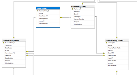
FIGURE 3-12: Tables and relationships in the AdventureWorks database.
The AdventureWorks sample database does not come with SQL Server 2017. It must be downloaded and installed separately. The installation procedure is somewhat involved, so be sure to read the installation instructions thoroughly before attempting to install it.
There is a one-to-many relationship between SalesTerritory and Customer, a one-to-many relationship between SalesTerritory and SalesPerson, and a one-to-many relationship between SalesPerson and SalesPersonQuotaHistory. The AdventureWorks database is fairly large and contains multiple schemas. All the tables in Figure 3-12, plus quite a few more, are contained in the Sales schema. You might have questions about the AdventureWorks business, as modeled by this database. In the following section, I build a query to answer one of those questions.
A typical query
Suppose you want to know if any of AdventureWorks’s salespeople are promising more than AdventureWorks can deliver. You can get an indication of this by seeing which salespeople took orders where the ShipDate was later than the DueDate. An SQL query will give you the answer to that question.
SELECT SalesOrderID
FROM AdventureWorks.Sales.Salesperson, AdventureWorks.Sales.SalesOrderHeader
WHERE SalesOrderHeader.SalesPersonID = SalesPerson.SalesPersonID
AND ShipDate > DueDate ;
Figure 3-13 shows the result. The result set is empty. There were no cases where an order was shipped after the due date.

FIGURE 3-13: SQL Server 2008 Management Studio execution of an SQL query.
The execution plan
Click on the Display Estimated Execution Plan icon to show what you see in Figure 3-14. An index scan, a clustered index scan, and a hash match consumed processor cycles, with the clustered index scan on SalesOrderHeader taking up 85 percent of the total time used. This shows that a lot more time is spent dealing with the SalesOrderHeader table than with the SalesPerson table. This makes sense, as I would expect there to be a lot more sales orders than there are sales people. This plan gives you a baseline on performance. If performance is not satisfactory, you can rewrite the query, generate a new execution plan, and compare results. If the query will be run many times, it is worth it to spend a little time here optimizing the way the query is written.
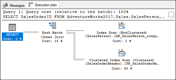
FIGURE 3-14: The execution plan for the delivery time query.
Running the Database Engine Tuning Advisor
Although the answer to this query came back pretty fast, one might wonder whether it could have been faster. Executing the Database Engine Tuning Advisor may find a possible improvement. Run it to see. You can select the Database Engine Tuning Advisor from the Tools menu. After naming and saving your query, specify the AdventureWorks2017 database in the Tuning Advisor and then (for the Workload file part), browse for the file name that you just gave your query. Once you have specified your file, click the Start Analysis button. The Tuning Advisor starts chugging away, and eventually displays a result.
Wow! The Tuning Advisor estimates that the query could be speeded up by 93 percent by creating an index on the SalesOrderHeader column, as shown in Figure 3-15.
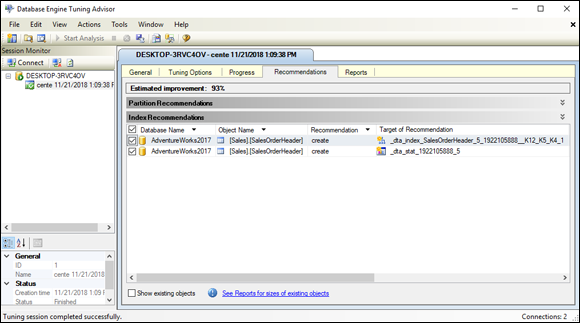
FIGURE 3-15: The recommendations of the Database Engine Tuning Advisor.