
Introduction
Abstract
This introductory chapter gives a general view on sensors. In the first section, the sensor’s functionality, sensor nomenclature, and global properties are presented, as a prelude to a more in-depth discussion about sensor performance and operation principles in subsequent chapters. According to the amount of information the output signal may contain, three categories of sensor are distinguished and each briefly discussed: binary, analogue, and image sensors. The latter category comprises optical, acoustic, and tactile image sensors. The second section presents a general approach to the selection process of sensors for a specified application. The last section introduces a platform for sensor architectures in an embedded environment and serves as the basis for the specific embedded sensing solutions discussed in the ensuing chapters.
Keywords
Transducer; sensor; actuator; proximity sensor; reed switch; imaging; sensor nomenclature; embedded sensing
Worldwide, sensor development is a fast growing discipline. Today’s sensor market offers thousands of sensor types, for almost every measurable quantity, for a broad area of applications, and with a wide diversity in quality. Many research groups are active in the sensor field, exploring new technologies, investigating new principles and structures, aiming at reduced size and price, at the same or even better performance.
System engineers have to select the proper sensors for their design, from an overwhelming volume of sensor devices and associated equipment. A well-motivated choice requires thorough knowledge of what is available on the market, and a good insight in current sensor research to be able to anticipate forthcoming sensor solutions.
This introductory chapter gives a general view on sensors—their functionality, the nomenclature, and global properties—as a prelude to a more in-depth discussion about sensor performance and operation principles.
1.1 Sensors in mechatronics
1.1.1 Definitions
A transducer is an essential part of any information processing system that operates in more than one physical domain. These domains are characterized by the type of quantity that provides the carrier of the relevant information. Examples are the optical, electrical, magnetic, thermal, and mechanical domains. A transducer is that part of a measurement system that converts information about a measurand from one domain to another, ideally without information loss.
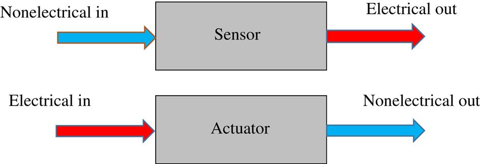
A transducer has at least one input and one output. In measuring instruments, where information processing is performed by electrical signals, either the output or the input is of electrical nature (voltage, current, resistance, capacitance, and so on), whereas the other is a nonelectrical signal (displacement, temperature, elasticity, and so on). A transducer with a nonelectrical input is an input transducer, intended to convert a nonelectrical quantity into an electrical signal in order to measure that quantity. A transducer with a nonelectrical output is called an output transducer, intended to convert an electrical signal into a nonelectrical quantity in order to control that quantity. So, a more explicit definition of a transducer is an electrical device that converts one form of energy into another, with the intention of preserving information.
According to common terminology, these transducers are also called sensor and actuator, respectively (Fig. 1.1). So, a sensor is an input transducer and an actuator is an output transducer. It should be noted, however, that this terminology is not standardized. In literature other definitions are found. Some authors make an explicit difference between a sensor and a (input) transducer, stressing a distinction between the element that performs the physical conversion and the complete device—for instance, a strain gauge (the transducer) and a load cell (the sensor) with one or more strain gauges and an elastic element.
Attempts to standardize terminology in the field of metrology have resulted in the Vocabulaire International de Métrologie (VIM) [1]. According to this document a transducer is a device, used in measurement, that provides an output quantity having a specified relation to the input quantity. The same document defines a sensor as the element of a measuring system that is directly affected by a phenomenon, body, or substance carrying a quantity to be measured.
Modern sensors not only contain the converting element but also part of the signal processing (analogue processing such as amplification and filtering, AD conversion, and digital processing). Many of such sensors have the electronics integrated with the transducer part onto a single chip. Present-day sensors may have a bus-compatible output, implying full signal conditioning on board, or include transmission electronics within the device, for instance, for biomedical applications.
Signal conditioning may be included:
- • to protect the sensor from being loaded or to reduce loading errors;
- • to match the sensor output range to the input range of the analog to digital converter (ADC);
- • to enhance the S/N (signal-to-noise ratio) prior to further signal processing;
- • to generate a digital, bus-compatible electrical output; or
- • to transmit measurement data for wireless applications.
In conclusion, the boundaries between sensor and transducer as proclaimed in many sensor textbooks are disappearing or losing their usefulness: the user buys and applies the sensor system as a single device, with a nonelectrical input and an electrical output (e.g., an analogue signal, a microprocessor compatible digital signal, or a radio signal).
1.1.2 Sensor development
Sensors provide the essential information about the state of a (mechatronic) system and its environment. This information is used to execute prescribed tasks, to adapt the system properties or operation to the (changing) environment or to increase the accuracy of the actions to be performed.
Sensors play an important role not only in mechatronics but also in many other areas. They are widely applied nowadays in all kind of industrial products and systems. A few examples are as follows:
and many other areas where the introduction of sensors has increased dramatically the performance of instruments, machines, and products.
The world sensor market is still growing substantially. The worldwide sensor market offers over 100,000 different types of sensors. This figure not only illustrates the wide range of sensor use but also the fact that selecting the right sensor for a particular application is not a trivial task. Reasons for the increasing interest in sensors are as follows:
- • Reduced prices: the price of sensors not only depends on the technology but also on production volume. Today, the price of a sensor runs from several ten thousands of euros for single pieces down to a few eurocents for a 100 million volume.
- • Miniaturization: the IC-compatible technology and progress in micromachining technology are responsible for this trend [2–4]. Pressure sensors belong to the first candidates for realization in silicon (early 1960s). Micro-ElectroMechanical Systems (MEMS) are gradually taking over many traditionally designed mechanical sensors [5–7]. Nowadays, solid-state sensors (in silicon or compatible technology) for almost every quantity are available, and there is still room for innovation in this area [8,9].
- • Smart sensing: the same technology allows the integration of signal processing and sensing functions on a single chip. Special technology permits the processing of both analogue and digital signals (“mixed signals”), resulting in sensor modules with (microprocessor compatible) digital output.
Popular MEMS sensors are accelerometers and gyroscopes. A MEMS accelerometer can be made completely out of silicon, using micromachining technology. The seismic mass is connected to the substrate by thin, flexible beams, acting as a spring. The movement of the mass can be measured by, for instance, integrated piezoresistors positioned on the beam at a location with maximum deformation (Chapter 4) or by a capacitive method (Chapter 5).
In mechatronics, mainly sensors for the measurement of mechanical quantities are encountered. The most frequent sensors are for displacement (position) and force (pressure), but many other sensor types can be found in a mechatronic system.
Many sensors are commercially available and can be added to or integrated into a mechatronic system. This approach is preferred for systems with relatively simple tasks and operating in a well-defined environment, as commonly encountered in industrial applications. However, for more versatile tasks and specific applications, dedicated sensor systems are required, which are often not available. Special designs, further development or even research are needed to fulfill specific requirements, for instance, with respect to dimensions, weight, temperature range, and radiation hardness.
1.1.3 Sensor nomenclature
In this book, we follow a strict categorization of sensors according to their main physical principle. The reason for this choice is that sensor performance is mainly determined by the physics of the underlying principle of operation. For example, a position sensor can be realized using resistive, capacitive, inductive, acoustic, and optical methods. The sensor characteristics are strongly related to the respective physical transduction processes. However, a magnetic sensor of a particular type could be applied as, for instance, a displacement sensor, a velocity sensor, or a tactile sensor. For all these applications the performance is limited by the physics of this magnetic sensor.
Apparently, position and movement lead the list of measurement quantities. Common parlance contains many other words for position parameters. Often, transducers are named after these words. Here is a short description of some of these transducers.
| Distance sensor | Measures the length of the straight line between two defined points |
| Position sensor | Measures the coordinates of a specified point of an object in a specified reference system |
| Displacement sensor | Measures the change of position relative to a reference point |
| Range sensor | Measures in a 3D space the shortest distance from a reference point (the observer) to various points of object boundaries in order to determine their position and orientation relative to the observer or to get an image of these objects |
| Proximity sensor | (1) Determines the sign (positive or negative) of the linear distance between an object point and a fixed reference point; also called a switch |
| (2) A contact-free displacement or distance sensor for short distances (down to zero) | |
| Level sensor | Measures the distance of the top level of a liquid or granular substance in a container with respect to a specified horizontal reference plane |
| Angular sensor | Measures the angle of rotation relative to a reference position |
| Encoder | Displacement sensor (linear or angular) containing a binary coded ruler or disk |
| Tilt sensor | Measures the angle relative to the earth’s normal |
| Tachometer | Measures rotational speed |
| Vibration sensor | Measures the motion of a vibrating object in terms of displacement, velocity, or acceleration |
| Accelerometer | Measures acceleration |
Transducers for the measurement of force and related quantities are as follows:
| Pressure sensor | Measures pressure difference, relative to either vacuum (absolute pressure), a reference pressure, or ambient pressure |
| Force sensor | Measures the (normal and/or shear) force exerted on the active point of the transducer |
| Torque sensor | Measures torque (moment) |
| Force–torque sensor | Measures both forces and torques (up to six components) |
| Load cell | Force or pressure sensor, for measuring weight |
| Strain gauge | Measures linear relative elongation (positive or negative) of an object, caused by compressive or tensile stress |
| Touch sensor | Detects the presence or (combined with a displacement sensor) the position of an object by making mechanical contact |
| Tactile sensor | Measures 3D shape of an object by the act of touch, either sequentially using an exploring touch sensor or instantaneously by a matrix of force sensors |
Many transducers have been given names according to their operating principle, construction, or a particular property. Examples are as follows:
| Hall sensor | Measures magnetic field based on the Hall effect, after the American physicist Edwin Hall (1855–1938) |
| Coriolis mass flow sensor | Measures mass flow of a fluid by exploiting the Coriolis force exerted on a rotating or vibrating channel with that fluid; after Gustave-Gaspard de Coriolis, French scientist (1792–1843) |
| Gyroscope, gyrometer | A device for measuring angle or angular velocity, based on the gyroscopic effect occurring in rotating or vibrating structures |
| Eddy current sensor | Measures short range distances between the sensor front and a conductive object using currents induced in that object due to an applied AC magnetic field; also used for defect detection |
| LVDT | Or Linear Variable Displacement Transformer, a device that is basically a voltage transformer, with linearly movable core |
| NTC | Short for temperature sensor (especially thermistor) with Negative Temperature Coefficient |
Some sensors use a concatenation of transduction steps. A displacement sensor, combined with a spring, can act as a force sensor. In combination with a calibrated mass, a displacement sensor can serve as an accelerometer. The performance of such transducers not only depends on the primary sensor but also on the added components: in the examples above the spring compliance and the seismic mass, respectively.
Information about a particular quantity can also be obtained by calculation using relations between quantities. The accuracy of the result depends not only on the errors in the quantities that are measured directly but also on the accuracy of the parameters in the model that describes the relation between the quantities involved. For instance, in an acoustic distance measurement the distance is calculated from the measured time-of-flight (ToF; with associated errors) and the sound velocity. An accurate measurement result requires knowledge of the acoustic velocity of the medium at the prevailing temperature.
Some variables can be derived from others by electronic signal processing. Speed and acceleration can be measured using a displacement sensor, by differentiating its output signal once or twice, respectively. Conversely, by integrating the output signal of an accelerometer a velocity signal is obtained and, by a second integration, a position signal. Obviously, the performance of the final result depends on the quality of the signal processing. The main problem with differentiation is the increased noise level (in particular in the higher frequency range), and integration may result in large drift due to the integration of offset.
1.1.4 Sensors and information
According to the amount of information a sensor or sensing system offers, three groups of sensors can be distinguished: binary sensors, analogue sensors, and image sensors. Binary sensors give only one bit of information but are very useful in mechatronics. They are utilized as end stops, as event detectors and as safety devices. Depending on their output (0 or 1), processes can be started, terminated, or interrupted. The binary nature of the output makes them highly insensitive to electrical interference.
Analogue sensors are used for the acquisition of metric information with respect to quantities related to distance (e.g., relative position, linear and angular velocity, and acceleration), force (e.g., pressure, gripping force, and bending), or others (e.g., thermal, optical, mechanical, electrical, or magnetic properties of an object). A wide variety of industrial sensors for these purposes are available.
The third category comprises image sensors, intended for the acquisition of information related to structures and shapes. Depending on the application, the sensor data refer to one-, two-, or three-dimensional images. The accuracy requirements are less severe compared to the sensors from the preceding category, but the information content of their output is much larger. As a consequence, the data acquisition and processing for such sensors are more complex and more time consuming.
The next sections present some general aspects of sensors, following the categorization in binary, analogue, and image sensors as introduced before. Actually, the section serves as a general overview of the sensors and sensing systems which are discussed in more detail in subsequent chapters. Details on physical background, specifications, and typical applications are left for those chapters. Here, the differences in approach are highlighted and their consequences for the applicability in mechatronic systems are emphasized.
1.1.4.1 Binary sensors
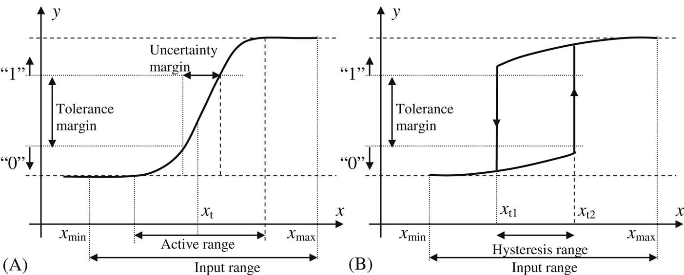
A binary sensor has an analogue input and a two-state output (0 or 1). It converts the (analogue) input quantity to a one bit output signal. These sensors are also referred to as switches or detectors. They have a fixed or an adjustable threshold level xt (Fig. 1.2A). In fact, there are essentially two levels, marking the hysteresis interval (Fig. 1.2B). Any analogue sensor can be converted to a binary sensor by adding a Schmitt trigger (comparator with hysteresis, Appendix C.5). Although hysteresis lowers the accuracy of the threshold detection (down to the hysteresis interval), it may help reducing unwanted bouncing due to noise in the input signal.
Most binary sensors measure position. Binary displacement sensors are also referred to as proximity sensors. They react when a system part or a moving object has reached a specified position. Two major types are the mechanically and the magnetically controlled switches.
Mechanically controlled switches are actually touch sensors. They are available in a large variety of sizes and constructions; for special conditions there are waterproof and explosion-proof types; for precision measurements there are switches with an inaccuracy less than ±1 μm and a hysteresis interval in the same order, guaranteed over a temperature range from −20°C to 75°C. Another important parameter of a switch is the reliability, expressed in the minimum number of commutations. Mechanical switches have a reliability of about 106.
A reed switch is a magnetically controlled switch: two magnetizable tongues or reeds in a hermetically closed encapsulation filled with an inert gas. The switch is normally off; it can be switched on mechanically by a permanent magnet approaching the sensor. Reed switches have good reliability: over 107 commutations at a switching frequency of 50 Hz. A disadvantage is the bouncing effect, the chattering of the contacts during a transition of state. Reed switches are applied in various commercial systems, from cars (monitoring broken lights, level indicators) to electronic organs (playing contacts), to telecommunication devices and testing and measurement equipments. In mechatronic systems, they act as end-of-motion detectors, touch sensors, and other safety devices. The technical aspects are described in Chapter 6 on inductive and magnetic sensors.
The drawbacks of all mechanical switches are a relatively large switch-on time (for reed switches typically 0.2 ms) and wear. This explains the growing popularity of electronic switches, such as optically controlled semiconductors and Hall plates. There is a wide range of binary displacement sensors on the market, for a variety of distances and performance. Table 1.1 presents a concise overview of specifications.
Table 1.1
| Type | Working range | Response time | Reproducibility |
|---|---|---|---|
| Mechanical | 0 (contact) | ±1 μm | |
| Reed switch | 0–2 cm | 0.1 ms (on) | |
| Optical | 0–2/10/35 ma | 500 Hz/1 ms | 10 cm |
| Inductive | 0–50 cm | 1 ms | 1 cm |
| Capacitive | 0–40 mm | 1 ms | 1 mm |
| Magnetic | 0–100 mm | 10 μm |

aReflection from object/reflector/direct mode.
All these sensors except for the mechanical switch operate essentially contact-free. Obviously, the optical types have the widest distance range. The optical, inductive, and capacitive types are essentially analogue sensors, with adjustable threshold levels. The specifications include interface and read-out electronics. In particular, the response time of the sensor itself may be much better than the value listed in the table. Accuracy data include hysteresis and apply for the whole temperature range (maximum operating temperature range 70°C typical).
1.1.4.2 Analogue sensors
There is an overwhelming number of analogue sensors on the market, for almost any physical quantity, and operating according to a diversity of physical principles. In mechatronics, the major measurement quantities of interest are linear and angular displacement, their time derivatives (velocity and acceleration), and force (including torque and pressure). These and many other sensors will be discussed in more detail in later chapters.
1.1.4.3 Image sensors
Imaging is a powerful method to obtain information about geometrical parameters of objects with a complex shape. The 3D object or a complete scene is transformed to a set of data points representing the geometrical parameters that describe particular characteristics of the object, for instance, its pose (position and orientation in space), dimensions, shape, or identity. An essential condition in imaging is the preservation of the required information. This is certainly not trivial: photographic and camera pictures are 2D representations of a 3D world, and hence much information is lost by the imaging process.
Three basic concepts for image acquisition are depicted schematically in Fig. 1.3. In the first method the scene to be imaged is scanned point by point by some mechanical means (e.g., a mirror on a stepping motor) or electronically (for instance, with phased arrays). Such an imaging system is often referred to as a range finder: it yields distance information over an angular range determined by the limits of the scanning mechanism. The output is a sequential data stream containing 3D information about the scene: depth data from the scanning sensor and angular data from the scanning mechanism. Although the data points are three-dimensional, information is obtained only about the surface boundary range and only that part of the surface that is connected to the sensor system by a line of direct sight. Therefore range data are sometimes called 2.5D data. In Fig. 1.3A, the sensor and scanning mechanism are presented as a single device. Most scanning systems consist of several parts, for instance, a fixed transmitter and receiver and one or more rotating mirrors or reflectors. Sometimes the transmitter, the receiver, or both are mounted on the scanning device. Although the scanning method is slow, it requires only a single sensor which can therefore be of high quality.
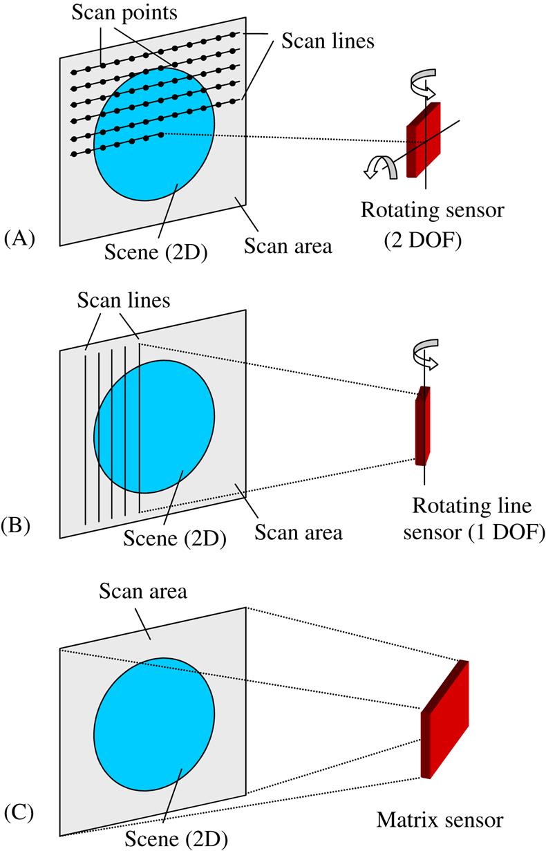
In the second method (Fig. 1.3B) the scene is scanned line by line, again using some mechanical scanning device. Each line is projected onto an array of sensors (in the optical domain for instance a diode array). The sensor array may include electronic scanning to process the data in a proper way. Nevertheless, the mechanical scanning mechanism operates in only one direction, which increases the speed of image formation and lowers construction complexity as compared to point-wise scanning.
The third method (Fig. 1.3C) involves the projection of the unknown image on a 2D matrix of point sensors. This matrix is electronically scanned for serial processing of the data. Since all scanning is performed in the electronic domain, the acquisition time is short. The best known imaging device is the CCD matrix camera (Charge Coupled Device). It has the highest spatial resolution of all matrix imagers.
Considering the nature of the various possible information carriers, there are at least three candidates for image acquisition: light, (ultra)sound and contact force. All three are being used in both scanning and projection mode. Most popular is the CCD camera as imager for exploring and analyzing the work space of a mechatronic system or a robot’s environment. However, in numerous applications the camera is certainly not the best choice.
The acquisition of an image is just the first step in getting the required information; data processing is another important item. There is a striking difference between (camera based) vision and nonvision data processing. The main problem of the CCD camera is the provision of superfluous data. The first step in image processing is, therefore, to get rid of all irrelevant data in the image. For instance, a mere contour might be sufficient for proper object identification; the point is how to find the right contour. However, most nonvision imagers suffer from a too-low-resolution. Here the main problem is the extraction of information from the low-resolution image and—in the case of scanning systems—from other sensors. In all cases, model-driven data processing is required to be able to arrive at proper conclusions about features of the objects or the scene under test.
1.1.4.4 Optical imaging
Most optical imaging systems applied in mechatronics and robotics use a camera (CCD-type or CMOS) and a proper illumination of the scene. The image (or a pair of images or even a sequence when 3D information is required) is analyzed by some image processing algorithm applied to the intensity and color distribution in the image. Particular object features are extracted from particular patterns in light intensity in the image. Position information is derived from the position of features in the image, together with camera parameters (position and orientation, focal length).
Specified conditions for getting a proper image must be fulfilled: an illumination that yields adequate contrast and no disturbing shadows and a camera set-up with a full view on the object or the scene and with a camera that has a sufficiently high resolution, so as not to lose relevant details. Obviously, a 2D image shows only a certain prospect of the object, never a complete view (self-occlusion). In case of more than one object, some of them could be (partially) hidden behind others (occlusion), a situation that makes the identification much more difficult.
Even in the most favorable situation, the image alone does not reveal enough information for the specified task. Besides a proper model of the object, we need a model of the imaging process: position and orientation of the camera(s), camera parameters like focal length, and the position of the light source(s) with respect to the object and camera. All of these items determine the quality of the image from which features are to be extracted. The pose of the object in the scene can be derived from the available information and knowledge of the imaging system.
Many algorithms have been developed to extract useful features from an image that is built up of thousands of samples (in space and time) described by color parameters, gray-tone values or just bits for black and white images. The image is searched for particular combinations of adjacent pixels such as edges, from which region boundaries are derived. Noise in the image may disturb this process, and special algorithms have been developed to reduce its influence. The result is an image that reveals at least some characteristics of the object. For further information on feature extraction the reader is referred to the literature on computer vision and image processing.
1.1.4.5 Acoustic imaging
The interest in acoustic waves for imaging is steadily growing, mainly because of the low cost and simple construction of acoustic transducers. The suitability of acoustic imaging has been proved in medical, geological, and submarine applications. Applications in mechatronics have, however, some severe limitations going back to ultrasonic wave propagation in air (where most mechatronic systems operate). Despite these limitations, detailed in Chapter 9, many attempts are being made to improve the accuracy and applicability of acoustic measurement systems, in particular as they are applied to distance measurement and range finding.
The most striking drawback of acoustic imaging is the low spatial resolution, due to the diverging beam of acoustic transducers. The directivity of the transducers can be improved by increasing the ratio between the diameter and the wave length. Even at medium frequencies (i.e., 40 kHz), this results in rather large devices. An alternative method is the use of an array of simultaneously active acoustic elements. Due to interference, the main beam (in the direction of the acoustic axis) is narrowed. Further, the direction of this beam can be electronically controlled by variation of the phase shift or time delay between the elements of the array. This technique, known as phased arrays, applies to transmitters as well as receivers.
The recognition of shapes requires a set of distance sensors or scanning with a single sensor, according to one of the principles in Fig. 1.3. The shape follows from a series of numerical calculations (see, for instance, Refs. [10,11]).
Instead of geometric models for use in object recognition, other models may be used. An example of such a different approach is shown schematically in Fig. 1.4. An acoustic signal (the stimulus) is transmitted toward the object. The shape of the echo pattern (the response) is determined by the object’s shape and orientation. In a learning phase, echo patterns of all possible objects are stored in computer memory. They can be considered acoustic signatures of the objects. The echo pattern from a test object belonging to the trained set is matched to each of the stored signatures. Using a minimum distance criterion reveals the best candidate [12]. Evidently, the test conditions should be the same as during the learning phase: a fixed geometry and a stable stimulus are required.
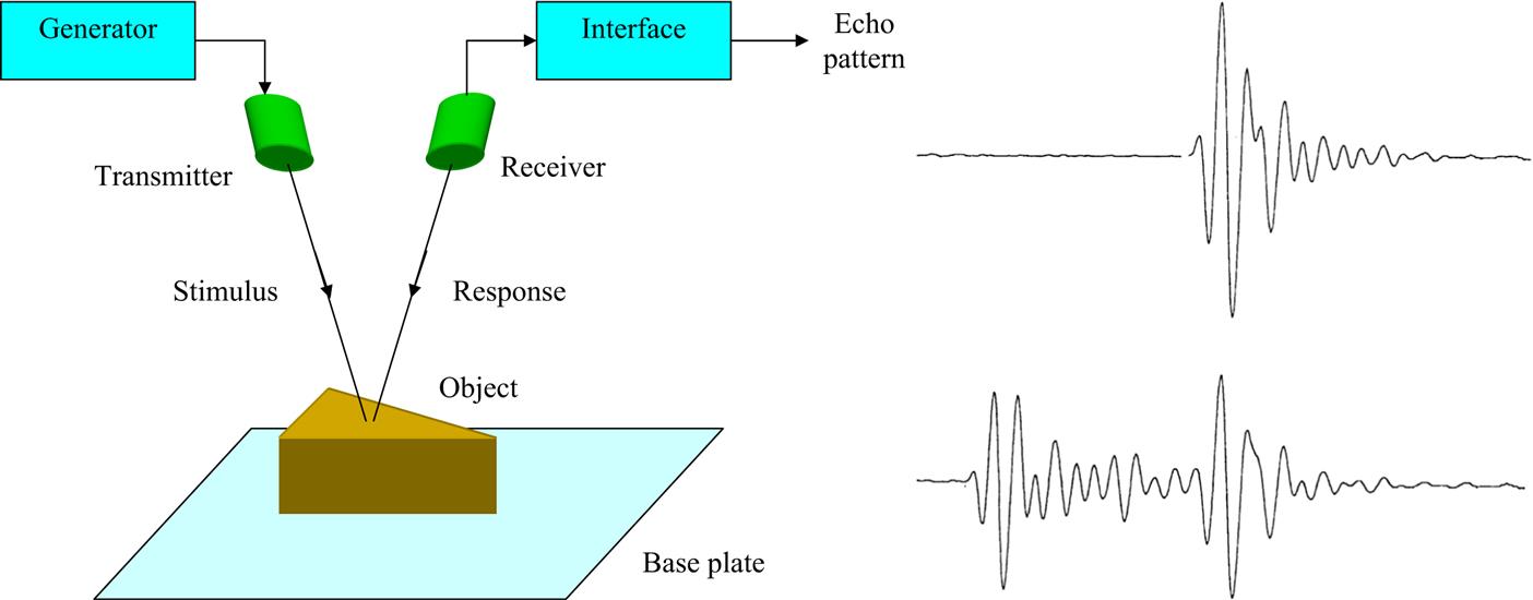
The comparison process may be performed either in the frequency domain or in the time domain. With this simple technique, it is possible to distinguish between objects whose shapes or orientations (normal vs upside-down position) are quite different. With an adaptive stimulus and a suitable algorithm, even small defects in an object can be detected by ultrasonic techniques. Under certain conditions, very small object differences can be detected, for instance, between sides of a coin [13].
1.1.4.6 Tactile imaging
In contrast to optical and acoustic imaging, tactile imaging is performed by mechanical contact between sensor and object. Making contact has advantages as well as disadvantages. Disadvantages are the mechanical load of the object (it may move or be pressed) and the necessity of moving the sensor actively toward the object. Advantages of tactile imaging include the possibility of acquiring force-related information (for instance, touching force and torque) and mechanical properties of the object (e.g., elasticity, resilience, and surface texture). Another advantage over optical imaging is the insensitivity to environmental conditions. This versatility of a tactile sensor makes it very attractive for control purposes, especially in assembly processes. Moreover, tactile and vision data can be fused, to benefit from both modalities.
In robotics, tactile imaging is mostly combined with the gripping action. For in-line control the tactile sensor should be incorporated into the gripper of the robot, allowing simultaneous force distribution and position measurements during the motion of the gripper. This permits continuous force control as well as position correction.
In inspection systems (like coordinate measuring machines), the object under test is scanned mechanically by a motion mechanism, with a touch sensor as the end effector. The machine is controlled to follow a path along the object, while keeping the touch force at a constant value. Position data follow from back transformation of the tip (sensor) coordinates to world coordinates. The scanning is slow but can be very accurate, down to 10 nm in three dimensions.
1.2 Selection of sensors
Choosing a proper sensor is certainly not a trivial task. First of all, the task that is to be supported by one or more sensors needs to be thoroughly analyzed and all possible strategies to be reviewed. Potential sensors should be precisely specified, including environmental conditions and mechanical and electrical constraints. If commercial sensors can be found that satisfy the requirements, purchase is recommended. Special attention should be given to interface electronics (in general available as separate units, but rarely adequate for newly developed mechatronic systems). If the market does not offer the right sensor system, such a system may be assembled from commercial sensor components and electronics. This book gives some physical background of most sensors, to help understand their operation, to assist in making a justified choice, or to provide knowledge for assembling particular sensing systems.
Sensor selection is based on satisfying requirements; however, these requirements are often not known precisely or in detail, in particular when the designer of the system and its user are different persons. The first task of the designer, therefore, is to get as much information as possible about the future applications of the system, all possible conditions of operation, the environmental factors, and the specifications, with respect to quality, physical dimensions, and costs.
The list of demands should be exhaustive. Even when not all items are relevant, they must be indicated as such. This will leave more room to the designer and minimizes the risk of having to start all over again. The list should be made in a way that enables unambiguous comparison with the final specifications of the designed system. Once the designer has a complete idea about the future use of the system, the phase of the conceptual design can start.
Before thinking about sensors, the measurement principle first has to be considered. For the instrumentation of each measurement principle, the designer has a multitude of sensing methods at his disposal. For the realization of a particular sensor method, the designer has to choose the optimal sensor component and sensor type from a vast collection of sensors offered by numerous sensor manufacturers.
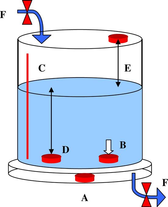
This design process is illustrated by an example of a measurement for just a single, static quantity: the amount of fluid in a container (for instance, a drink dispenser). The first question to be answered is, in what units the amount should be expressed: volume or mass? This may influence the final selection of the sensor. Fig. 1.5 shows various measurement principles in a schematic way:
- A: the tank is placed on a balance, to measure its total weight;
- B: a pressure gauge on the bottom of the tank;
- C: a gauging-rule from top to bottom with electronic read-out;
- D: level detector on the bottom, measuring the column height;
- E: level detector from the top of the tank, measuring the height of the empty part;
- F: (mass or volume) flow meters at both inlet and outlet.
Obviously, many more principles can be found to measure a quantity that is related to the amount of fluid in the reservoir.
In the conceptive phase of the design as many principles as possible should be considered, even unconventional ones. Based on the list of demands, it should be possible to find a proper candidate principle from this list, or at least to delete many of the principles, on an argued base. For instance, if the tank contains a corrosive fluid, a noncontact measurement principle is preferred, putting principles B, C, and D on a lower position in the list.
Further, for very large tanks, method A can possibly be eliminated because of high costs. The conceptual design ends up with a set of principles with pros and cons, ranked according to the prospects of success.
After having specified a list of candidate principles, the next step is to find a suitable sensing method for each of them. In the example of Fig. 1.5, we will further investigate principle E, a level detector placed at the top of the tank. It should be noted that from level alone the amount of liquid cannot be determined: the shape of the container should also be taken into account. Again, a list of the various possible sensor methods is made, as follows:
As in the conceptual phase, these methods are evaluated using the list of demands, so not only the characteristics of the sensing method but also the properties of the measurement object (e.g., kind of liquid and shape of tank) and the environment should be taken into account. For the tank system, the acoustic ToF method could be an excellent candidate because of its being contact free. In this phase, it is also important to consider methods to reduce such environmental factors as temperature. Ultimately, this phase concludes with a list of candidate sensing methods and their merits and demerits with respect to the requirements.
The final step is the selection of the components that make up the sensing system. Here a decision must be made between the purchase of a commercially available system and the development of a dedicated system. The major criteria are costs and time: both are often underestimated when development by one’s own is considered.
In this phase of the selection process, sensor specifications become important. Sensor providers publish specifications in data sheets or on the Internet. However, the accessibility of such data is still poor, making this part of the selection process critical and time consuming, in particular for nonspecialists in the sensor field.
Evidently, the example of the level sensor is highly simplified, whereas the selection process is usually not that straightforward. Since the sensor is often just one element in the design of a complex mechatronic system, close and frequent interaction with other design disciplines as well as the customer is recommended.
1.3 Embedded sensing
Sensors play a critical role in current developments in industry and the internet of things. They are more often than not referred to not just as the transducers converting physical signals to the electrical domain, but are discussed as complete systems. A “sensor node” in Industry 4.0 or in the Internet of things normally consists of an embedded, integrated system containing power, processing, means of communication and—eventually—the sensing element. Large amounts of data (big data) is generated using vast networks of smart sensor nodes measuring plant conditions, water quality or the weather—often with greater robustness, higher accuracy, or better resolution than conventional remote sensing technology can.
This means that for smart industry, internet of things and mechatronic applications, the possibilities for interfacing and (embedded) processing of sensor signals are almost as important in the selection criteria as the choice of a suitable physical transducer. To underline this importance, for every physical principle a number of embedded processing examples will be discussed. These are by no means meant as design guidelines or full-blown recipes, but aim to give insight in the possibilities, offer an option for learning, and can be used as starting point for further design or development.
1.3.1 Interfacing, conditioning, processing
The sensors discussed in this book are mainly transducers translating quantities in a physical domain into the electrical domain. The discussed applications (in mechatronics) are largely not only in the electrical signal domain, but in the digital domain as well. A transducer converts or transforms information (thus power) from one domain into the other. Also the act of observing changes the observed (not only true in quantum mechanics). An ideal transducer converts as little energy as possible in order not to have an impact on the measurand. This means that the converted electrical measurement signals are typically small and need additional conditioning such as amplification, offset reduction, and linearization. This can be achieved in many ways: by clever sensor design, by adding conditioning circuitry, or by processing the data in the digital domain. For processing data in the digital domain, it is necessary that data have been converted from the electrical domain into a digital representation, typically by an analog to digital conversion. Alternatively, sensors can also be designed in such a fashion that their primary output is already in the digital domain: incremental encoders or (especially) absolute optical encoders give their output in digital “steps” or “bits,” see Chapter 7.
This approach (schematically shown in Fig. 1.6) can also be recognized in most of the common (household) digital sensing systems such as digital fever thermometers or bathroom scales. The circuits for conditioning, conversion, and processing are usually condensed to a single integrated circuit, usually outputting data on a small liquid crystal display.

For every type of transducer a number of strategies for interfacing accompanied by useful conditioning circuits exist. When eventually a voltage is generated that has a linear relation (preferably) or at least changes with the measurand, the work in the electrical domain can be considered done—and the signal can be converted to the digital domain (typically with ADC) for further processing and finally visualization and interpretation.
1.3.2 Platform for illustration
In order to illustrate interfacing options and (simple) processing algorithms a platform has been chosen which has become a de-facto standard in education and Do-It-Yourself (DIY) applications. The Arduino platform has been built around a number of members of Atmel AVR RISC (reduced instruction set) 8-bit microcontroller series. In recent years the family has been expanded to boards based on ARM, Intel x86 architecture, and many more. While there exist many more systems, embedded architectures, families, boards, etc, this choice has been made in the hope to provide accessible and reproducible examples which can be easily translated to a different system of choice.
The board which will be used for the experiments and examples discussed is the most common member of the Arduino family, the Arduino Uno (Fig. 1.7), which has been in development for more than 10 years, and not substantially changed, merely fine-tuned in the process.
This board consists of an ATmega328p microcontroller by Atmel running at 16 MHz, a small power section (linear 5 and 3.3 V regulators) and a separate ATmega8U2 microcontroller which is used as USB-CDC device for programming and communication. A single USB connection can be used for both programming the device (i.e., uploading new programs into the main controllers Flash memory) and communication with the device. Many more boards exist in the Arduino family using a large variety of communication and programming protocols such as JTAG, 1-wire debug, native USB and communication protocols such as Bluetooth, WIFI, LoraWAN, etc. but these are, although interesting for developing sensor nodes and networks, considered beyond the scope of understanding the basics necessary for embedded processing. A number of publications are referenced at the end of this chapter to act as starting points for more elaborate development.
1.3.3 Embedded control architecture
The ATmega328p controller which forms the heart of the discussed Arduino board is an 8-bit RISC microcontroller running at 16 MHz. The RISC implies that most of the low-level instructions can actually be processed in one clock cycle (which means 16,000,000 instructions per second). The controller has 4 kB of RAM memory, 32 kB of Flash memory for program storage, and 1 kB of EEPROM. It contains a number of timers which can be used for interrupts or the generation of pulse width modulation signals and hardware support for a number of communication protocols and standards (SPI, I2C), and a general purpose synchronous serial interface (UART).
For embedded sensing one of the most relevant devices in the controller is the ADC. The board that is used has a 6-channel 10 bit AD converter which in the normal configuration (single channel) can take a sample in 100 μs (so a maximum sampling rate of 10 kHz), depending on how the sampling routine is configured and implemented. Note that this is largely caused by the implementation of the functions (“analogRead()”) in the Arduino environment and libraries. It is possible to achieve higher sampling rates using different implementations in code, see Appendix D for examples.
The reference voltage for the internal AD converter can be set to an internal 1.1 V reference, the default 5.0 V (supply) reference, or an external reference (see Appendix D).
The input pins that can be used for AD conversion (the controller has just one AD converter and a 6-channel multiplexer) can be used as general purpose input or output pins as well. It is also possible to use an internal pull-up resistor on every input pin, thus (in simple cases) eliminating the need for additional components for interfacing sensors.
1.3.4 Developing applications
Software for the Arduino board can be written on an integrated development environment (IDE) running on a host computer. Versions of this IDE exist for many operating systems (Windows, Linux, and Mac OSX) and can be downloaded freely (the sources are licensed as GPL) from the Arduino.cc website. The IDE (shown in Fig. 1.8) is written in java and relies on the GNU AVR-GCC compiler and AVR-dude projects for respectively compiling code (C++) and programming the devices.
In many applications for design and education, the input of a sensor is compared with a certain threshold value, and action is taken accordingly. Goal of the illustrated examples is to get a step further, and translate the obtained sensor signals back to meaningful SI units.
The power of embedded control, even by relatively (computationally) simple devices as 8-bit AVR microcontrollers, has been shown by the development in the Maker/DIY community of 3D printers, quadcopters, and balancing vehicles. The real-time, low-level sensing and control (maintaining the heat in a print head, heading and altitude of the quadcopter, or the balance of a Segway) is in these examples carried out by the microcontroller, the overall (human in the) loop control by a host system or remote operator.
For the examples shown in this book a similar approach will be taken. After interfacing, conditioning and processing the signals in the embedded platform, recording, visualization, and interpretation needs to take place as well.
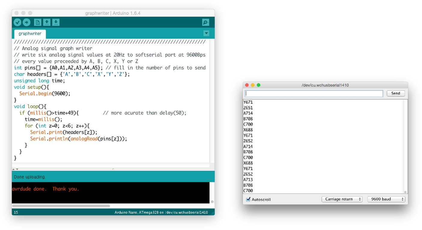
Although the Arduino IDE contains a number of tools for elementary visualization and recording of data (a serial monitor tool and a rudimentary graph writer), a different tool is introduced here for recording, visualizing, and processing the sensor data on a host PC system. The platform used for a number of simple illustrating examples is aptly named “Processing,” freely obtainable for multiple operating systems from the website of Processing (http://processing.org). The IDEs for both processing and Arduino have a very similar look and feel. Fig. 1.9 shows the IDE of Processing with a “graphwriter” example as discussed in Appendix D. They are by no means full-blown environments for industrial product development, but are specifically designed to create small tests, proof-of-concepts, and working prototypes. Hence programs are denoted as “sketches.”

Starting in Chapter 4 a number of examples of embedded sensing using the described Arduino board and IDE will be given. Besides these tools a conventional spreadsheet tool (such as Microsoft Excel, Apple iWork’s “Numbers,” or LibreOffice Calc) will be used. Many examples exist for importing data and interfacing the board directly with environments such as MatLab or LabView. As said, the described tools are only used as simple examples to illustrate the possibilities of embedded sensing.
Much of the relevant information for getting started with embedded sensing, especially using the Arduino platform, can be found online. A good starting point is Arduino’s main website. References [14–16] provide a further introduction in the Arduino board and the DIY world which it revolves in. These books have a practical nature and contain step-by-step guidelines for installing the necessary software, connecting the board, connecting sensors as well as a basic introduction in practical electronics.