
Chapter 10. Staged and Packed Column Design
In previous chapters we learned how to determine the number of equilibrium stages and separation in distillation columns. In the first part of this chapter we discuss details of staged column design such as tray geometry, determination of column efficiency, calculation of column diameter, downcomer sizing, and tray layout. We start with a qualitative description of column internals and proceed to a quantitative description of efficiency prediction, determination of column diameter, sieve tray design, and valve tray design. In the second part (Sections 10.6 to 10.10) we discuss packed column design including selection of packing and determination of column length and diameter. New engineers are expected to do these calculations. The internals of distillation columns are usually designed under the supervision of experts with many years of experience.
This chapter is not a shortcut to becoming an expert. However, on completion of this chapter you should be able to finish a preliminary design of column internals for both staged and packed columns and discuss distillation designs intelligently with experts.
10.0 Summary—Objectives
In this chapter both qualitative and quantitative aspects of column design are discussed. After finishing this chapter you should be able to satisfy the following objectives:
1. Describe equipment used for staged distillation columns
2. Define different definitions of efficiency, predict overall efficiency, and scale-up efficiency from laboratory data
3. Determine diameter of sieve and valve tray columns, and adjust vapor flow rates to balance column diameters
4. Determine tray pressure drop terms for sieve and valve trays and design downcomers
5. Lay out a tray that will work
6. Describe parts of a packed column, and explain the purpose of each part
7. Use HETP method to design a packed column. Determine HETP from data
8. Calculate the required diameter of a packed column
9. Determine an appropriate range of operating conditions for a packed column
10. Select an appropriate design (sieve tray, valve tray, random packing, or structured packing) for a separation problem
11. Use a computer simulator for detailed design of tray distillation columns
10.1 Staged Column Equipment Description
A very basic picture of staged column equipment is presented in Chapter 3. In this section, a much more detailed qualitative picture is presented. This section is based on a series of articles and books by Kister (1980, 1981, 1992, 2005), the book by Ludwig (1997), and the chapter by Larson and Kister (1997). These sources should be consulted for more details.
Sieve trays, which are illustrated in Figure 3-7, are easy to manufacture and are inexpensive. Holes are punched or drilled (a more expensive process) in a metal plate. Considerable design information is available, and since designs are not proprietary, anyone can build a sieve tray column. Efficiency is good at design conditions. However, turndown (performance when operating below the designed flow rate) is relatively poor. This means that operation at significantly lower rates than the design condition will result in low efficiencies. For sieve plates, efficiency drops markedly for gas flow rates that are less than about 60% of the design value. Thus, these trays are not extremely flexible. Since sieve trays are easy to clean, they are very good in fouling applications and are the normal choice when solids are present. Sieve trays are a standard item in industry, but new columns are more likely to have valve trays (Kister, 1992).
Valve trays are designed to have better turndown properties than sieve trays, and thus, they are more flexible when feed rate varies. There are many different proprietary valve tray designs; one type is illustrated in Figure 10-1. Valve trays are similar to sieve trays in that they have decks with holes in them for gas flow and downcomers for liquid flow. However, the holes, which are quite large, are fitted with valves, which are covers that can move up and down as pressures of vapor and liquid change. Each valve has feet or a cage that restrict its upward movement. Round valves with feet are popular, but wearing of the feet can be a problem (Kister, 1990). At high vapor velocities, valves are fully open, providing a maximum slot for gas flow (see Figure 10-1). When gas velocity drops, some valves will close. This keeps gas velocity through the slot close to constant, which keeps efficiency close to constant and prevents weeping. An individual valve is stable only in fully closed or fully opened position. At intermediate velocities some valves on the tray will be open and some will be closed. Usually, valves alternate between the open and closed positions.
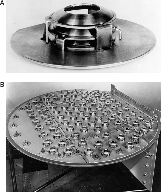
FIGURE 10-1. (A) Valve assembly for Glitsch A-1 valve, and (B) small Gitsch A-1 ballast tray; courtesy of Glitsch, Inc., Dallas, Texas
At the design vapor flow rate, valve trays have about the same efficiency as sieve trays. However, their turndown characteristics are generally better, and efficiency remains high as gas rate drops. Venturi valves have been designed to have a lower pressure drop than sieve trays. The lip of the hole faces upward to produce a Venturi opening, which minimizes pressure drop. However, the standard valve tray will have a higher pressure drop than sieve trays. Disadvantages of valve trays are they are about 20% more expensive than sieve trays (Glitsch, 1985), and they are more likely to foul or plug if dirty solutions are distilled.
Bubble-cap trays are illustrated in Figure 10-2. In a bubble cap there is a riser, or weir, around each hole. A cap with slots or holes is placed over this riser, and the vapor bubbles through these holes. This design is quite flexible and operates satisfactorily at very high and very low liquid flow rates. However, entrainment is about three times that of a sieve tray, and there is usually a significant liquid gradient across the tray. As a result tray spacing must be significantly greater than for sieve trays. Efficiencies are usually the same or less than for sieve trays, and turndown characteristics are often worse. The bubble cap has problems with coking, polymer formation, and high-fouling mixtures. Bubble-cap trays are approximately four times as expensive as valve trays (Glitsch, 1985). Very few new bubble-cap columns are being built. However, new engineers are likely to see older bubble-cap columns still operating. Many data are available for the design of bubble-cap trays. Since excellent discussions on the design of bubble-cap columns are available (Bolles, 1963; Ludwig, 1997), details are not given here.
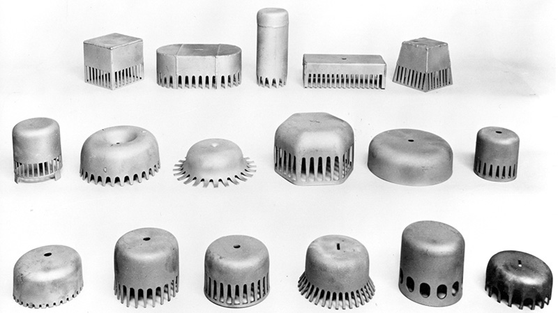
FIGURE 10-2. Different bubble-cap designs made by Glitsch, Inc., courtesy of Glitsch, Inc., Dallas, Texas
Perforated plates without downcomers look like sieve plates but with significantly larger holes. The plate is designed so that liquid weeps through holes simultaneously with vapor passing through the holes’ centers. This design eliminates the cost and space associated with downcomers. Its major disadvantage is that it is not robust. That is, if something goes wrong the column may not work at all instead of operating at a lower efficiency. These columns are usually designed by the company selling the system. Some design details are presented by Ludwig (1997).
10.1.1 Trays, Downcomers, and Weirs
In addition to choosing the type of tray, the designer must select the flow pattern on the trays and design weirs and downcomers. This section continues to be mainly qualitative.
The most common flow pattern on a tray is the crossflow pattern shown in Figure 3-7 and repeated in Figure 10-3A. This pattern works well for average flow rates and can be designed to handle suspended solids. Crossflow trays can be designed by the user on the basis of information in the open literature (Bolles, 1963; Fair, 1963, 1984, 1985; Kister, 1980, 1981, 1992; Ludwig, 1997), from information in company design manuals (Glitsch, 1974; Koch, 1982), and from any of the manufacturers of staged distillation columns. Design details for crossflow trays are discussed later.
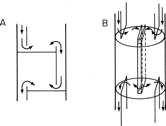
Multiple-pass trays are used in large-diameter columns with high liquid flow rates. Double-pass trays (Figure 10-3B) are common (Pilling, 2005). The liquid flow is divided into two sections (or passes) to reduce liquid gradient on the tray and to reduce downcomer loading. With even larger liquid loadings, four-pass trays are used; three-pass trays are not used because of liquid maldistribution (Kister et al., 2010; Pilling, 2005). Multipass trays are usually designed by experts, although preliminary designs can be obtained by following design manuals published by equipment manufacturers (Glitsch, 1974; Koch, 1982).
Which flow pattern is appropriate for a given problem? As the gas and liquid rates increase, the tower diameter increases. However, the ability to handle liquid flow increases with weir length, while the gas flow capacity increases with the square of the tower diameter. Eventually multiple-pass trays are required. A selection guide is given in Figure 10-4 (Huang and Hodson, 1958), but it is only approximate, particularly near the lines separating different types of trays.
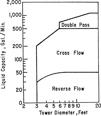
FIGURE 10-4. Selection guide for sieve trays, reprinted with permission from Huang and Hodson, Petroleum Refiner, 37 (2), 104 (1958), copyright 1958, Gulf Pub. Co.
Downcomers and weirs are very important for proper operation of staged columns, since they control liquid distribution and flow. A variety of designs are used, and four are shown in Figure 10-5 (Kister, 1980e, 1992). In small columns and pilot plants circular pipes (Figure 10-5A) are commonly used. The pipe may stick out above the tray floor to serve as the weir, or a separate weir may be used. In the Oldershaw design commonly used in pilot plants and university labs, the pipe is in the center of the sieve plate and is surrounded by holes. The most common design in commercial columns is the segmented vertical downcomer shown in Figure 10-5B. This type is inexpensive to build, easy to install, almost impossible to install incorrectly, and can be designed for a wide variety of liquid flow rates. If liquid-vapor disengagement is difficult, one of the sloped segmental designs shown in Figure 10-5C can be useful. These designs help retain the active area of the tray below. Unfortunately, they are more expensive and are easy to install backward. For very low liquid flow rates, the envelope design shown in Figure 10-5D is occasionally used.
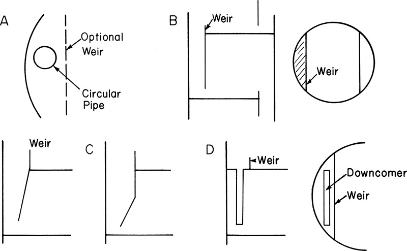
FIGURE 10-5. Downcomer and weir designs; (A) circular pipe, (B) straight segmental, (C) sloped downcomers, (D) envelope
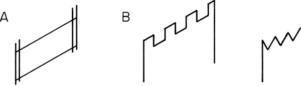
The simplest weir design is the straight horizontal weir from 2- to 4-in. high (Figures 3-7 and 10-5). This type is the cheapest but does not have the best turndown properties. The adjustable weir shown in Figure 10-6A is a very seductive design, since it appears to solve the problem of turndown. Unfortunately, if maladjusted, this weir can cause many problems such as excessive weeping or trays running dry, so it should be avoided. When flexibility in liquid rates is desired, one of the notched (or picket fence) weirs shown in Figure 10-6B works well (Pilling, 2005), and they are not much more expensive than a straight weir. Notched weirs are particularly useful with low liquid flow rates.
Trays, weirs, and downcomers need to be mechanically supported. These supports are illustrated in Figure 10-7 (Zenz, 1997). The trick is to adequately support the weight of the tray plus the highest possible liquid loading it can have without excessively blocking either the vapor flow area or the active area on the tray. As the column diameter increases, tray support becomes more critical. Ludwig (1997) and Kister (1980d, 1990, 1992) provide additional details.
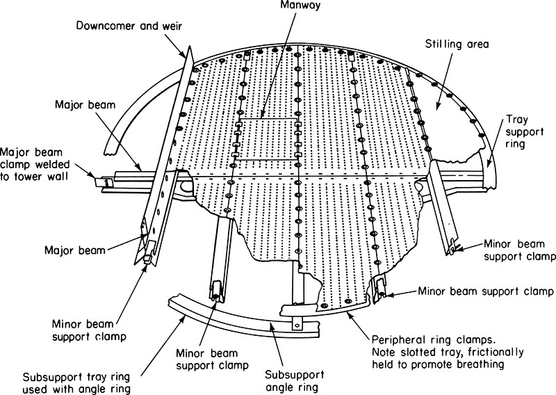
FIGURE 10-7. Mechanical supports for sieve trays from Zenz (1997). Reprinted with permission from Schweitzer, Handbook of Separation Techniques for Chemical Engineers, 3rd ed., copyright 1997, McGraw-Hill, New York
10.1.2 Inlets and Outlets
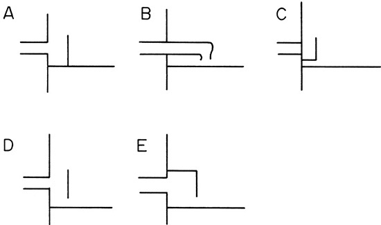
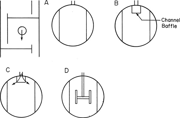
Inlet and outlet ports must be carefully designed to prevent problems (Glitsch, 1985; Kister, 1980a, 1980b, 1990, 1992, 2005; Ludwig, 1997). Inlets should be designed to avoid both excessive weeping and entrainment when a high-velocity stream is added. Several acceptable designs for a feed or reflux to the top tray are shown in Figure 10-8. Baffle plates and pipe elbows prevent high-velocity fluid from shooting across the tray. Designs in Figures 10-8D and 10-8E do not allow excessive entrainment and can be used if there is likely to be vapor in the inlet stream. Intermediate feed introduction is similar, and several common designs are shown in Figure 10-9. Low-velocity liquid feeds can be input through the column side (Figure 10-9A). Higher velocity feeds and feeds containing vapor require baffles as shown in Figures 10-9B and 10-9C. Vapor is directed sideways or downward to prevent excessive entrainment. When feed contains a large quantity of vapor, the feed tray should have extra space for disengagement of liquid and vapor. For large-diameter columns some type of distributor, such as the one shown in Figure 10-9D, is often used.
Vapor returns at the bottom of columns should be at least 12 in. above liquid surge levels. Vapor inlets should be parallel to seal pans and liquid surfaces, as shown in Figure 10-10A. Seal pans keep liquid in downcomers. Vapor inlets should not el-down to impinge on liquid, as shown in Figure 10-10B. When a thermosiphon reboiler (a common type of reboiler) is used, a split drawoff (Figure 10-10C) is useful to retain a liquid head. Since there is usually no pump between the column and the reboiler, driving pressure to move liquid from the column into the reboiler is based on the column’s liquid head. This head must be large enough to overcome pressure drop in the lines and reboiler. For kettle-type reboilers liquid is on the shell side, and shell-side fouling needs to be included in pressure drop calculations. The recommended height from kettle overflow baffles to the column vapor inlet is approximately 2 m (Lieberman and Lieberman, 2008). Smaller clearances can eventually result in flooding because of high liquid levels in the column bottom.
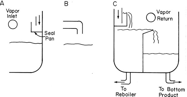
FIGURE 10-10. Bottom vapor inlet and liquid drawoffs; (A) correct—inlet vapor parallel to seal pan, (B) incorrect—inlet vapor el-down onto liquid, (C) bottom drawoff with thermosiphon reboiler
Intermediate liquid drawoffs require some method for disengaging liquid and vapor. An inexpensive way to do this is with a downcomer tapout (Figure 10-11A). A more expensive but surer method is to use a chimney tray (Figure 10-11B). Chimney trays provide enough liquid volume to fill lines and start pumps. There are no holes or valves in the deck of this tray; thus, it does not provide for mass transfer and should not be counted as an equilibrium stage. Chimney trays must often support quite a bit of liquid; therefore, mechanical design is important (Kister, 1990). An alternative to chimney trays is to use a downcomer tapout with an external surge drum.
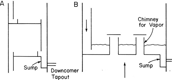
FIGURE 10-11. Intermediate liquid drawoff; (A) downcomer sump, (B) chimney tray (downcomer to next tray not shown)
The design of vapor outlets is relatively easy and is less likely to cause problems than liquid outlets (Kister, 1990). The main consideration is that lines must be large enough to have a modest pressure drop. At the top of the column a demister may be used to prevent liquid entrainment. An alternative is to put a knockout drum in the line before any compressors.
10.2 Tray Efficiencies
Tray efficiencies are introduced in Chapter 4. In this section they are discussed in more detail, and simple methods for estimating efficiency values are explored. The effect of mass transfer rates on stage efficiency is discussed in Chapter 16.
The overall efficiency, EO, is
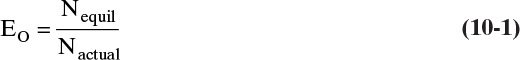
Because partial reboilers and partial condensers have different efficiencies than trays, they should not be included in determination of the number of equilibrium stages required. The overall efficiency is extremely easy to measure and use; thus, it is the most commonly used efficiency value in the plant. However, because it is difficult to relate overall efficiency to fundamental heat and mass transfer processes, it is not generally used in fundamental studies.
The Murphree vapor and liquid efficiencies also are introduced in Chapter 4. The Murphree vapor efficiency is defined as

while the Murphree liquid efficiency is

The physical model used for both of these efficiencies is shown in Figure 10-12. The gas streams and the downcomer liquids are assumed to be perfectly mixed. Murphree also assumed that the liquid on the tray is perfectly mixed, which means x = xout. The term y*out is the vapor mole fraction that would be in equilibrium with the actual liquid mole fraction leaving the tray, xout. In the liquid efficiency, x*out is in equilibrium with the actual leaving vapor mole fraction, yout. The Murphree efficiencies are popular because they are relatively easy to measure, and they are easy to use in calculations (see Figure 4-27B). Unfortunately, there are some difficulties with their definitions. In large columns the liquid on the tray is not well mixed; instead there is a crossflow pattern. If the flow path is long, the more volatile component (MVC) will be preferentially removed as liquid flows across the tray. Thus, in Figure 10-12
xout < x4 < x3 < x2 < x1
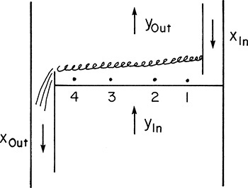
Since xout and hence y*out are based on the lowest liquid concentration on the tray, it is possible to have y*out < yout because yout is an average. The result is EMV > 1, which is often observed in large-diameter columns. Although not absolutely necessary, it is desirable to have efficiencies defined so that they range between 0 and 1. A second and more serious problem with Murphree efficiencies is that in multicomponent systems efficiencies of different components must be different. Fortunately, for binary systems the Murphree efficiencies are the same for both components. In multicomponent systems not only are the efficiencies different, but on some trays they may be negative. This is both disconcerting and extremely difficult to predict. Despite these problems, Murphree efficiencies remain popular. Overall and Murphree vapor efficiencies are related by the following equation, which is derived in Problem 12.C4.
The point efficiency is defined in a fashion very similar to the Murphree efficiency:

where prime indicates that all concentrations are determined at a specific point on the tray. The Murphree efficiency can be determined by integrating all of the point efficiencies (which will vary from location to location) on the tray. Typically, point and Murphree efficiencies are not equal. Although point efficiency is difficult to measure in a commercial column, it can often be predicted from heat and mass transfer calculations. Thus, it is used for prediction and for scale-up.
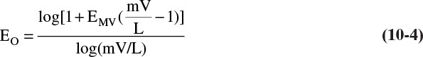
In general, tray efficiency depends on vapor velocity, which is illustrated schematically in Figure 10-13. Trays are designed to give a maximum efficiency at the design condition. At higher vapor velocities, entrainment increases. When entrainment becomes excessive, efficiency plummets. At vapor velocities less than the design rate, mass transfer is less efficient. At very low velocities trays start to weep, and efficiency again plummets. Trays with good turndown characteristics (e.g., valve trays) have a wide maximum, so there is little loss in efficiency when vapor velocity changes.
Best practice is to predict efficiency based on data for the chemical system in the same type of column of the same size for a range of velocities. Fractionation Research Institute (FRI) has reams of efficiency data, but until recently, most data were available to members only, which included most large chemical and oil companies. The second best approach is to have efficiency data for the same chemical system but with a different type of tray. Much older data in the literature are for bubble-cap or sieve trays. Usually, efficiency of valve trays is equal to or better than sieve tray efficiency, which is equal to or better than bubble-cap tray efficiency. Thus, if bubble-cap efficiencies are used for a valve tray column, the design will be conservative. The third best approach is to use efficiency data for a similar chemical system.
If data are not available, a detailed calculation of the efficiency can be made on the basis of fundamental mass and heat transfer calculations. With this method, you first calculate point efficiencies from heat and mass transfer calculations and then determine Murphree and overall efficiencies from flow patterns on the tray. Unfortunately, the results are often not extremely accurate. A simple application of this method is developed in Chapter 16.
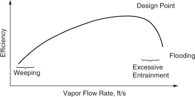
The simplest approach is to use a correlation to estimate efficiency. The most widely used is the O’Connell correlation shown in Figure 10-14 (O’Connell, 1946), which gives an estimate of the overall efficiency as a function of the relative volatility α of the key components times the liquid viscosity µ (in centipoise) at the feed composition. Both α and µ are determined at average column temperature and pressure. Efficiency drops as viscosity increases, since mass transfer rates are lower. Efficiency drops as relative volatility increases, since amount of mass that must be transferred to obtain equilibrium increases. Scatter in the data is evident in Figure 10-14. O’Connell was probably studying bubble-cap columns; thus, the results are conservative for sieve and valve trays (Walas, 1988). Walas surveys a large number of tray efficiencies for a variety of tray types. O’Brien and Schultz (2004) report that many petrochemical towers are designed with stage efficiencies in the 75% to 80% range. Although these columns are probably valve trays, the efficiency range agrees with O’Connell’s correlation. Seider et al. (2009) recommend a first estimate of 70%. Recent FRI data are discussed by Kister (2008), who notes that for low volatility systems, errors in vapor-liquid equilibrium (VLE) data have an enormous effect on measured overall efficiency. Vacuum systems, not included in Figure 10-14, typically have efficiencies of 15% to 20% (O’Brien and Schultz, 2004).
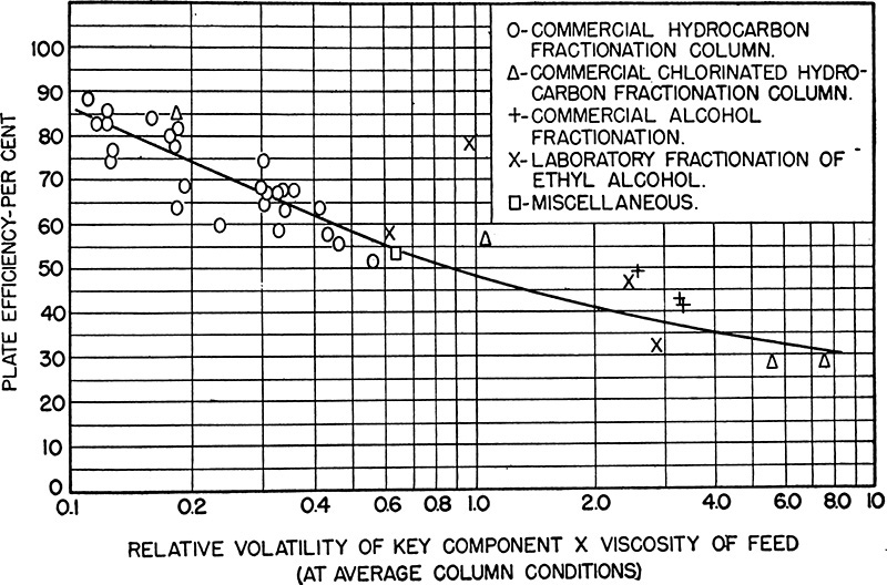
FIGURE 10-14. O’Connell correlation for overall efficiency of distillation columns from O’Connell (1946). Reprinted from Transactions Amer. Inst. Chem. Eng., 42, 741 (1946), copyright 1946, American Institute of Chemical Engineers
For computer and calculator use it is convenient to fit the data points to an equation. When this was done using a nonlinear least-squares routine, the result (Kessler and Wankat, 1988) was
Equation (10-6) is not an exact fit to O’Connell’s curve, since O’Connell apparently used an eyeball fit. Ludwig (1997) discusses other efficiency correlations.
EXAMPLE 10-1. Overall efficiency estimation
A sieve plate distillation column is separating a feed that is 50.0 mol% n-hexane and 50.0 mol% n-heptane. The feed is a saturated liquid. Plate spacing is 24.0 in. Average column pressure is 1.0 atm. Distillate composition is xD = 0.999 (mole fraction n-hexane) and xB = 0.001. The feed rate is 1000.0 lbmol/h. The internal reflux ratio L/V = 0.8. The column has a total reboiler and a total condenser. Estimate the overall efficiency.
Solution
To use the O’Connell correlation we need to estimate α and μ at feed composition and the average temperature and pressure of the column. Column temperature can be estimated from equilibrium (DePriester chart). The following values are generated from Figure 2-12:
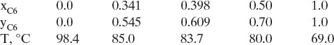
Relative volatility is α = (y/x)/[(1 – y)/(1 – x)]. The average temperature can be estimated several ways:
Arithmetic average T = (98.4 + 69.0)/2.0 = 83.7, α = 2.36
Average at x = 0.5, T = 80.0, α = 2.33
Not much difference. Use α = 2.35 corresponding to approximately 82.5°C.
The liquid viscosity of the feed can be estimated (Reid et al., 1977, p. 462) from
The pure component viscosities can be estimated from
where µ is in cP and T is in Kelvin (Reid et al., 1977, App. A).
nC6: A = 362.79, B = 207.08
nC7: A = 436.73, B = 232.53
These equations give µC6 = 0.186, µC7 = 0.224, and µmix = 0.204. Then αµmix = 0.480. From Eq. (10-6), EO = 0.62, while from Figure 10-14, EO = 0.59. To be conservative, the lower value would probably be used.
Note that once Tavg, αavg, and µfeed have been estimated, calculating EO is straightforward.
Efficiencies can be scaled up from laboratory data taken with an Oldershaw column (a laboratory-scale, sieve tray column) (Fair et al., 1983; Kister, 1990). Overall efficiency measured in Oldershaw columns is often very close to point efficiencies measured in large commercial columns. This similarity is illustrated in Figure 10-15, where vapor velocity has been normalized with respect to fraction of flooding (Fair et al., 1983). Point efficiencies can be converted to Murphree and overall efficiencies once a model for tray flow pattern has been adopted (see Section 16.6). For very complex mixtures, entire distillation designs can be done using Oldershaw columns by changing the number of trays and the reflux rate until a combination that does the job is found. Since commercial columns have an overall efficiency equal to or greater than that of Oldershaw columns, this combination also works in commercial columns. This approach eliminates the need to determine VLE data (which may be quite costly), and it also eliminates the need for complex calculations. Oldershaw columns also allow you to observe foaming problems (Kister, 1990).
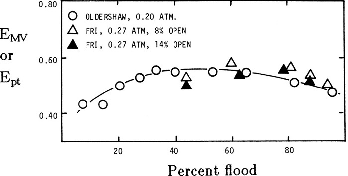
FIGURE 10-15. Overall efficiency of 1.0-in. diameter Oldershaw column compared to point efficiency of 4.0-ft diameter FRI column. System is cyclohexane/n-heptane from Fair et al. (1983). Reprinted with permission from Ind. Eng. Chem. Process Des. Develop., 22, 53 (1983), copyright 1983, American Chemical Society
In many respects the most difficult part of determining design conditions for staged and packed columns is determining physical properties. For hand calculations good sources are Green and Perry (2008), Perry and Green (1997), Poling et al. (2001), Reid et al. (1977), Smith and Srivastra (1986), and Stephan and Hildwein (1987). Commercial simulators have physical property packages to do this grunt work.
10.3 Column Diameter Calculations
To design a sieve tray column we need to calculate a column diameter that prevents flooding, design tray layout, and design downcomers. Several procedures for designing column diameters have been published in the open literature (Fair, 1963, 1984, 1985; Kister, 1992; Ludwig, 1997). In addition, each equipment manufacturer uses its own procedure. We follow Fair’s procedure, since it is widely known and an option in the Aspen Plus simulator (see Chapter 6 Appendix). This procedure first estimates the vapor velocity that will cause flooding due to excessive entrainment and then uses a rule of thumb to determine operating velocity, and from this result it calculates column diameter. Column diameter is very important in cost calculations and has to be estimated even for preliminary designs. Fair’s method is applicable to sieve, valve, and bubble-cap trays. In Sections 10.3 and 10.5 where hand calculations for diameter and tray layout are discussed, we are essentially forced to use English units because many of the graphs and equations that present required empirical data are in English units. Fortunately, commercial simulators allow you to work in a variety of units, and in Lab 10 in this chapter’s appendix, SI units are used.
Flooding velocity based on net area for vapor flow is determined from
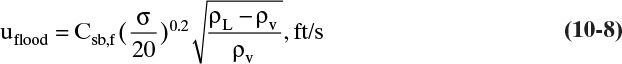
Where σ is surface tension in dynes/cm and Csb,f is a capacity factor. Equation (10-8) is similar to Eq. (2-61), which was used to size vertical flash drums. Csb,f is a function of flow parameter
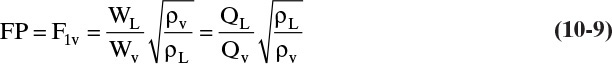
where WL and Wv are mass flow rates of liquid and vapor, QL and QV are volumetric flow rates, and densities are mass densities. The correlation for Csb,f is shown in Figure 10-16 (Fair and Matthews, 1958). For computer use it is convenient to fit the curves in Figure 10-16. Results of a nonlinear least-squares regression analysis (Kessler and Wankat, 1988) for 6.0-in. tray spacing are
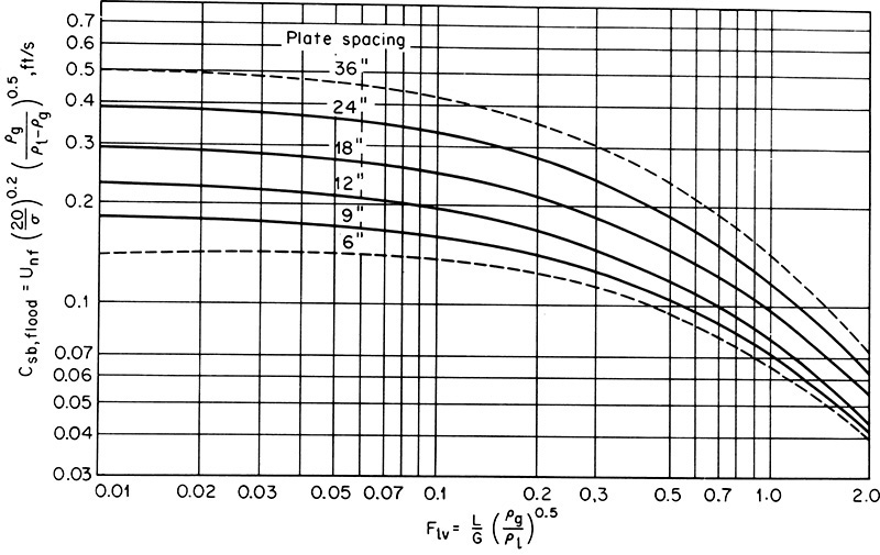
FIGURE 10-16. Capacity factor for flooding of sieve trays from Fair and Matthews (1958). Reprinted with permission from Petroleum Refiner, 37 (4), 153 (1958), copyright 1958, Gulf Pub. Co.
for 12.0-in. tray spacing
for 18.0-in. tray spacing
for 24.0-in. tray spacing
and for 36.0-in. tray spacing
The same flooding correlation but in metric units is available in graphical form (Fair, 1985). Figure 10-16 and Eqs. (10-10) predict conservative values for the flooding velocity.
The flooding correlation assumes that β, the ratio of the area of the holes, Ahole, to the active area of the tray, Aactive, is equal to or greater than 0.1. If β < 0.1, then the flooding velocity calculated from Eq. (10-8) should be multiplied by a correction factor (Fair, 1984). If β = 0.08, the correction factor is 0.9, while if β = 0.06, the correction factor is 0.8. Note that this is a linear correction and can easily be interpolated.
Tray spacing, which is required for the flooding correlation, according to Kister (2008) is usually selected according to maintenance requirements because it has little effect on tray efficiency; however, with the smaller tray spacing there are more trays in the column and more separation can be obtained (Pilling and Summers, 2012). If feeds are very clean and nonfouling, then smaller tray spacing will be advantageous. In refineries and biorefineries where the feeds tend to be both dirty and fouling, a tray spacing that allows routine maintenance is required. Sieve trays are spaced 6 to 36 in. apart with 12 to 16 in. being a common range for smaller towers. In columns less than about 1.2 m in diameter, a tray spacing of 0.45 m is satisfactory because workers can reach through a side entry for maintenance (Torzewski, 2009). For columns from 1.2 to 3.0 m, workers need to be able to crawl through the column, and minimum 0.6 m spacing is required. For columns greater than 3.0 m in diameter, the tray spacing must be greater than 0.6 m because the heavy support beams required to support the trays restrict access (see Figure 10-7). With a typical 24-in. (0.6096 m) tray spacing, Csb,f ∼ 0.33 ft/s (Biegler et al., 1997).
Operating vapor velocity is determined as
where the fraction can range from 0.65 to 0.9. Jones and Mellbom (1982) suggest using a value of 0.75 for the fraction for all cases. Higher fractions of flooding do not greatly affect overall system cost, but they do restrict flexibility. Operating velocity uop can be related to molar vapor flow rate
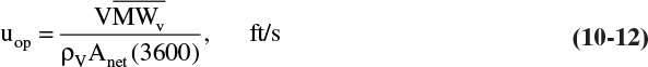
where 3600 converts from hours (in V) to seconds (in uop). Net area for vapor flow is

where η is the fraction of the column cross-sectional area that is available for vapor flow above the tray. Then 1 – η is the fraction of the column area taken up by one downcomer. Typically η lies between 0.85 and 0.95; its value can be determined exactly once tray layout is finalized. Equations (10-12) and (10-13) can be solved for column diameter.
If the ideal gas law holds,

and Eq. (10-14) becomes

Note that these equations are dimensional, since Csb is dimensional.
Since terms in Eqs. (10-8) to (10-16) vary from stage to stage, calculations done at different locations will predict different diameters. Use the largest diameter, and round it off to the next highest half-foot increment. (e.g., a 9.18-ft column is rounded off to 9.5 ft). Ludwig (1997) and Kister (1990) suggest using a minimum column diameter of 2.5 ft; that is, if the calculated diameter is 2.0 ft, use 2.5 ft instead, since it is usually no more expensive. These small columns typically use cartridge trays that are prefabricated outside the column (Ludwig, 1997). Columns with diameters less than 2.5 ft are usually constructed as packed columns. If diameter calculations are done at the top and the bottom of the column and above and below the feed, one of these locations will be very close to the maximum diameter, and design based on the largest calculated diameter will be satisfactory.
For columns operating at or above atmospheric pressure, pressure is essentially constant in the column. If we substitute Eqs. (10-8) and (10-15) in Eq. (10-16), calculate conditions at both the top and the bottom of the column, take the ratio of these two equations, and simplify, the result is

The last two terms on the right-hand side are usually close to 1.0, although when water and organics are separated the surface tension term could be approximately 1.1 (water is the bottom product) or 0.9 (water is the distillate product). The ratio of temperatures is always <1.0 with a range for binary separations typically from 0.9 to 0.99, although it can be lower for distillation at low temperatures. For distillation of homologous series, the molecular weight term is <1, while the liquid density term is probably >1. Since you would not expect large differences, the product of these terms is probably ∼1. For distillation of water and an organic if water is the bottoms product, the molecular weight term is <1, while the density term is >1, and the product of the two terms is probably close to 1. If water is the distillate product, these two terms flip, and the product of the two terms probably remains close to 1. For a saturated vapor feed the vapor velocity term is >1.0 and can range from approximately 1.1 to 2. For a saturated liquid feed this term is very close to 1.0.
As a rule of thumb, if the feed is a saturated liquid and a homologous series is being distilled, the ratio of diameters is probably <1, and the diameter calculated at the bottom is probably larger. This is also true with a saturated liquid feed if the distillation is water from organics and water is the distillate product, but if water is the bottoms product (more common), either the top or the bottom diameter can be larger. If the feed is a saturated vapor, the ratio of the diameters is probably >1, and you should design at the top; however, when water and an organic are distilling with water as the distillate product and for cryogenic distillation, the ratio of diameters could be greater than or less than one.
If there is a very large change in the vapor velocity in the column, the calculated diameters can be quite different. Occasionally, columns are built in two sections of different diameter to take advantage of this situation, but this solution is economical only for large changes in diameter. If a column with a single diameter is constructed, the efficiencies in different parts of the column may vary considerably (see Figure 10-13). This variation in efficiency has to be included in the design calculations. Another alternative is to attempt to balance the required diameters by adjusting vapor velocities. This method is discussed in Section 10.4.
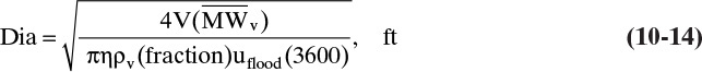
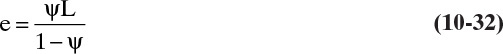
The design procedure sizes the column to prevent flooding caused by excessive entrainment. Flooding can also occur in the downcomers, and this case is discussed later. Excessive entrainment can also cause a large drop in stage efficiency because liquid that has not been separated is mixed with vapor. The effect of entrainment on the Murphree vapor efficiency can be estimated from

where EMV is the Murphree efficiency without entrainment, and ψ is the fractional entrainment defined as

where e is the mol/h of entrained liquid. The relative entrainment ψ for sieve trays can be estimated from Figure 10-17 (Fair, 1963). Once the corrected value of EMV is known, the overall efficiency can be determined from Eq. (10-7). Usually, entrainment is not a problem until fractional entrainment is >0.1, which occurs when operation is in the range of 85% to 100% of flood (Ludwig, 1997). Thus, a 75% of flood value should have a negligible correction for entrainment. This can be checked during the design procedure (see Example 10-3).
FIGURE 10-17. Entrainment correlation from Fair (1963). Reprinted with permission from Smith, B. D., Design of Equilibrium Stage Processes, copyright 1963, McGraw-Hill, New York
EXAMPLE 10-2. Diameter calculation for tray column
Determine the required diameter at the column top for the distillation column in Example 10-1.
Solution
We can use Eq. (10-16) with 75% of flooding. Since distillate is almost pure n-hexane, we can approximate properties as pure n-hexane at 69.0°C.
Physical properties: ρL = 0.659 g/ml (at 20°); viscosity = 0.22 cP; MW = 86.17 (Perry and Green, 1984). Surface tension σ = 13.2 dynes/cm (Reid et al., 1977, p. 610). The ideal gas law is used to estimate vapor density.
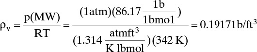
ρL = (0.659)(62.4) = 41.12 lb/ft3 (will vary but not a lot). At the top of the column MWL = MWv and
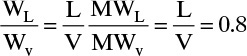
The flow parameter is
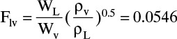
Ordinate from Figure 10-16 for 24-in. tray spacing, Csb = 0.36 while Csb = 0.38 from Eq. (10-10e). Then
K = 0.35 if Eq. (10-10e) is used. The lower value is used for a conservative design. From Eq. (10-8)
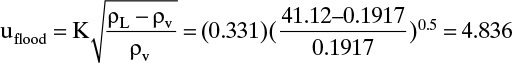
We will estimate η as 0.90. V = L + D. From external mass balances, D = 500.0. Since L = V(L/V) and L/V + 0.8,
Diameter Eq. (10-16) becomes
Since Fair’s diameter calculation procedure is conservative, an 11.0-ft diameter column would probably be used. If η = 0.95, Dia = 10.74 ft; thus, the value of η is not critical. This is a large-diameter column for this feed rate. The reflux rate is quite high, and thus, V is high, which leads to a larger diameter. The effect of location on the diameter calculation can be explored by doing Problem 10.D2. Since Problem 10.D2 predicts a 12.0-ft diameter, design the column at the bottom. This result agrees with the rule of thumb given after Eq. (10-17) (hexane and heptane are part of the homologous series of alkanes). The value of η = 0.9 is checked in Example 10-3. Column pressure effects are explored in Problem 10.C1.
10.4 Balancing Calculated Diameters
Occasionally calculated diameters at different column locations will vary by a large factor. For example, for distillation of a vapor feed of ethanol and water, calculated diameter at the top of the column was 3.7 times as large as the calculated diameter at the bottom of the column (Wankat, 2007a). For distillation of a liquid feed of acetic acid and water (water is more volatile), calculated diameter at the bottom was 1.7 times the calculated diameter at the top (Wankat, 2007b).
Instead of building the entire column at the larger diameter, it may be possible to balance column diameters. Equation (10-14) shows that column diameter is directly proportional to the square root of vapor velocity. If we can reduce V at the location with the largest calculated diameter and increase V elsewhere, we may be able to decrease column diameter significantly with very little effect on purity.
For a vapor feed, column diameter is often largest in the enriching section. We can reduce diameter by reducing V by condensing all or part of the feed or by condensing vapor inside the column with an intermediate condenser (Jones and Wilson, 1996). Three methods for doing this are shown in Figure 10-18. In all cases, there will be a reduction in purity if L/D and N are constant. (Why?) Often, adding a few stages or slightly increasing reflux ratio will restore purity to the desired value. If calculated diameters are markedly different, then the net column volume and column cost will probably be reduced despite the use of more stages. For ethanol-water distillation with a vapor feed, a reduction in column volume of 58% was achieved with a two-enthalpy feed (Figure 10-18B) and of 42% with an intermediate condenser with constant heating and cooling loads. Cooling the entire feed (Figure 10-18A) could reduce volume significantly, but |Qc| and QR have to be increased (Wankat, 2007a). Total annual costs (TAC), Eq. (11-22), were not significantly different for the vapor feed and two-enthalpy feed columns, except when refrigeration was required, the two-enthalpy feed system often had significantly lower TAC (Wankat, 2015).
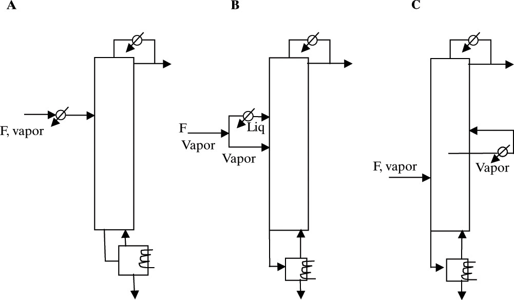
FIGURE 10-18. Column balancing methods for vapor feed with largest calculated diameter at the top. (A) Cool entire feed. (B) Use two-enthalpy feed and cool portion of feed. (C) Intermediate condenser
For a liquid feed system with the largest calculated diameter at the column bottom, we want to reduce V at the column bottom and increase V higher up the column. Reboiler duty can be reduced (V decreases) if we heat the entire feed (Figure 10-19A), use a two-enthalpy feed vaporizing a portion of feed (Figure 10-19C), or use an intermediate reboiler (Figure 4-23A). If the number of stages and the reflux ratio are constant, these methods will all result in lower purity. Again, adding a few stages often solves this difficulty. For acetic acid–water distillation with constant total heat loads, a reduction of column volume of 54% was obtained with an intermediate reboiler (Figure 4-23A), vapor bypass (Figure 10-19C) reduction was 9.6%, two-enthalpy feed (Figure 10-19B) reduction was 12%, and entire feed heating (Figure 10-19A) reduction was 10% (Wankat, 2007b).
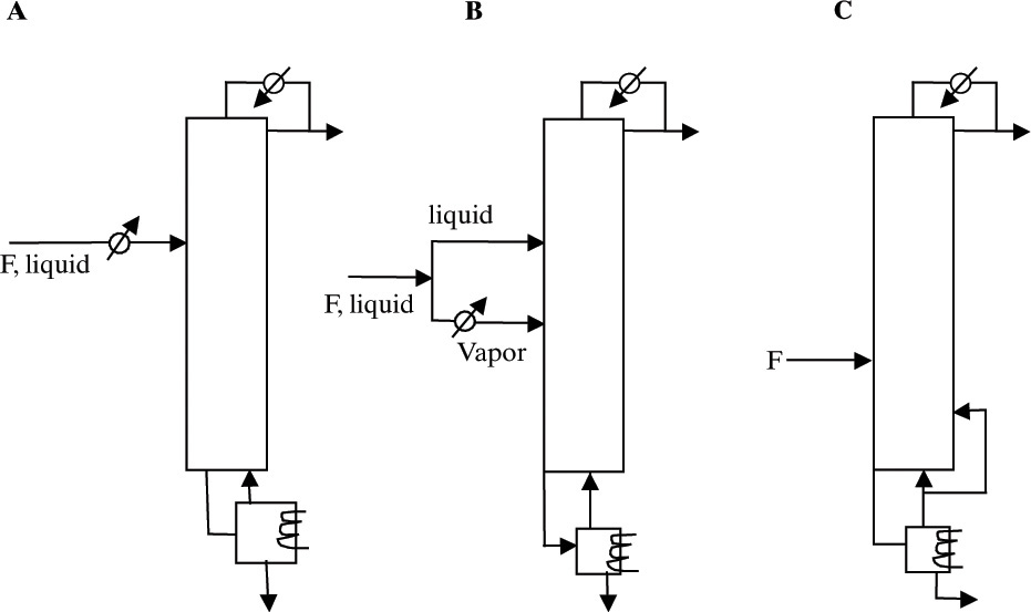
FIGURE 10-19. Column balancing methods for liquid feed with largest calculated diameter at the bottom. (A) Heat entire feed. (B) Use two-enthalpy feed and heat portion of feed. (C) Vapor bypass
The addition of heat exchangers and an additional feed stage (Figures 10-18A, 10-18B, 10-19A, and 10-19B) are straightforward and should cause no operating problems. Intermediate condensers and reboilers (Figures 10-18C and 4-23A) are commonly used (Jones and Wilson, 1996); however, they can make startup significantly more difficult (Sloley, 1996). The best system can be determined with computer simulations (see Problem 10.G1) coupled with economics (see Chapter 11).
10.5 Sieve Tray Layout and Tray Hydraulics
Tray layout is an art with its own rules. This section follows the presentations of Ludwig (1997), Bolles (1963), Fair (1963, 1984, 1985), Kister (1990, 1992, 2008), and Lockett (1986), and more details are available in those sources. Holes in a sieve plate are not scattered randomly. Instead, a detailed pattern is used to ensure even flow of vapor and liquid on the tray. Punched holes in the tray usually range in diameter, do, from 1/8 to 1.0 in. In the range from 1/2 to 1.0 in., efficiency is constant and at its highest level. In vacuum operation 1/8-in. holes with the holes punched upward are often used to reduce entrainment and minimize pressure drop. In normal operation holes are punched downward, since this is much safer for maintenance personnel. In fouling applications, holes are 1/2 in. or larger. For clean service, 1/2 in. is a reasonable first guess for hole diameter.
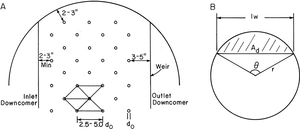
Equilateral triangular pitch shown in Figure 10-20A is a common tray layout. Use of standard punching patterns is cheaper than use of a nonstandard pattern. Holes are spaced from 2.5 do to 5.0 do apart, with 3.8 do a reasonable average. The region containing holes should have a minimum 2- to 3-in. clearance from the column shell and downcomer inlet. To allow for disengagement of liquid and vapor a 3- to 5-in. minimum clearance is used before the downcomer weir. Since flow on the trays is very turbulent, vapor does not go straight up from the holes. The active hole area is considered to be 2 to 3 in. from the peripheral holes; thus, the area up to the column shell is active. The fraction of the column that is taken up by holes depends on hole size, pitch, hole spacing, clearances, and downcomer sizes. Typically, 4% to 15% of the entire tower area is hole area, which corresponds to a value of β = Ahole/Aactive of 6% to 25%. The average value of β is between 7% and 16%, with 10% a reasonable first guess.
The β value is selected so that vapor velocity through the holes, vo, lies between the weep point and the maximum velocity. The exact design point should be selected to give maximum flexibility in operation. Thus, if a reduction in feed rate is much more likely than an increase in feed rate, the design vapor velocity will be close to the maximum. Vapor velocity through the holes, vo, in feet per second (ft/s) can be calculated from
where V is lbmol/h of vapor, ρv is vapor density in lb/ft3, and Ahole is total hole area on the tray in ft2. Obviously, Ahole can be determined from tray layout.

The active area can be estimated as
Downcomer geometry is shown in Figure 10-20B. From this and geometric relationships, downcomer area Ad can be determined from
where θ is in radians. Combining Eqs. (10-20d), (10-22a), and (10-22b), we can solve for angle θ and weir length (Table 10-1). Typically, the ratio of lweir/Dia ranges from 0.6 to 0.75.

If liquid is unable to flow down downcomers fast enough, the liquid level will increase, and if it keeps increasing until it reaches the weir top of the tray above, the tower will flood. This occurrence is downcomer flooding. Downcomers are designed based on pressure drop and liquid residence time, and their cost is relatively small. Thus, downcomer design is done only during final equipment sizing.
A tray and downcomer are drawn schematically in Figure 10-21, which shows pressure heads caused by various hydrodynamic effects. The head of clear liquid in the downcomer, hdc, can be determined from the sum of heads that must be overcome.

The head of liquid required to overcome the pressure drop of gas on a dry tray, hΔp,dry, can be measured experimentally or estimated (Ludwig, 1995) from

where vo is the vapor velocity through holes in ft/s from Eq. (10-19), and hΔp,dry is in inches. Orifice coefficient, Co, can be determined from the correlation of Hughmark and O’Connell (1957), which can be fit by the following equation (Kessler and Wankat, 1988):

where ttray is tray thickness. The minimum value for do/ttray is 1.0.
Weir height, hweir, is the actual height of the weir. Minimum weir height is 0.5 in. with 2 to 4 in. more common. The weir must be high enough that the opposite downcomer remains sealed and always retains liquid. The height of the liquid crest over the weir, hcrest, can be calculated from the Francis weir equation.
where hcrest is in inches. In this equation, Lg is the liquid flow rate in gal/min that is due to both L and entrainment, e, determined from Figure 10-17. lweir is the length of the straight weir in feet. The factor Fweir (Figure 10-22) takes into account curvature of the column wall in the downcomer (Bolles, 1946, 1963; Ludwig, 1997). An equation for this figure is available (Bolles, 1963). For large columns where lweir is large, Fweir approaches 1.0.
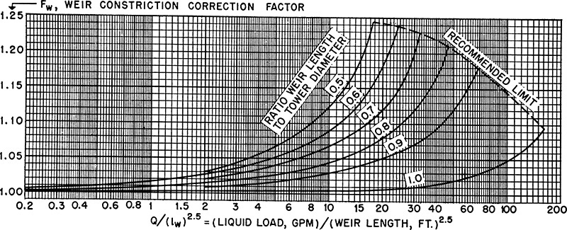
FIGURE 10-22. Weir correction factor, Fweir, for segmental weirs from Bolles (1946). Reprinted with permission of Petroleum Processing
On sieve trays, the liquid gradient, hgrad, across the tray is often very small and is usually ignored. There is a frictional loss due to flow in and under the downcomer onto the tray, hdu, that can be estimated from the empirical equation (Ludwig, 1997; Bolles, 1963).

where hdu is in inches, and Adu is the flow area under the downcomer apron in ft2. The downcomer apron typically has a 1-in. gap above the tray.
The value of hdc calculated from Eq. (10-23) is the head of clear liquid in inches. In an operating distillation column, liquid in the downcomer is aerated and has a lower density than clear liquid; thus, the height of aerated liquid in the downcomer is greater than hdc. Height of the aerated liquid in the downcomer, hdc,aerated, can be estimated (Fair, 1984) from
where ϕdc is relative froth density. In normal operation, ϕdc = 0.5 is satisfactory, while 0.2 to 0.3 should be used in difficult cases (Fair, 1984). To avoid downcomer flooding, tray spacing must be greater than hdc,aerated. Thus, in normal operation the tray spacing must be greater than 2.0 hdc.
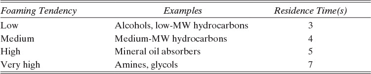
Downcomers are designed for a liquid residence time of 3 to 7 s. Minimum residence times are listed in Table 10-2 (Kister, 1980e, 1990; Ludwig, 1997). Residence time in a straight segmental downcomer (in seconds) is

where the 3600 converts hours to seconds (from L + e) and the 12 converts hdc in inches to feet. Density ρL is the density of clear liquid, and hdc is the height of clear liquid. Equation (10-30) is used to make sure there is enough time to disengage liquid and vapor in downcomers. With saturated liquid feeds downcomers are designed for the stripping section where the liquid flow rate is largest.
Figure 10-13 shows that the two limits to acceptable tray operation are excessive entrainment and excessive weeping. Although weep and dump points are difficult to determine exactly, an approximate analysis can be used to ensure operation is above the weep point. Liquid will not drain through holes as long as the sum of heads due to surface tension, hσ, and gas flow, hΔp,dry, are greater than a function depending on liquid head. This condition for avoiding excessive weeping can be determined from Fair’s (1963) graphical correlation or estimated (Kessler and Wankat, 1988) as
where x = hweir + hcrest + hgrad. Equation (10-31a) is valid for β ranging from 0.06 to 0.14 and is conservative. Dry tray pressure drop is determined from Eqs. (10-24) and (10-25). Surface tension head hσ can be estimated (Fair, 1963) from
where σ is in dynes/cm, ρL in lb/ft3, do in inches, and hσ in inches of liquid.
EXAMPLE 10-3. Tray layout and hydraulics
Determine the tray layout and pressure drops for the distillation column in Examples 10-1 and 10-2. Determine if entrainment or weeping is a problem and if the downcomers will work properly. Do these calculations only at the top of the column.
Solution
This is a straightforward application of the equations in this section. We can start by determining entrainment. In Example 10-2 we obtained Flv = 0.0546. Figure 10-17 at 75% of flooding gives ψ = 0.045. Solving for e,
Since L = (L/V)V = 2000.0 lbmol/h,
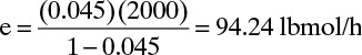
and L + e = 2094.24 lbmol/h. This amount of entrainment is quite reasonable.
The geometry calculations proceed as follows for an 11.0-ft diameter column:
Atotal = π(Dia)2/4 = (π)(11.0)2/4 = 95.03 ft2
Eq. (10-22b), Ad = (1 – 0.9)(95.03) = 9.50 ft2
Table 10-1 gives lweir/Dia = 0.726 or lweir = 8.0 ft
Eq. (10-21b), Aactive = (95.03)(1 – 0.2) = 76 ft2
Eq. (10-20b), Ahole = (0.1)(76.0) = 7.6 ft2
We will use 14-gauge standard tray material (ttray = 0.078 in.) with 3/16-in. holes. Thus, do/ttray = 2.4.
From Eq. (10-19)
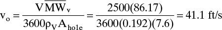
where ρv is from Example 10-2. This hole velocity is reasonable.
The individual pressure drop terms can now be calculated. The orifice coefficient Co is from Eq. (10-25):
Co = 0.85032 – 0.04231(2.4) + 0.0017954(2.4)2 = 0.759
From Eq. (10-24):

In this equation ρwater at 69°C was found from Perry and Green (1984, p. 3–75).
A weir height of hweir = 2 in. will be selected. Correlation factor Fweir can be found from Figure 10-22. The liquid load in gallons per minute in the abscissa is the liquid flow rate including entrainment, Lg, in gallons per minute.
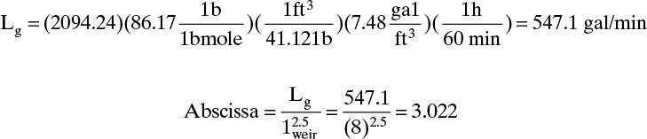
Parameter 1weir/Dia = 0.727. Then Fweir = 1.025. From Eq. (10-26),
We will assume hgrad = 0. The area under the downcomer is determined with a 1.0-in. gap.
From Eq. (10-28), Adu = (1/12)(8) = 2/3 ft2.
From Eq. (10-27),
Total head (total pressure drop across the tray) from Eq. (10-23),
hdc = 2.472 + 2 + 1.577 + 0 + 1.871 = 7.92
This is inches of clear liquid of density 41.12 lbm/ft3. Liquid head can be converted to a pressure drop with two different methods. First,

which is 1.30 kPa. We can also convert the inches of clear liquid of density 41.12 lbm/ft3 to cm Hg. Since the density of mercury is 845.3 lbm/ft3, we have
(7.92 in.)(41.12/845.3)(2.54 cm/in.) = 0.9786 cm Hg = 1.30 kPa.
Since the typical pressure drop for sieve or valve trays is in the range from 0.7 to 1.4 kPa per tray (Woods, 2007), this pressure drop is reasonable.
For the aerated system, ![]() .
.
This value is much less than the 24.0-in. tray spacing, and there should be no problem. The residence time is, from Eq. (10-30),
This is greater than the minimum residence time of 3.0 s.
Weeping can be checked. From Eq. (10-31b),
Then the left-hand side of Eq. (10-31a) is
hΔp,dry + hσ = 2.472 + 0.068 = 2.54
The function x = 2 + 1.577 + 0 = 3.577, and the right-hand side of Eq. (10-31a) is 0.725. The inequality is obviously satisfied. Weeping should not be a problem.
Note that the design should be checked at other locations in the column. Since Problem 10.D2 calculated that a 12-ft diameter is needed in the stripping section, calculations need to be repeated for the stripping section (see Problem 10.D3). Problem 10.D3 shows that backup of liquid in the downcomers might be a problem in the bottom of the column even with a 12-ft diameter. This occurs because ![]() , which is significantly greater than the liquid flow in the top of the column. This problem can be handled by an increase in the gap between the downcomer and the tray.
, which is significantly greater than the liquid flow in the top of the column. This problem can be handled by an increase in the gap between the downcomer and the tray.
Note: Computer simulation programs do these calculations—see Lab 10 in this chapter’s appendix.
10.6 Valve Tray Design
Valve trays, which are illustrated in Figure 10-1, are proprietary devices, and the final design is normally done by the supplier. However, suppliers do not perform optimization studies without receiving compensation for the additional work. In addition, it is always a good idea to know as much as possible about the equipment before making a major purchase. Thus, Bolles’s (1976) nonproprietary valve tray design procedure is very useful. Bolles’s design procedure uses sieve tray design procedures as a basis and modifies it as necessary. One major difference between valve and sieve trays is their pressure drop characteristics. The dry tray pressure drop in a valve tray is shown in Figure 10-23 (Bolles, 1976). As gas velocity increases, Δp first increases and then levels off at a plateau level before increasing again. At first all valves are closed. At the closed balance point, valves start to open. Additional valves open in the plateau region until all valves are open at the open balance point. The head loss in inches of liquid for both closed and open valves can be expressed in terms of the kinetic energy.

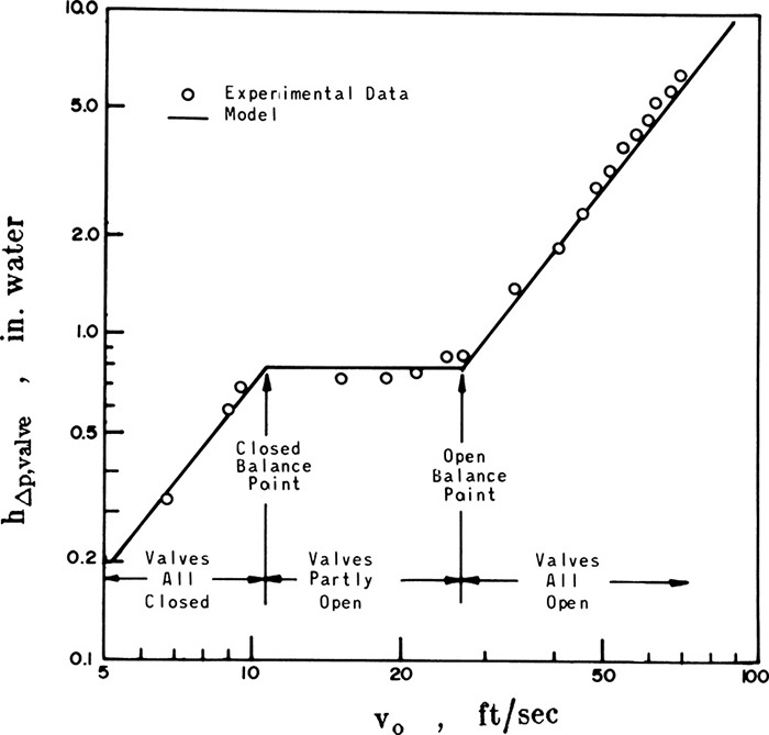
FIGURE 10-23. Dry tray pressure drop for valve tray from Bolles (1976). Reprinted from Chemical Engineering Progress, Sept. 1976, copyright 1976, American Institute of Chemical Engineers
where vo is the velocity of vapor through the holes in the deck in ft/s, g = 32.2 ft/s2, and Kv is different for closed and open valves. For the data shown in Figure 10-23,
Note that hΔp,valve has the same dependence on (v2oρv/ρL) as hΔp,dry for sieve trays in Eq. (10-24).
The closed balance point can be determined by noting that the pressure must support the weight of the valve, Wvalve, in pounds. Pressure is Wvalve/Av, where Av is the valve area in square feet. The pressure drops in terms of feet of liquid density ρL is then

where valve coefficient Cv is introduced to include turbulence losses. For the data in Figure 10-23, Cv = 1.25. Setting Eqs. (10-33) and (10-35) equal allows solution for both closed and open balance points.
where vo,bal is the closed balance point velocity if Kv,closed is used. The values of Kv,closed, Kv,open, and Cv depend on deck thickness and, to a small extent, on valve type (Bolles, 1976).
Most remaining preliminary design steps for columns equipped with valve trays are the same or slightly modified from sieve tray design (Kister, 1990, 1992; Larson and Kister, 1997; Lockett, 1986). Flooding and diameter calculations are the same except the correction factor for Ahole/Aa < 0.1 is replaced by a correction factor for Aslot/Aa < 0.1. The same values for the correction factors are used. Slot area Aslot is the vertical area between tray deck and valve top through which the vapor passes in a horizontal direction. Between balance points slot area is variable and can be determined from the fraction of valves that are open. Pressure drop Eq. (10-23) is the same, while Eq. (10-24) for hΔp,dry is replaced by Eq. (10-34a) or (10-35). Equations (10-26) to (10-30) are unchanged. The gradient across the valve tray, hgrad, is probably larger than on a sieve tray but is often ignored. Valve trays usually operate with higher weirs, and hweir = 3 in. is normal. There are typically 12 to 16 valves per ft2 of active area (Kister, 1990).
Efficiencies of valve trays depend on vapor velocity, valve design, and chemical system being distilled. Except at vapor flow rates near flooding, efficiencies of valve trays are equal to or higher than sieve tray efficiencies, which are equal to or higher than bubble-cap tray efficiencies. Thus, use of the efficiency correlations discussed earlier will result in a conservative design.
10.7 Introduction to Packed Column Design
Instead of staged columns we often use packed columns for distillation, absorption, stripping, and occasionally extraction. Packed columns are definitely more economical for columns less than 2.5 ft in diameter because it is expensive to build a staged column that operates properly in small diameters. In larger packed columns the liquid may tend to channel, and without careful design randomly packed towers may not operate very well; in many cases large-diameter staged columns are cheaper. Packed towers have the advantage of a smaller pressure drop and are therefore commonly used in vacuum fractionation.
In designing a packed tower, packing is chosen based on economic considerations. A wide variety of packings including random and structured are available. Once the packing has been chosen the column diameter and the height of packing are calculated. Column diameter is sized on the basis of either approach to flooding or acceptable pressure drop. Packing height can be found either from an equilibrium stage analysis or from mass transfer considerations. Equilibrium stage analysis is considered here; mass transfer design methods are discussed in Chapter 16.
10.8 Packings and Packed Column Internals
In a packed column used for vapor-liquid contact, the liquid flows over the surface of the packing, and the vapor flows in the void space inside the packing and between pieces of packing. The purpose of the packing is to provide for intimate contact between vapor and liquid with a very large surface area for mass transfer, which according to Eq. (1-4) increases the rate of mass transfer. At the same time, the packing should provide for easy liquid drainage and have a low pressure drop for gas flow. Since packings are often randomly dumped into the column, they also have to be designed so that one piece of packing will not cover up and mask the surface area of another piece.
Packings are available in a large variety of styles, some of which are shown in Figure 10-24. The simpler styles such as Raschig rings are usually cheaper on a volumetric basis but will often be more expensive on a performance basis. Individual rings and saddles are dumped into the column and distributed in a random fashion. Structured or arranged packings (e.g., Glitsch grid, Goodloe, and Koch Sulzer) are carefully placed in the column. Structured packings usually have lower pressure drops and may be more efficient than dumped packings but are often more expensive. Since pressure drop is critical for vacuum columns, structured packings are usually the best choice (Olujic, 2014). Because packings are available in a variety of materials including plastics, metals, ceramics, and glass, they can be used in extremely corrosive service.
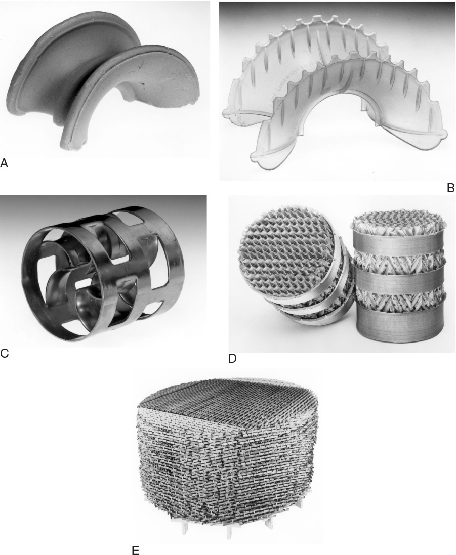
FIGURE 10-24. Types of column packing; (A) ceramic Intalox saddle, (B) plastic super Intalox saddle, (C) Pall ring, (D) GEMPAK cartridge, (E) Glitsch EF-25A grid. Figures A, B, and C courtesy of Norton Chemical Process Products, Akron, Ohio. Figures D and E courtesy of Glitsch, Inc., Dallas, Texas
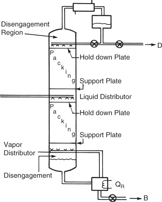
Packing must be properly held in the column to fully utilize its separating power. A schematic diagram of a packed distillation column is shown in Figure 10-25. In addition to the packed sections where separation occurs, sections are needed for distribution of the reflux, feed, and boilup and for disengagement between liquid and vapor. Liquid distributors are critical for proper operation of the column. Small random and structured packings need better liquid and vapor distribution (Kister, 1990, 2005). If (column diameter)/(packing diameter) > ∼40, maldistribution of liquid and vapor is more probable. Maldistribution also reduces the turndown capability of the packing and causes a large increase in HETP at low liquid rates. Liquid maldistribution is explored in Problem 10.D10.
Liquid distributors typically have a manifold with a number of drip points. Bonilla (1993) gives specific recommendations on the number of drip points per square foot. He recommends 6 (10 for high purity) for large packings (random packings ≥2.5 in. or structured packings with crimps >1/2 in.). For small packings (random packings ≤1 in. or structured packings with crimps ≥1/4 in.) he recommends 8 (12 for high purity) at high liquid loads and 10 (14 for high purity) at low liquid loads. Requirements for medium-size packings are between the small and large recommendations. Low liquid loads need more drip points because the liquid tends to spread less. Scale-up of distributors is done by keeping the number of drip points per square foot constant. Redistribution systems may be required on large columns.
Packing is supported by a support plate, which may be a grid or series of bars. A hold-down plate is often employed to prevent packing movement when surges in gas rate occur. Since liquid and vapor are flowing countercurrently throughout the column, there are no downcomers. Additional details on packed tower internals are given by Fair (1985), Green and Perry (2008), Kister (1990, 2005), Ludwig (1997), Strigle (1994), and manufacturers’ literature. Internals of packed columns for absorption or stripping are similar to the distillation column shown in Figure 10-23 but without center feed, reboiler, or condenser.
10.9 Height of Packing: HETP Method
Even though a packed tower has continuous instead of discontinuous contact of liquid and vapor, Peters (1922) realized that it can be analyzed similarly to a staged tower. We assume that the packed portion of the column can be divided into a number of segments of equal height. Each segment acts as an equilibrium stage, and liquid and vapor leaving the segment are in equilibrium. It is important to note that this staged model is not an accurate picture of what is happening physically in the column, but the model can be used for design.
Calculate the number of stages from any staged analysis and then calculate the height as
The HETP, which is measured experimentally, is the height of the packing needed to obtain the change in composition obtained with one theoretical equilibrium contact. HETPs can vary from 1/2 in. (very low gas flow rates in self-wetting packings) to several feet (large Raschig rings). In normal industrial equipment the HETP varies between 1 and 4 ft. The smaller the HETP, the shorter the column and the more efficient the packing.
A common method to measure the HETP is to measure the top and bottom compositions at total reflux and then calculate the number of equilibrium stages. Then

A partial reboiler is usually used but should not be included in the calculation of HETP.
The HETP determined at total reflux is then used at the actual reflux ratio. Ellis and Brooks (1971) found that HETP increases, but the increase is usually quite small until L/D approaches 1.0. Thus, the usual measurement procedure can be used for most design situations.
HETP varies with the packing type and size, chemicals being separated, and gas flow rate. Typical HETP curves are shown in Figure 10-26. The HETP values for several types of packing are listed in the manufacturers’ bulletins and have been compared by Ellis and Brooks (1971), Kister and Larson (1997), Kister et al. (1994), Ludwig (1997), and Walas (1988). Mass transfer results are compared by Furter and Newstead (1973), Green and Perry (2008), Ludwig (1997), and Strigle (1994). Correlations to determine HETP values were developed by Murch (1953) and Whitt (1959), but these do not include modern packings (see Ludwig, 1995). An improved mass transfer model for packings and HETP data for a variety of packings is presented by Bolles and Fair (1982) and is discussed in Chapter 16. The HETPs are different for different chemical systems and higher for larger-size packing. Most packings of the same size have approximately the same HETP. Note from Figure 10-26 that the HETP for a given system and the packing size are roughly constant over a wide range of gas flow rates. This constant value in the usual design range makes the design procedure convenient. As flooding is approached, the efficiency of the contact decreases, and the HETP increases. Also, at very low gas flow rates, the HETP often increases. This occurs because the packing is not completely wet. For self-wetting packings, where capillary action keeps the packing wet, the HETP usually drops at very low gas flow rates.
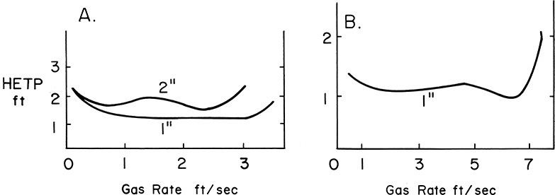
FIGURE 10-26. HETP vs. vapor rate for metal Pall rings; (A) Iso-Octane-Toluene, (B) acetone water. Reprinted with permission from “Pall Rings in Mass Transfer Operations,” 1968 courtesy of Norton Chemical Process Products, Akron, Ohio
HETP values are most accurate if determined from data. If no data are available, generalized mass transfer correlations are used (see Chapter 16). If no information is available, Ludwig (1997) suggests using an average of 1.5 to 2 ft for dumped packings. If the column diameter is greater than 1.0 ft, an HETP greater than 1.0 ft should be used. Another approximate approach is to set HETP equal to column diameter (Ludwig, 1997). Eckert (1979) notes that HETP values for 1-, 1½-, and 2-in. Pall rings are 1, 1½, and 2 ft, respectively. Woods (2007) gives ranges of 0.4 to 0.8 m and 0.7 to 0.9 m for 1.0- and 2-in. Pall rings, respectively. These HETP values are almost independent of the system distilled. A number of other shortcut HETP relationships are summarized by Wang et al. (2005).
Approximate values of HETP for structured packings can be obtained from the following approximate equation (Geankoplis, 2003; Kister, 1992):
where HETP is in meters and ap, the surface area per volume, is in m2/m3. This result is restricted to low-viscosity fluids at moderate or low pressures. Typical HETP values for structured packings range from 0.3 to 0.6 m. Systems with high surface tensions will have higher HETP values. For example, for systems (amines, glycols) with σ ∼ 40 dynes/cm, multiply HETP from Eq. (10-37c) by 1.5, and for aqueous systems with σ ∼ 70 dynes/cm, multiply HETP from Eq. (10-37c) by 2.0 (Anon., 2005). If liquid distribution is not excellent, a 30% to 50% safety factor is suggested.
Since the HETP is often almost constant throughout the usual design range for gas flow rates, concentrations, and reflux ratios, a single HETP value can usually be used in comparing many different designs. This greatly facilitates design. However, HETP can vary significantly within the column because of changes in composition; it can then be estimated for each stage from the mass transfer coefficient (see Sherwood et al., 1975, pp. 521–523 for an example). Alternatively, a mass transfer design approach can be used and is preferred (see Chapter 16).
10.10 Packed Column Flooding and Diameter Calculation
Columns are sized to operate from 65% to 90% of flooding or to have a given pressure drop per foot of packing. Flooding can be more easily measured in a packed column than in a plate column and is usually signaled by a break in the curve of pressure drop versus gas flow rate.
The generalized flooding correlation developed by Sherwood et al. (1938) as modified by Eckert (1970, 1979) is shown in Figure 10-27. Note that the ordinate of Figure 10-27 has units, and these units need to be used in calculations: µ is liquid viscosity in cp, ψ = ρwater/ρL, gc = 32.2 (ft·lbm)/(lbf·s2), densities are lbm/ft3, Δp is inches water/ft, G´ is flux in lb/s-ft2, and L and G are lbm/s. A graph of the same data with an arithmetic scale for the ordinate is available (Geankoplis, 2003; Strigle, 1994), and a graph updated with new data is available (Kister et al., 2007). Packing factor, F, depends on the type and size of the packing. Higher F values have larger pressure drops per foot of packing. F values for dumped packing are in Table 10-3 (Eckert, 1970, 1979; Ludwig, 1997), and F values for structured packings are in Table 10-4 (Fair, 1985; Geankoplis, 2003). As packing sizes increase, F values decrease, and pressure drop per foot decreases. More extensive lists of F values are available in Perry’s Handbook (Perry and Green, 1997) and in Strigle (1994). The effect of packing size on the packing factor can be fit reasonably well with the equation (Bennett, 2000)
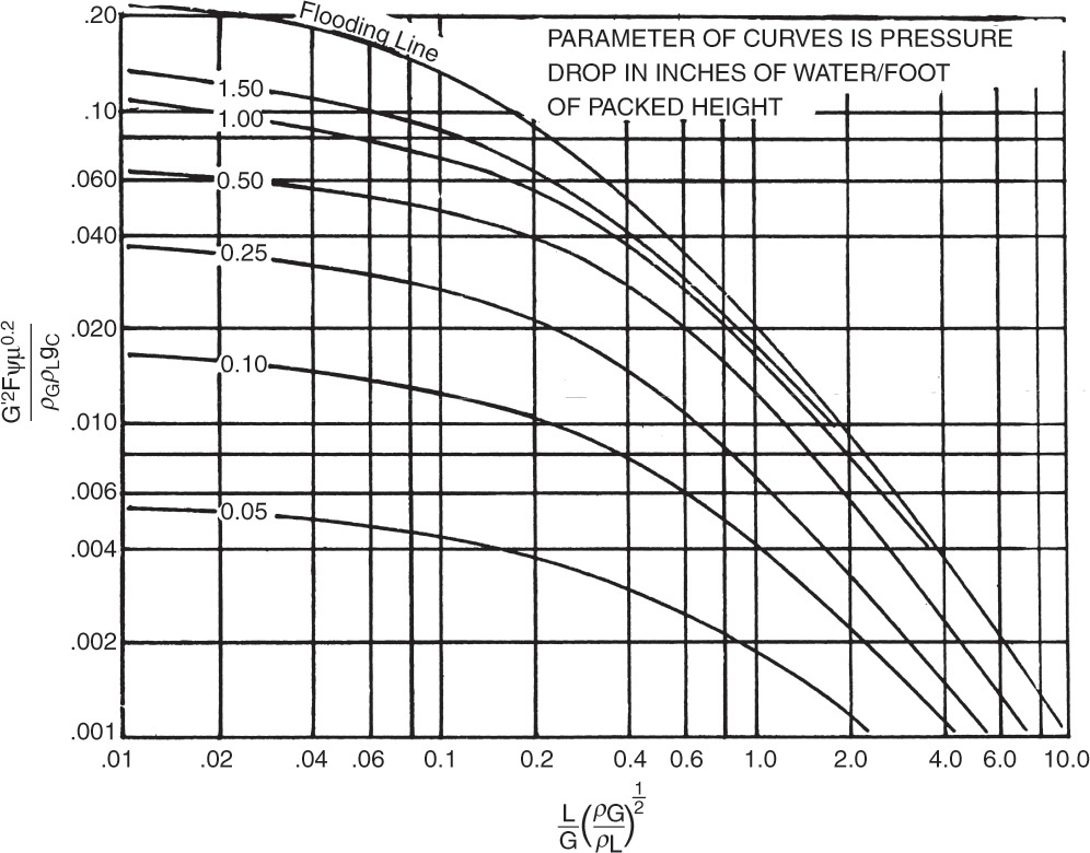
FIGURE 10-27. Generalized flooding and pressure drop correlation for packed columns. Reprinted with permission from Eckert, Chem. Eng. Prog., 66 (3), 39 (1970), copyright 1970 AIChE. Reproduced by permission of the American Institute of Chemical Engineers


Source: Eckert (1970), Ludwig (1997), Coker (1991), Geankoplis (2003)
TABLE 10-3. Parameters for dumped packings (F is ft-1). Sizes are nominal, inches
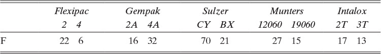
TABLE 10-4. F values (ft-1) for structured packings (Fair, 1985; Geankoplis, 2003)
where packing size factor Cp,size is given in Table 10-5, and δp is a characteristic packing dimension in inches. For random packing, δp = nominal size or diameter of the packing, and for structured packing, δp = height of the corrugation. Ceramic packings have thicker walls than plastic, and plastic has thicker walls than metal; thus, ceramic packings have the lowest free space, highest pressure drops, and highest F values. Generally, lower F values result in smaller column diameters. Figure 10-27 is not a perfect fit of all the data. Better results can be obtained using pressure drop curves measured for a given packing (e.g., see Kister et al., 2007). Specifically, predicted pressure drop for nonaqueous systems at high flow parameter values is too low (Kister and Gill, 1991).
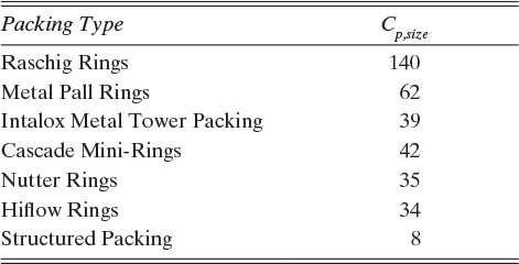
TABLE 10-5. Size factors for Eq. (10-38) (Bennett, 2000), copyright 2000, AIChE. Reproduced with permission of the American Institute of Chemical Engineers.
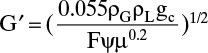
The Flooding curve in Figure 10-27 can be fit by the equation (Kessler and Wankat, 1988):

where µ is liquid viscosity in cp, ψ = ρwater/ρL, gc = 32.2, Flv [Eq. (10-9)] is abscissa of Figure 10-27, densities are mass densities, and L and G or WL and Wv are mass flow rates.
Below the flooding curves, the pressure drop can be correlated with an equation of the form

where Δp is pressure drop in inches of water per foot of packing, and L′ and G′ are fluxes in lb/s-ft2. Constants α and β are given in Table 10-3 for dumped packings (Ludwig, 1997). Alternative flooding and pressure drop correlations are given by Kister and Larson (1997), Kister et al. (2007), Ludwig (1997), and Strigle (1994).
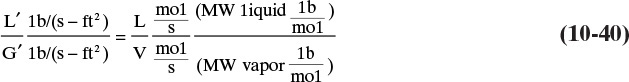
The generalized correlation in Figure 10-27 for Eqs. (10-39) is used as follows. The designer first picks a point in the column and determines gas and liquid densities (ρG and ρL), liquid viscosity (µ), value of ψ, and packing factor for the packing of interest. The ratio of liquid to vapor fluxes, L′/G′, is equal to internal reflux ratio, L/V, if liquid and vapor have the same composition because area terms divide out, and molecular weights cancel. If liquid and vapor mole fractions are significantly different at this point, then
In the first design method the designer chooses the pressure drop per unit length of packing. This number ranges from 0.1 to 0.4 in. of water/ft for vacuum columns, from 0.25 to 0.4 in. of water/ft for absorbers and strippers, and from 0.4 to 0.8 in. of water/ft for atmospheric and high-pressure columns (Coker, 1991). With the value of the abscissa and the parameter known, the ordinate can be determined. G′ is the only unknown in the ordinate. Once G′ is known, the area is
In the second design method, the flooding curve in Figure 10-27 or Eq. (10-39a) is used to determine G′flood. The actual operating vapor flux will be some percent of G′flood. The usual range is 65% to 90% of flooding with 70% to 80% being most common. Area is then determined from Eq. (10-41). The flooding correlation is not perfect. To have 95% confidence a safety factor of 1.32 is suggested for the calculated cross-sectional area (Bolles and Fair, 1982).
The diameter is easily calculated once the area is known. Since the liquid and vapor properties and gas and liquid flow rates all vary, diameter is determined at several locations, and the largest value is used. If there are significant variations in vapor flow rate, the largest diameter occurs where V is largest.
EXAMPLE 10-4. Packed column diameter calculation
A distillation column is separating n-hexane from n-heptane using 1-in. ceramic Intalox saddles. The allowable pressure drop in the column is 0.5 in. of water/ft. Average column pressure is 1.0 atm. Separation in the column is essentially complete, so the distillate is almost pure hexane, and the bottoms is almost pure heptane. The saturated liquid feed is 50.0 mol% n-hexane. L/V = 0.8. If F = 1000.0 lbmol/h and D = 500.0 lbmol/h, estimate the column diameter required at the top.
Solution
A. Define. Find diameter that gives Δp = 0.5 in. of water/ft at the top of the column.
B. Explore. Needed physical properties, most of which are in Examples 10-1 to 10-3:
n-Hexane: MW 86.17, bp 69°C = 342 K, ρL = 0.659 g/ml, viscosity (at 69°) = 0.22 cP
n-Heptane: MW 100.2, bp 98.4°C = 371.4 K, ρL = 0.684 g/ml, viscosity (at 98.4°) = 0.205 cP. Estimate vapor densities with ideal gas law, ρV = n(MWV)/V = p(MW)/RT.
Water density at 69°C = 0.9783 g/ml. We can use Figure 10-27 with F from Table 10-3 or Eq. (10-39b) with α and β from Table 10-3. We will compare the methods.
C. Plan. Figure 10-27 and Eq. (10-39b) can both be used to determine diameter.
D. Do it. The top is essentially pure n-hexane. Then
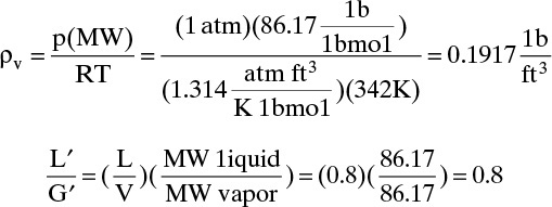
Abscissa for Figure 10-27 is
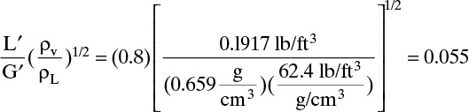
From Figure 10-27 at (Δp = 0.5), 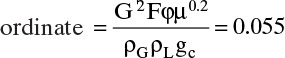
(Obtaining the same value for ordinate and abscissa is an accident!) Then
From Table 10-3, F = 98.0. Thus
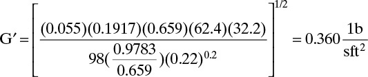
From Eq. (10-41), Area = (V lbmol/s)(MWV)/G′. V = L + D = (L/D + 1)D, where
This gives Area = (0.6944)(86.17)/(0.380) = 166.0 ft2 and
Diameter = (4.0 × Area/π)1/2 = (4.0 × 166.0/π)1/2 = 14.54 ft.
Alternative: Use Eq. (10-39b). First we must rearrange the equation. Since L′/G′ = L/V, have L′ = (L/V)G′. Then Eq. (10-39b) becomes

From Table 10-3, α = 0.52 and β = 0.16. Then the equation is
Using our previous answer, G′ = 0.360, as the first guess and using direct substitution, we obtain G′ = 0.404 as the solution in two trials. The equation is also easy to solve on a spreadsheet with Goal Seek. Then
Area = (V lbmol/s)(MWV)/G′ = (0.6944)(86.17)/(0.404) = 148.1 ft2 and
Diameter = (4.0 × Area/π)1/2 = (4.0 × 148.1/π)1/2 = 13.73 ft.
There is a 6% difference between this answer and the one we obtained graphically. Since α and β in Eqs. (10-39b) and (10-42) are specific for this packing and are not based on generalized curves, the lower value is probably more accurate, and a 14.0-ft diameter would be used. If we wanted to be conservative (safe), a 14.5-ft diameter would be used or additional safety factors (Fair, 1985) might be employed.
E. Check. Solving the problem two different ways is a good, but incomplete, check. The check is incomplete because the same values for several variables (e.g., ρG, V, and MW) were used in both solutions. Errors in these variables will not be evident in the comparison of the two solutions.
F. Generalize. Either Figure 10-27 or Eq. (10-39b) can be used for pressure drop calculations in packed beds. The use of both is a good check procedure the first time you calculate a diameter (or Δp). Remember, the required diameter also must be estimated at other locations in the column. A common alternate design procedure is to use Figure 10-27 with the same packing at 75% of flooding. This design requires a diameter of 12.4 ft and has a pressure drop of approximately 1.5 in. of water per foot of packing (0.37 kPa/ft). We can also compare with Example 10-2, which designed a sieve tray column for the same separation. At 75% of flooding the sieve tray was 11.03 ft in diameter. The packed column is a larger diameter because a small packing is used. If a larger-diameter packing were used, the packed column diameter could be smaller. The effect of location on the calculated column diameter is explored in Problem 10.D17. If pressure drop is absolutely critical, the column area should be multiplied by a safety factor of 2.2 (Bolles and Fair, 1982).
There are three alternatives that can overcome the flooding limitations of countercurrent packed columns. The rotating packed bed or Higee process (Agarwal et al., 2010; Lin et al., 2003; Ramshaw, 1983) puts the packing inside an annular-flow column that is rotated at high rpm. This device achieves high rates of mass transfer, and because of the effective increase in gravity, it floods at much higher velocities. The column size is considerably smaller than for normal distillation and absorption systems, but the device is more complicated. A few commercial units have been built. The second approach is to do absorption, stripping, or extraction in countercurrent flow with hollow fiber membrane phase contactors (Humphrey and Keller, 1997; Reed et al., 1995). One phase flows inside the hollow fibers and the other flows countercurrent to it in the shell. High flow rates are observed because flooding is unlikely, and relatively low HETP values have been reported because of the very large surface area of hollow fibers. The third approach is to avoid countercurrent operation altogether and operate in cocurrent flow where there is no flooding (see Section 12.8).
10.11 Economic Trade-Offs for Packed Columns
In the design of a packed column designers have many trade-offs that are ultimately reflected in operating and capital costs. After deciding that a packed column will be used instead of a staged column, designers must choose the packing type. There is no single packing that is most economical for all separations. For most distillation systems the more efficient packings (low HETP and low F) are also most expensive per volume but may be cheaper overall. Designers must then pick the material of construction. Since random commercial packings of the same size all have an HETP in the range of 1 to 2 ft, the major difference between them is the packing factor, F. Perusal of Table 10-3 shows that there is a very large effect of packing size and a lesser but still up to fourfold effect of packing type on F value. The material of construction can also change F by a factor that can be as high as 3. From Figure 10-27,

A fourfold increase in F would cause a halving of G′ and a doubling of the required area [Eq. (10-41)]. The diameter can then be calculated:
Note that F is the packing factor, not the feed rate! Thus, the major advantage of more efficient packings, structured packings, and the larger-size packings is that they can be used with a smaller-diameter column, which is not only less expensive but requires less packing.
At this point, designers pick the packing size and determine both the HETP and the packing factor. Larger-size packing has a larger HETP (requires a larger height) but a smaller F factor and hence a smaller diameter. Thus, there is a trade-off between packing sizes. The larger-size packings are cheaper per cubic foot but cannot be used in very small-diameter columns because of excessive channeling. As a rule of thumb
Structured packings are purchased for the desired diameter column and are not restrained by Eq. (10-45). In small-diameter columns (say, less than 6 in.), structured packings allow low F factors and hence low Δp without violating Eq. (10-45).
Pressure drop per foot or the fraction of flooding is also selected. Operating costs in absorbers and strippers increase as Δp/ft increases, but the diameter decreases and hence capital costs for the column decrease. Operation should be in the range of 20% to 90% of flood and is usually in the range of 65% to 90% of flooding. Since columns are often made in standard diameters, the pressure drop per foot is usually adjusted to give a standard-size column.
In many applications packed columns appear to be the wave of the future. Columns packed with structured packings have a combination of low pressure drop and high efficiency that often makes them less expensive than either randomly packed columns or staged columns. Random packings can be made in a wide variety of materials so that practically any chemical can be processed. Many of the flow distribution problems that limited the size of packed columns in the past appear to have been solved.
10.12 Choice of Column Type
You are a young engineer asked to design a distillation column. Do you use trays, random packing, or structured packing? Kister et al. (1994) considered which column to use in considerable detail.
Vacuum columns, particularly high vacuum, are typically used when thermal degradation or polymerization occur at the boiling temperatures at atmospheric pressure. Since we must have upward flow of vapor, the reboiler has to be at a higher pressure than the condenser, which is connected to the vacuum pump. Thus,
The lower pressure drop of structured packing, specifically wire gauze packings, is a major advantage if thermal degradation or polymerization is a problem (Olujic, 2014). The reboiler will be at a lower pressure in a packed column and as a result will be at a lower temperature. In addition, lower pressure in the reboiler increases the relative volatility, which can allow for a lower reflux ratio. One negative to lower pressure is the corresponding drop in vapor density [see Eq. (10-15)] that will increase the required column diameter. The lower pressure drop of structured packing is also an advantage for cryogenic distillation of argon from air because at lower pressures, the relative volatility for the argon-oxygen separation is larger (Agrawal and Woodward, 1991).
For atmospheric and pressure columns, pressure drop is usually relatively unimportant, and you need to compare optimally designed tray columns to optimally packed columns. An optimally designed tray column balances tray and downcomer areas so that both restrict capacity simultaneously. An optimally designed packed column has good liquid and vapor distribution, and capacity restrictions are due to the inherent qualities of the packing, not the supports or the distributors.
Kister et al. (1994) compared a large amount of data generated by FRI in a 4.0-ft diameter column and for the structured packing at p < 90 psia by the Separation Research Program (SRP) at the University of Texas-Austin in a 17-in. diameter column. Nutter rings were chosen to represent state-of-the-art random packings. The only structured packing measured at high pressures is Norton’s Intalox 2T, which was chosen to represent structured packing. Test data were available on both sieve and valve trays with 24-in. tray spacing. All comparisons were at total reflux. For efficiency they compared practical HETP values that include height consumed by distribution and redistribution equipment.
where multiplier M > 1. For 2-in. random packing M = 1.1, while for structured packing (Intalox 2T) M = 1.2. For trays
where S is the tray spacing in inches, and Eo is the fractional overall efficiency. For capacity they compared the capacity factor at flooding:
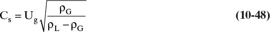
where Ug is the gas velocity in ft/s, and the densities are mass densities. Both efficiency and capacity results were plotted against the flow parameter (FP) given in Eq. (10-9) and repeated here.

Since valve trays were superior to sieve trays (higher Cs,flood and lower HETPtray), valve trays were compared to packings. Overall comparison of tray and packing efficiencies (as measured by adjusted HETP) is shown in Figure 10-28. Adjusted HETP for structured packing is lower over most of the FP range, while HETPs for trays and random packings are almost identical. At high FP values (high pressures) random packing had the lowest HETP, and structured packing the highest. Capacities, as measured by Cs,flood values, are compared in Figure 10-29. At low FP (low pressures) structured packing has a 30% to 40% advantage in capacity. At FP values around 0.2 all devices have similar capacities. At high pressures (high FP values) trays clearly had higher capacities.

FIGURE 10-28. Overall comparison of efficiency of trays, random packing, and structured packing (Kister et al., 1994). Reprinted with permission from Chemical Engineering Progress, copyright AICHE 1994
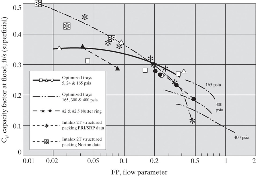
FIGURE 10-29. Overall comparison of capacity of trays, random packing, and structured packing (Kister et al., 1994). Reprinted with permission from Chemical Engineering Progress, copyright AICHE 1994
In addition to efficiency and capacity, engineers need to be vitally concerned with safety. Many fires are related to distillation and absorption columns. The most dangerous periods are during abnormal operation—upsets, shutdowns, maintenance, total reflux operation, and startups. Structured packing has been implicated in a number of fires, mainly occurring during shutdown and maintenance of units (Ender and Laird, 2003). Several different mechanisms were identified. (1) Hydrocarbons may coat the packing with a thin film that is very difficult to remove. If the packing is at an elevated temperature when it is exposed to air, the hydrocarbons may self-ignite. (2) Coke or polymers may form on the packing during normal operation. Although coking or polymerization will eventually be signaled by increased pressure drop, a large fraction of the bed will contain coke or polymer by the time this is noticed. Cooling the interior of the coke or polymer is very difficult because the thermal conductivity is low. Thus, the interior of the coke or polymer may be much hotter than the vapor, which is where the temperature-measuring device is located. When the column is opened to air, the coke or polymer may catch fire. (3) If sulfur is present in the feed, corrosion of carbon steel components up- or downstream of the column can form iron sulfide (FeS) that can settle on the packing. Iron sulfide is difficult to remove and will autoignite at ambient temperature when exposed to air. (4) Packing usually arrives from the factory coated with lubricating oil that can catch fire if hot work (e.g., welding) is conducted on the column. (5) If the hydrocarbons, coke, or FeS on the packing catches fire, the very thin metal packing can burn. This is more likely with reactive metals such as aluminum, titanium, and zirconium. The danger of metal fires is because they burn at very high temperatures (up to 1500°C), they can be very destructive.
Standard operating procedures should be designed to prevent fires (Ender and Laird, 2003).
1. Cool the column to ambient temperature before opening it. Continuously monitor temperature.
2. Wash the column extensively to remove residues and deposits.
3. If sulfur is present in the feed, assume FeS formed, and wash the column with permanganate or percarbonate.
4. Purge with inert gas (nitrogen, carbon dioxide, or steam), and be sure personnel are equipped with respirators before opening columns.
5. Minimize the number of open manways to reduce air entry and allow for rapid closure of the column if there is a fire. Do not force air into the column. This may sound counterintuitive since air circulation will help cool the column if there is no fire; however, fires can be prevented or stopped by starving them of oxygen.
Ultimately, the decision of which column design to use is often economic. Currently, unless there are exceptional circumstances, it appears that structured packings are most economical in low-pressure operation, and valve trays are most economical in high-pressure operation. At atmospheric and slightly elevated pressures structured packings have efficiency but not capacity advantage; however, structured packings are often considerably more expensive than valve trays (Humphrey and Keller, 1997). The slight added safety risk of structured packing with flammable materials also needs to be considered. Thus, random packings (small-diameter columns) and valve trays will often be preferred for atmospheric and slightly elevated pressures. Exceptional circumstances include the need to use exotic materials such as ceramics, which favors random packings and the need for high holdup for reactive systems, which favors trays. Packed columns are dynamically more stable than staged columns. They are less likely to fail during startup, shutdown, and other upsets in operation. This is particularly true of absorption and stripping columns (Gunaseelan and Wankat, 2002) and should be considered if the column will be used for processing vent gases in emergencies. Note that tray columns still retain advantages in addition to cost for a number of applications such as very large column diameters, columns with multiple drawoffs, varying feed compositions, highly fouling systems, and systems with solids in which sieve trays are usually used (Anon., 2005).
References
Agarwal, L., V. Pavani, D. P. Rao, and N. Kaistha, “Process Intensification in HiGee Absorption and Distillation: Design Procedure and Applications,” Ind. Engr. Chem. Research, 49, pp. 10046–10058 (2010).
Agrawal, R., and D. W. Woodward, “Impact of Structured Packing on Distillation of Argon from Air,” XVIIIth International Congress of Refrigeration, Montreal, Quebec, Canada, paper 34, August 10–17, 1991.
Anon., “Facts at Your Fingertips,” Chemical Engineering, 59 (April 2005).
Bennett, D. L., “Optimize Distillation Columns. Part II. Packed Columns,” Chem. Engr. Progress, 96 (5), 27 (2000).
Biegler, L. T., I. E. Grossman, and A. W. Westerberg, Systematic Methods of Chemical Process Design, Prentice Hall, Upper Saddle River, NJ, 1997.
Bolles, W. L., Pet. Refiner., 25, 613 (1946).
Bolles, W. L., “Tray Hydraulics, Bubble-Cap Trays,” in B. D. Smith (Ed.), Design of Equilibrium Stage Processes, McGraw-Hill, New York, 1963, Chapter 14.
Bolles, W. L., “Estimating Valve Tray Performance,” Chem. Eng. Prog., 72 (9), 43 (September 1976).
Bolles, W. L., and J. R. Fair, “Improved Mass-Transfer Model Enhances Packed-Column Design,” Chem. Eng., 89 (14), 109 (July 12, 1982).
Bonilla, J. A., “Don’t Neglect Liquid Distributors,” Chem. Engr. Prog., 89 (3), 47 (March 1993).
Coker, A. K., “Understand the Basics of Packed-Column Design,” Chem. Engr. Progress, 87 (11), 93 (November 1991).
Dean, J. A., Lange’s Handbook of Chemistry, 13th ed., McGraw-Hill, New York, 1985.
Eckert, J. S., “Selecting the Proper Distillation Column Packing,” Chem. Eng. Prog., 66 (3), 39 (1970).
Eckert, J. S., “Design of Packed Columns,” in P. A. Schweitzer (Ed.), Handbook of Separation Techniques for Chemical Engineers, McGraw-Hill, New York, 1979, Section 1.7.
Ellis, S. R. M., and F. Brooks, “Performance of Packed Distillation Columns Under Finite Reflux Conditions,” Birmingham Univ. Chem. Eng., 22, 113 (1971).
Ender, C., and D. Laird, “Minimize the Risk of Fire during Column Maintenance,” Chem. Engr. Progress, 99 (9), 54 (September 2003).
Fair, J. R., “Tray Hydraulics: Perforated Trays,” in B. D. Smith, Design of Equilibrium Stage Processes, McGraw-Hill, New York, 1963, Chapter 15.
Fair, J. R., “Gas-Liquid Contacting,” in R. H. Perry and D. Green (Eds.), Perry’s Chemical Engineer’s Handbook, 6th ed., McGraw-Hill, New York, 1984, Section 18.
Fair, J. R., “Stagewise Mass Transfer Processes,” in A. Bisio and R. L. Kabel (Eds.), Scaleup of Chemical Processes, Wiley, New York, 1985, Chapter 12.
Fair, J. R., H. R. Null, and W. L. Bolles, “Scale-up of Plate Efficiency from Laboratory Oldershaw Data,” Ind. Eng. Chem. Process Des. Develop., 22, 53 (1983).
Fair, J. R., and R. L. Matthews, “Better Estimate of Entrainment from Bubble Caps,” Pet. Refiner., 37 (4), 153 (1958).
Furter, W. F., and W. T. Newstead, “Comparative Performance of Packings for Gas-Liquid Contacting Columns,” Can. J. Chem. Eng., 51, 326 (1973).
Geankoplis, C. J., Transport Processes and Separation Process Principles, 4th ed., Prentice Hall, Upper Saddle River, NJ, 2003.
Glitsch, Inc., Ballast Tray Design Manual, Glitsch, Inc., Dallas, TX, 1974.
Glitsch, Inc., “17 Critical Questions and Answers about Trays, Column Internals, and Accessories,” Glitsch, Inc., Dallas, TX, 1985.
Green, D. H, and R. H. Perry (Eds.), Perry’s Chemical Engineers’ Handbook, 8th ed., McGraw-Hill, New York, 2008.
Gunaseelan, P., and P. C. Wankat, “Transient Pressure and Flow Predictions for Concentrated Packed Absorbers Using a Dynamic Non-Equilibrium Model,” Ind. Engr. Chem. Research, 41, 5775 (2002).
Huang, C.-J., and J. R. Hodson, “Perforated Trays,” Pet. Refiner., 37 (2), 104 (1958).
Hughmark, G. A., and H. E. O’Connell, “Design of Perforated Plate Fractionating Towers,” Chem. Eng. Prog., 53, 127-M (1957).
Humphrey, J. L., and G. E. Keller II, Separation Process Technology, McGraw-Hill, New York, 1997.
Jones, E. A., and M. E. Mellbom, “Fractionating Column Economics,” Chem. Eng. Prog., 75 (5), 52 (1982).
Jones, W. E., and J. A. Wilson, “Changing Vapor-Liquid Traffic in a Distillation Column,” Chem. Eng. Educ., 30 (1), 36 (1996).
Kessler, D. P., and P. C. Wankat, “Correlations for Column Parameters,” Chem. Eng., 71 (September 26, 1988).
Kister, H. Z., “Guidelines for Designing Distillation—Column Intervals,” Chem. Eng., 87 (10), 138 (1980a).
Kister, H. Z., “Outlets and Internal Devices for Distillation Columns,” Chem. Eng., 87 (15), 79 (1980b).
Kister, H. Z., “Design and Layout for Sieve and Valve Trays,” Chem. Eng., 87 (18), 119 (1980c).
Kister, H. Z., “Mechanical Requirements for Sieve and Valve Trays,” Chem. Eng., 87 (23), 283 (1980d).
Kister, H. Z., “Downcomer Design for Distillation Tray Columns,” Chem. Eng., 87 (26), 55 (1980e).
Kister, H. Z., “Inspection Assures Trouble-Free Operation,” Chem. Eng., 88 (3), 107 (1981a).
Kister, H. Z., “How to Prepare and Test Columns Before Startup,” Chem. Eng., 88 (7), 97 (1981b).
Kister, H. Z., Distillation Operation, McGraw-Hill, New York, 1990.
Kister, H. Z., Distillation Design, McGraw-Hill, New York, 1992.
Kister, H. Z., Distillation Troubleshooting, McGraw-Hill, New York, 2005.
Kister, H. Z., “Effects of Design on Tray Efficiency in Commercial Towers,” Chem. Engr. Progress, 104 (6), 39 (June 2008).
Kister, H. Z., R. Dionne, W. J. Stupin, and M. R. Olsson, “Preventing Maldistribution in Multi-Pass Trays,” Chem. Engr. Progress, 106 (4), 32 (April 2010).
Kister, H. Z., and D. F. Gill, “Predict Flood Point and Pressure Drop for Modern Random Packings,” Chem. Engr. Progress, 87 (2), 32 (February 1991).
Kister, H. Z., and K. F. Larson, “Packed Distillation Tower Design,” in P. A. Schweitzer (Ed.), Handbook of Separation Techniques for Chemical Engineers, 3rd ed., McGraw-Hill, New York, 1997, Section 1.6.
Kister, H. Z., K. F. Larson, and T. Yanagi, “How Do Trays and Packings Stack Up?” Chem. Engr. Progress, 90 (2), 23 (February 1994).
Kister, H. Z., J. Scherffius, K. Afshar, and E. Abkar, “Realistically Predict Capacity and Pressure Drop for Packed Columns,” Chem. Eng., 28 (7), 28 (July 2007).
Koch Engineering Co., Design Manual Flexitray, Koch Engineering Co., Wichita, KS, 1982.
Larson, K. F., and H. Z. Kister, “Distillation Tray Design,” in P. A. Schweitzer (Ed.), Handbook of Separation Techniques for Chemical Engineers, 3rd ed., McGraw-Hill, New York, 1997, Section 1.5.
Lieberman, N. P., and E. T. Lieberman, A Working Guide to Process Equipment, 3rd ed., McGraw-Hill, New York, 2008.
Lin, C.-C., W.-T. Liu, and C.-S. Tan, “Removal of Carbon Dioxide by Absorption in a Rotating Packed Bed,” Ind. Engr. Chem. Res., 42, 2381 (2003).
Lockett, M. J., Distillation Tray Fundamentals, Cambridge University Press, Cambridge, UK, 1986.
Ludwig, E. E., Applied Process Design for Chemical and Petrochemical Plants, Vol. 2, 2nd ed., Gulf Pub. Co., Houston, 1997.
Murch, D. P., “Height of Equivalent Theoretical Plate in Packed Fractionation Columns,” Ind. Eng. Chem., 45, 2616 (1953).
O’Brien, D., and M. A. Schulz, “Ask the Experts: Distillation,” Chem. Engr. Progress, 100 (2), 14 (February 2004).
O’Connell, H. E., “Plate Efficiency of Fractionating Columns and Absorbers,” Trans. Amer. Inst. Chem. Eng., 42, 741 (1946).
Olujic, Z., “Vacuum and High-Pressure Distillation,” in A. Gorak and Z. Olujic (Eds.), Distillation Equipment and Processes, Academic Press, London, 2014, Chapter 9.
Perry, R. H., C. H. Chilton, and S. D. Kirkpatrick (Eds.), Chemical Engineer’s Handbook, 4th ed., McGraw-Hill, New York, 1963.
Perry, R. H., and D. W. Green (Eds.), Perry’s Chemical Engineers’ Handbook, 6th ed., McGraw-Hill, New York, 1984.
Perry, R. H., and D. W. Green (Eds.), Perry’s Chemical Engineers’ Handbook, 7th ed., McGraw-Hill, New York, 1997.
Pilling, M., “Ensure Proper Design and Operation of Multi-Pass Trays,” Chem. Engr. Progress, 101 (6), 22 (June 2005).
Pilling, M., and D. R. Summers, “Be Smart about Column Design,” Chem. Engr. Progress, 108 (11), 32 (November 2012).
Poling, B. E., J. M. Prausnitz, and J. P. O’Connell, The Properties of Gases and Liquids, 5th ed., McGraw-Hill, New York, 2001.
Peters, W. A., “The Efficiency and Capacity of Fractionating Columns,” Ind. Eng. Chem., 14, 476 (1922).
Ramshaw, C., “Higee Distillation—An Example of Process Intensification,” Chem. Engr., 389, 13 (1983).
Reed, B. W., et al., “Membrane Contactors,” in R. D. Noble and S. A. Stern (Eds.), Membrane Separations Technology—Principles and Applications, Elsevier, 1995, Chapter 10.
Reid, R. C., J. M. Prausnitz, and T. K. Sherwood, The Properties of Gases and Liquids, 3rd ed., McGraw-Hill, New York, 1977.
Seider, W. D., J. D. Seader, D. R. Lewin, and S. Widago, Product and Process Design Principles, 3rd ed., Wiley, New York, 2009.
Sherwood, T. K., G. H. Shipley, and F. A. L. Holloway, “Flooding Velocities in Packed Columns,” Ind. Eng. Chem., 30, 765 (1938).
Sherwood, T. K., R. L. Pigford, and C. R. Wilke, Mass Transfer, McGraw-Hill, New York, 1975.
Sloley, A. W., “Avoid Problems during Distillation Column Startups,” “Chem. Engr. Progress, 92 (7), 30 (July 1996).
Smith, B. D., Design of Equilibrium Stage Processes, McGraw-Hill, New York, 1963.
Smith, B. D., and R. Srivastava, Thermodynamic Data for Pure Compounds, Elsevier, Amsterdam, 1986.
Stephan, K., and H. Hildwein, Recommended Data of Selected Compounds and Binary Mixtures: Tables, Diagrams and Correlations, DECHEMA, Frankfurt am Main, Germany, 1987.
Strigle Jr., R. F., Packed Tower Design and Applications: Random and Structured Packings, 2nd ed., Gulf Publishing Co., Houston, 1994.
Torzewski, K. (Dept. Ed.), “Facts at Your Fingertips, Tray Column Design,” Chemical Engineering, 116 (1), 17 (January 2009).
Walas, S. M., Chemical Process Equipment: Selection and Design, Butterworth, Boston, 1988.
Wang, G. Q., X. G. Yuan, and K. T. Yu, “Review of Mass-Transfer Correlations for Packed Columns,” Ind. Engr. Chem. Res., 44, 8715 (2005).
Wankat, P. C., “Balancing Diameters of Distillation Column with Vapor Feeds,” Ind. Engr. Chem. Research, 46, pp. 8813–8826 (2007a).
Wankat, P. C., “Reducing Diameters of Distillation Column with Largest Calculated Diameter at the Bottom,” Ind. Engr Chem. Research, 46, pp. 9223–9231 (2007b).
Wankat, P. C., “Decreasing Costs of Distillation Columns with Vapor Feeds,” Chem. Eng. Sci., 137, pp. 955–963 (2015).
Whitt, F. R., “A Correlation for Absorption Column Packing,” Brit. Chem. Eng., July, 1959, p. 395.
Woods, D. R., Rules of Thumb in Engineering Practice, Wiley-VCH, Weinheim, 2007.
Zenz, F. A., “Design of Gas Absorption Towers,” in P. A. Schweitzer (Ed.), Handbook of Separation Techniques for Chemical Engineers, 3rd ed., McGraw-Hill, New York, 1997, Section 3.2.
Homework
A. Discussion Problems
A1. What effect does increasing the spacing between trays have on:
a. Column efficiency?
b. Csb,f and column diameter?
c. Column height?
d. Maintenance?
A2. Several different column areas are used in this chapter. Define and contrast: total cross-sectional area, net area, downcomer area, active area, and hole area.
A3. Calculate the pressure drop in kPa from the head of clear liquid.
A4. Another type of weir not shown in Figure 10-6 is the adjustable weir. In an adjustable weir the height can be changed by loosening bolts, moving the weir, and retightening the bolts. List as many reasons as you can think of why this type of weir is generally not recommended.
A5. As shown by the Leaning Tower of Pisa, towers that do not have a proper footing can develop a significant lean. Even if a distillation tower is structurally sound, leaning away from being vertical affects the operation. What is likely to go wrong for a tray tower if it leans?
A6. Valve trays are often constructed with two different weight valves. What would this do to Figure 12-21? What are the probable advantages of this design?
A7. Beer stills are distillation columns that process the raw feed from fermentation. This feed includes cells and cell debris in addition to ethanol and water. Why are sieve plates with larger-than-normal holes the preferred column internals for beer stills?
A8. Intermediate feeds should not be introduced into a downcomer. Explain why.
A9. What are the characteristics of a good packing? Why are marbles a poor packing material?
A10. Develop your key relations chart for this chapter.
A11. If HETP varies significantly with the gas rate, how would you design a packed column?
A12. Structured packings work very well in vacuum and atmospheric pressure distillation columns, but sometimes structured packings do not work well in high-pressure columns. What is different about operation at high pressure that may make the structured packings not work as well?
A13. What effect will an increase in viscosity have on pressure drop in a packed column?
A14. Refer to Table 10-3.
a. Which is more desirable, a high or low packing factor, F?
b. As packing size increases, does F increase or decrease? What is the functional form of this change (e.g., linear, quadratic, cubic)?
c. Why do ceramic packings have higher F factors than plastic or metal packings of the same type and size? When would you choose a ceramic packing?
A15. Why can large-size packings not be used in small-diameter columns? What is the reason for the rule of thumb given in Eq. (10-45)?
A16. We have designed a sieve tray distillation column for p = 3.0 atm. We decide to look at the design for p = 1.0 atm. Assume feed flow rate, mole fractions in the feed, and L/D are the same for both designs. The feed is a saturated liquid for both designs. We want the same recoveries of light and heavy key for both designs. Both designs have a total condenser and a partial reboiler. Compared to the original design at 3.0 atm, the design at 1.0 atm will
1. Have
a. fewer stages.
b. more stages.
c. the same number of stages.
2. Require
a. a smaller-diameter column.
b. a larger-diameter column.
c. the same column diameter.
3. Have
a. lower reboiler temperature.
b. higher reboiler temperature.
c. the same reboiler temperature.
A17. Distillation columns have been installed on ships. What are the likely effects of the ship’s motion on the performance of the distillation column? Would you recommend use of random packing, structured packing, or a tray column?
A18. Designing, constructing, and operating distillation columns require teamwork. What roles do chemical engineers, mechanical engineers, civil engineers, electrical engineers, and material engineers take?
B. Generation of Alternatives
B1. One type of valve is shown in Figure 10-1. Brainstorm alternative ways in which valves could be designed.
B2. What other ways of contacting in packed columns can you think of?
a. A farmer friend of yours is going to build his own distillation system to purify ethanol made by fermentation. He wants to make his own packing. Suggest 30 different things he could make or buy cheaply to use as packing (set up a brainstorming group to do this—make no judgments as you list ideas).
b. Look at your list in part a. Which idea is the craziest? Use this idea as a trigger to come up with 20 more ideas (some of which may be reasonable).
c. Go through your two lists from parts a and b. Which ideas are technically feasible? Which ideas are also cheap and durable? List about 10 ideas that look like the best for further exploration.
B4. If trays are good, random packing is good, and structured packing is good, why not combine them? Think of at least ten ways you might do this.
C. Derivations
C1. You need to temporarily increase the feed rate to an existing column without flooding. Since the column is now operating at about 90% of flooding, you must vary some operating parameter. The column has 0.4572 m tray spacing, is operating at 1.0 atm, and has a flow parameter of
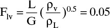
The column is rated for a total pressure of 10 atm. L/D = constant. The relative volatility for this system decreases very slowly as pressure increases. The condenser and reboiler can easily handle operation at a higher pressure. Downcomers are large enough for larger flow rates. Will increasing the column pressure increase the feed rate that can be processed? It is likely that
Determine the value of the exponent for this situation. Use the ideal gas law.
C2. Show that staged column diameter is proportional to (feed rate)1/2 and to (1 + L/D)1/2.
C3. If the packing factor were unknown, you could measure Δp at a series of gas flow rates. How would you determine F from these data?
C4. Using a McCabe-Thiele diagram for a binary system, show why the purity will be reduced compared to the base case if N and L/D are constant and one of the diameter balancing methods in Figure 10-18 (base case is a saturated vapor feed) or Figure 10-19 (base case is a saturated liquid feed) is used to reduce the column volume. Although this demonstration is for a binary system, the logic is true for multicomponent systems also.
C5. Using a McCabe-Thiele diagram for a binary system, show why increasing N may not be sufficient to keep constant purity compared to the base case if the diameter balancing method in Figure 10-18A (base case is a saturated vapor feed) or 10-19A (base case is a saturated liquid feed) is used to reduce the column volume. Although this demonstration is for a binary system, the logic is true for multicomponent systems also.
C6. Derive Eq. (10-15) for an ideal gas.
D. Problems
*Answers to problems with an asterisk are at the back of the book.
D1.* Repeat Example 10-1 for an average column pressure of 700.0 kPa.
D2.* Repeat Example 10-2, except calculate the diameter at the bottom of the column. For n-heptane: MW = 100.2, bp 98.4°C, sp gravity = 0.684, viscosity (98.4°C) = 0.205 cP, σ (98.4°C) = 12.5 dynes/cm.
D3. The calculations in Example 10-3 were done for conditions at the top of the column. Physical properties will vary throughout the column, but columns are normally constructed with identical trays, downcomers, weirs, etc., on every stage (this is simpler and cheaper). For a 12-ft diameter column, calculate entrainment, pressure drops, downcomer residence time, and weeping at the bottom of the column. The results of Problem 10.D2 are required. If the column will not operate, will it work if the gap between the tray and the downcomer apron is increased to 1.5 in.?
D4.* We wish to repeat the distillation in Examples 10-2 and 10-3 except using valve trays. The valves have a 2-in. diameter head. For the top of the column, estimate the pressure drop vs. hole velocity curve. Assume that Kv and Cv values are the same as in Figure 10-21. Each valve weighs approximately 0.08 lb.
D5. Repeat Example 10-2 except calculate the diameter at the bottom of the column at a pressure of 700.0 kPa. The surface tension of pure n-heptane at 20°C is 20.14 dynes/cm (0.0214 N/m), and the temperature coefficient is –0.0980 dynes/cm/K (www.surface-tension.de). Use the DePriester chart to estimate bottoms temperature.
D6.* We are testing a new packing for separation of benzene and toluene. The column is packed with 3.5 m of packing and has a total condenser and a partial reboiler. Operation is at 760.0 mm Hg, where α varies from 2.61 for pure benzene to 2.315 for pure toluene (Perry et al., 1963, p. 13–3). At total reflux we measure a benzene mole fraction of 0.987 in the condenser and 0.008 in the reboiler liquid. Find HETP:
a. Using α = 2.315.
b. Using α = 2.61.
c. Using a geometric average α.
Use either the Fenske equation or a McCabe-Thiele diagram.
D7. You have designed a sieve tray column with 0.3048-m tray spacing to operate at a pressure of 1.0 atm. The value of the flow parameter is Flv = 0.090, and the flooding velocity was calculated as 1.83 m/s. Unfortunately, your boss dislikes your design. She thinks that 0.3048-m tray spacing is not enough and that your reflux ratio is too low. You must redesign for a 0.6096-m tray spacing and increase L/V by 11%. Estimate the new flooding velocity.
Assumptions: Ideal gas, σ, ρL, and ρG are unchanged.
D8. A sieve tray column with 0.4572-m tray spacing is designed to operate at p = 2.0 atm. The value of the flow parameter is Flv = 0.5, and the flooding velocity was calculated as uflood = 1.83 m/s. Unfortunately, the latest lab results show that the distillation temperature is too high, and unacceptable thermal degradation occurs. To reduce the operating temperature, you plan to reduce the column pressure to 0.5 atm. Estimate the new flooding velocity.
Assumptions: Ideal gas, σ, and ρL are unchanged, ρL >> ρV (thus, ρL – ρV = ρL). Ignore the effect of temperature change in calculation of ρV.
D9.* 1000.0 kmol/h of a saturated vapor feed that is 60.0 mol% methanol and 40.0 mol% water is distilled in a sieve plate column operating at 75.0% of flooding velocity. Distillate is 99.9 mol% methanol, and bottoms is 1.0 mol% methanol. L/V = 0.6 and p = 1.0 atm. Use a 0.4572 m tray spacing and η = 0.90. Density of pure liquid methanol is 0.79 g/ml. Data are available in Table 2-7 and Problem 10.D22. Assume an ideal gas. The surface tension of pure methanol can be estimated as σ = 24.0 – 0.0773 T with T in °C (Dean, 1985, pp. 10–110). Calculate the diameter based on the conditions at the top of the column.
D10. The effect of liquid maldistribution in packed columns can be explored with a McCabe-Thiele diagram. Assume that a packed distillation column is separating a saturated liquid binary feed that is 40.0 mol% MVC. A distillate product, D = 100.0 kmol/h, that is 90.0% MVC is desired. Relative volatility = 3.0 and is constant. We operate at an L/D = 2(L/D)min. If there is liquid maldistribution, the actual L/V represents an average for the entire column. Assume that vapor is equally distributed throughout the column, but there is more liquid on one side than the other. The slope of the operating line on the low liquid side will be Llow/V not (L/V)avg. If the low liquid flow rate is small enough, the operating line on the low side will be pinched at the feed point, and the desired separation will not be obtained. What fraction of the average liquid flow rate must the low liquid flow rate be to just pinch at the feed concentration? Then generalize your result for L/D = M × (L/D)min, where M > 1.
D11. We wish to distill an ethanol-water mixture to produce 2250.0 lb of distillate product per day. The distillate product is 80.0 mol% ethanol and 20.0 mol% water. L/D = 2.0, and p = 1.0 atm. Your boss suggests trying a packed column with 1.0-in. plastic Pall rings. Calculate the diameter at the top of the column.
Physical properties: MWE = 46, MWW = 18, assume ideal gas, µL = 0.52 cP at 176°F, ρL = 0.82 g/ml.
a. Operation is at 75% of flooding. What diameter is required?
b.* If Eq. (10-45) is not satisfied, what size of plastic Pall rings should be used?
c.* Operation is at a pressure drop of 0.25 in. of water per foot of packing. Use the size of Pall rings found in part b. What column diameter is required?
d. Repeat part a (with 1.0-in. Pall rings) but for 22,500 lb of distillate product per day. If Eq. (10-45) is not satisfied, find the diameter of plastic Pall rings that work.
e. Note: It is not necessary to redo the entire calculation, since D and hence V and hence diameter are related to the feed rate.
D12. 10.0 kmol/h of a saturated vapor feed that is 23.5 mol% water with the remainder nitromethane is sent to an enricher that is packed with 1.524 m of packing. L/V = 0.8. The overhead vapor from the column is condensed and sent to a liquid-liquid settler. The water-rich layer is the distillate product xD = xβ = 91.4 mol% water. The nitromethane-rich layer from the settler is refluxed to the column. Find HETP in feet and water mole fraction in bottoms. Water-nitromethane data are given in Problem 8.E1.
D13. Repeat Problem 10.D9, calculating the diameter at the top, but condense the feed to a saturated liquid. Determine (L/D)min and L/D = M × (L/D)min with the same M value used in Problem 10.D9. Compare the diameter of this column to the diameter of 10.27 ft calculated for Problem 10.D9. Calculate the ratio QR,liquid_feed/QR,vapor_feed for this problem.
D14. a. We are distilling methanol and water in a column packed with 1-in. ceramic Berl saddles. The bottoms composition is 0.01 mol% methanol. The column operates at 1.0 atm pressure. The feed to the column is a saturated liquid at 1000.0 kmol/day and is 40.0 mol% methanol. L/D = 2.0. The distillate product is 99.8 mol% methanol. If we will operate at a vapor flow rate that is 80.0% of flooding, calculate the diameter based on conditions at the bottom of the column. Data are available in Tables 2-7 and 10-3. Vapor is an ideal gas. Viscosity of water at 100.0°C is 0.26 cP.
b. Suppose we wanted to use 1-in. plastic Intalox saddles. What diameter is required?
c. Note: Part b can be done in one line once part a is finished.
D15. Repeat Problem 10.D14a, except determine the diameter of a sieve plate column operating at 80.0% of flooding velocity. Use a 0.3048-m tray spacing and η = 0.85. The liquid surface tension of pure water is σ = 58.9 dynes/cm at 100.0°C.
D16. Repeat Example 10-4, except use 1/2-in. Intalox saddles. This calculation can be done without repeating the entire calculation in Example 10-4.
D17.* Repeat Example 10-4, except calculate the diameter at the bottom of the column.
D18. You have designed a packed column at 1.0 atm. The flow parameter Flv has a value of 0.2. The calculated gas flux at flooding is 0.50 lbm/[(s)(ft2)]. Your boss now wants to increase the column pressure to 4.0 atm. Assume that the vapor in the column follows the ideal gas law. What is the new gas flux at flooding?
D19. Repeat Problems 10.D9 and 10.D13 using the two-enthalpy feed method in which a portion of the feed is condensed to a saturated liquid and the remainder is still a saturated vapor. Select the amount of feed to condense so that the column has pinch points at minimum reflux at both the liquid and the vapor feed simultaneously. Use the same multiplier, M, as in Problem 10.D13. Compare the diameter of this column to the diameter of 10.27 ft calculated for Problem 10.D9 and to the diameter calculated for Problem 10.D13. Calculate the ratio QR,2–enthalpy—feed/QR,vapor—feed for this problem.
D20. Do after studying Chapter 12. If the column uses sieve plates, what column diameter is required for the absorber in Problem 12.D14? Operate at 75% of flood. Use 0.6096-m tray spacing. Assume η = 0.85. The density of liquid ammonia is approximately 0.61 gm/ml. Assume that nitrogen is an ideal gas. Note that you will have to extrapolate the graph or the equation for 24-in. tray spacing to find Csb. Since surface tension data are not reported, assume that σ = 20 dynes/cm. Watch your units!
D21. Repeat Problem 10.D14, except calculate the diameter at the top of the column.
D22. Repeat Problem 10.D9, except at 2.0 atm. Vapor pressure data for methanol (CRC Handbook of Chemistry and Physics, 44th ed.):

D23. A vacuum column with 25 real stages is operating with a pressure drop of 0.3 in. of water per stage. Assume pressure drop in the condenser and the reboiler is 0.6 in. of water each. The vacuum pump is connected to the condenser and holds the end of the condenser at a pressure of 105 torr.
a. What is the pressure in the reboiler in kPa?
b. Using pure water as an example, what are the temperatures at the reboiler and condenser, and what is the temperature difference?
D24. An atmospheric column with 25 real stages is operating with a pressure drop of 0.6 in. of water per stage. Assume pressure drop in the condenser and the reboiler is 1.2 in. of water each. The condenser is at a pressure of 120.0 kPa.
a. What is the pressure in the reboiler in kPa?
b. Using pure water as an example, what are the temperatures at the reboiler and condenser, and what is the temperature difference?
E. More Complex Problems
E1. You need a solution to Problem 9.D29 (batch distillation) for this problem.
The batch distillation column in Problem 9.D29 is a 6.0-in. diameter packed column that is packed with 5/8-in. metal Pall rings. Operate at a vapor flux that is 70% of flooding. Design for conditions at the end of the batch calculated at the bottom of the column. Estimate the viscosity as that of pure water at 100.0°C (0.26 cP). Find the operating time for the batch distillation with the packed column.
F. Problems Requiring Other Resources
F1. Calculate the expected overall efficiency for the column in Problem 10.D9. Viscosities are available in Perry’s Chemical Engineers Handbook (7th ed., pp. 2–322 and 2–323). Note that O’Connell’s correlation uses the liquid viscosity of the same composition as the feed at the average temperature of the column. Estimation of the viscosity of a mixture is shown in Eq. (10-7a).
F2. Estimate the overall plate efficiency for Problem 10.D15. See Problem 10.F1 for hints.
F3.* We are separating an ethanol-water mixture in a column operating at atmospheric pressure with a total condenser and a partial reboiler. Constant molal overflow (CMO) can be assumed, and reflux is a saturated liquid. Feed rate is 100.0 lbmol/h of a 30.0 mol% ethanol mixture. The feed is a subcooled liquid, and 3.0 moles of feed will condense 1.0 mole of vapor at the feed plate. We desire xD = 0.8 and xB = 0.01, and use L/D = 2.0. Use a plate spacing of 0.4572 m. Downcomers occupy 10% of the column cross-sectional area. Surface tension data are available in Dean (1985) and in the Handbook of Chemistry and Physics. The surface tension may be extrapolated as a linear function of temperature. Liquid densities are given in Perry’s. Vapor densities can be found from the perfect gas law. The overall efficiency can be estimated from the O’Connell correlation. Note that the diameter calculated at different locations in the column will vary. The largest diameter calculated should be used. Thus, you must either calculate a diameter at several locations in the column or justify why a given location will give the largest diameter. What diameter is necessary if we will operate at 75% of flooding? How many real stages are required, and how tall is the column?
F4.* Repeat Problem 10.F3, except design a packed column using 1-in. metal Pall rings. Approximate HETP for ethanol-water is 0.366 m.
G. Computer Simulation Problems (Note: The problems in this section are quite extensive.)
G1. A saturated vapor feed at 1000.0 kmol/h of methanol (5.0 mol%) and water (95.0 mol%) is fed to a distillation column with 18 stages plus a kettle reboiler and a total condenser (N = 20 in Aspen Plus notation). Use the NRTL VLE correlation. Operate at 80% of flooding using Fair’s diameter calculation method and tray spacing = 0.4572 m. Use an external reflux ratio of 24. Pressure is 1.0 atm. Calculate the optimum feed plate location, product purities, Qc and QR, and the column diameters at different locations for the base case. Then determine which of the methods in Figure 10-18 will do the best job of balancing the diameters and reducing the column volume with constant product purities, Qc and QR. Report the results for your system with the largest volume reduction.
G2. Biorefineries producing ethanol by fermentation have several distillation columns to separate the ethanol from the water. The first column, the beer still, is a stripping column that takes the dilute liquid fermenter product containing up to 15% solids and produces a clean vapor product that is sent to the main distillation column. The main column produces a distillate product between about 65 mol% and the ethanol azeotrope concentration, 89.43 mol%, and a bottoms product with very little ethanol. The calculated diameter of the main distillation column is much greater at the top than elsewhere. To reduce the size and hence the cost of the main column, you can use a two-enthalpy feed system: split the vapor feed into two parts, condense one part, and then feed both parts to the main column at their optimum feed locations. This method reduces the vapor velocity in the top of the column, which reduces the calculated diameter; however, a few additional stages may be required to obtain the desired purity.
Simulate the following base case and two-enthalpy feed system for the main column using NRTL VLE correlation. The feed for the base case is 1000.0 kmol/h of a 10.0 mol% ethanol saturated vapor stream. The feed and the column are at 2.5 atm. A vapor distillate product from a partial condenser with yD = 79.01 mol% ethanol and a liquid bottoms product with 99.86 mol% water are desired. The column has 34 equilibrium stages plus a partial condenser and a kettle reboiler (N = 36 in Aspen Plus notation). Tray spacing = 18 in. = 0.4572 m, operation is at 80% of flooding, and the flooding design method developed by Jim Fair is used. For the base case (all feed is a vapor) the feed stage is 23 (in Aspen Plus notation). QR = 902 kW, and D = 125 kmol/h.
For the two-enthalpy feed case, 600.0 kmol/h of the feed is condensed to a saturated liquid and is fed to the column on stage 17. Vapor feed remains on stage 23. Other parameters are unchanged from the base case.
a. Simulate the base case, and find the product mole fractions and the column diameter.
b. Simulate the two-enthalpy feed, and find the product mole fractions and the column diameter.
c. To explain the reduction in column diameter, assume CMO, and calculate V in the top of the column for both cases. Then explain, using the equations in this chapter, how this will reduce the diameter.
G3. We wish to distill 0.10 kmol/s of a feed at 25°C and 15.0 atm. The feed is 10.0 mol% ethane, 35.0 mol% propane, 45.0 mol% n-butane, and 10.0 mol% n-pentane. Use the Peng-Robinson VLE correlation. Design a column with N (Aspen notation) = 35 and the feed on stage 16. The column operates at 15.0 atm, has a partial condenser, and produces a vapor distillate with D = 0.0450 kmol/s. A kettle-type reboiler is used. Reflux ratio is L/D = 2.4.
a. Do tray sizing using the Fair flooding method with 70% flooding, 0.6-m distance between plates, and default values for the other tray parameters. Find the largest column diameter and the mole fractions of distillate (vapor) and bottoms.
b. Do tray rating for this single-section column with one pass, with weir height of 0.0508 m, the same diameter calculated in part a, and default values for the other parameters. Leave the Downcomers tab blank. Report the worst downcomer backup (amount and stage) and the weir loading m2/s.
c. Design a two-pass system, and compare it to the one-pass system.
a. Repeat Problem 10.G3 except use the method shown in Figure 10-19B to partially balance the column diameters. The liquid and vapor feeds have the same mole fractions as the feed in Problem 10.G3, and both are at 15.0 atm. The liquid feed is at 25.0°C, and the vapor feed is a saturated vapor. Input the liquid feed on stage 15. Input the vapor feed as a vapor on stage 18. Treat the column as a single section with one pass. Vary the vapor feed and the liquid feed, and record the values in the following table.
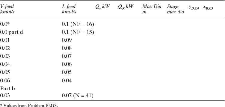
Note that QR decreases, but since energy will be required to vaporize the feed, the net change in heating requirement is negligible. The maximum diameter decreases, but the purity of the distillate and the bottoms decreases.
b. To obtain a purer product, increase N (Aspen notation) to 41, use NF,liq = 18 and NF,vap = 21. Then repeat the run with 0.03 kmol/s of vapor feed and 0.07 kmol/s of liquid feed. Compare with the all-liquid feed run. How much volume decrease is there in the column?
c. Do a tray-rating run with the diameter calculated in part b, and use defaults for tray spacing and for the downcomer. Record the maximum downcomer backup and the tray at which it occurs and the maximum weir loading and the tray at which it occurs.
d. Since Problem 10.G3 has not been optimized, try feed of the liquid on stage 15 with no vapor feed. Record the maximum downcomer backup and the tray at which it occurs and the maximum weir loading and the tray at which it occurs.
G5. 300.0 kmol/h of a saturated liquid feed that is 40.0 mol% n-nonane (C9) and 60.0 mol% n-decane (C10) at 11.0 kPa is fed to a distillation column with N = 30 (including a total condenser and a kettle-type reboiler). Feed is at Nfeed = 15, D = 120.0 kmol/h and L/D = 2.0. Use Peng-Robinson correlation. For both parts a and b find the distillate and bottoms mole fractions, the fraction of vapor in the feed flashing in the column, the required diameter of the column and tray with the largest diameter (sieve trays at 80% of flood with Fair flooding correlation and defaults for the other terms), the distillate and bottoms temperatures in K, QC and QR in kW, and the pressure in the top and bottom of the column in kPa.
a. Set the pressure of the condenser at 10.0 kPa, and make the pressure of the column constant.
b. Set the pressure of the condenser at 10.0 kPa, and set a pressure drop per stage and pressure drop in the condenser at 6.0 mm of water.
Chapter 10 Appendix. Tray and Downcomer Design with Computer Simulator
This appendix shows how the Aspen Plus simulator can be used to do detailed tray and downcomer design.
Lab 10. Detailed Design
Preparation:
• Review computer labs as needed.
• Read the details of tray and downcomer design in this chapter.
Goal: Use Aspen Plus simulation to explore detailed design of trays and downcomers.
Aspen Plus uses RadFrac’s Tray Rating option to do detailed tray and downcomer design.
I. Problem Setup. Set up and run the following distillation in Aspen Plus.
1. We wish to distil a feed of 1.0 kmol/s of a feed at 25.0°C and 15.0 atm. The feed is 10.0 mol% ethane, 30.0 mol% propane, 50.0 mol% n-butane, and 10.0 mol% n-pentane. Use the Peng-Robinson VLE correlation. Design a column with N = 35 (Aspen notation) and the feed on stage 16. The column operates at 15.0 atm, has a partial condenser, and produces a vapor distillate with D = 0.400 kmol/s. A kettle-type reboiler is used. Reflux ratio is L/D = 2.5.* Once your results look reasonable, continue with part II.
* This problem was adapted from Example 14.3.1 in R. Taylor and R. Krishna, Multicomponent Mass Transfer, Wiley, New York, 1993.
II. Tray Sizing and Rating options.
2. In the All Items list in the block for your distillation column, click Tray Sizing. In the Object Manager, click New, and call this section 1. Section 1 is stages 2 to 15. In both sections use sieve plates with the Fair flooding calculation method with flooding at 70%. For other variables initially use the default numbers for the variables in both sections. Once you have completed tray-sizing section 1, click Tray Sizing again, and in the Object Manager, click New, and call this section 2. Section 2 is stages 16 to 34.
3. Click Next, run the simulation, and look at the reports for both Streams and Blocks. Is the feed a liquid, a vapor, or a two-phase system? Which components are the light and heavy keys? Note that the two sections have different diameters. Which section has a larger diameter? Why? If the column were designed with a single section, it would all have to be the larger diameter.
Note: the methods in Section 10.4 might allow design of a column with a constant diameter between the two calculated values.
4. Now click Tray Rating. In the Object Manager, Click New, and call this section 1 (trays 2 to 15). Input the same information for section 1 as you did for section 1 in Tray Sizing. Use the same maximum diameter on trays 2 to 15 as you obtained previously for section 1 from the tray sizing routine. Use a weir height of 0.050 m. On the Design/Pdrop tab, pick the Fair flooding calculation method, and do NOT check Update section pressure drop. In the Layout tab the tray type is sieve, and use the defaults for the other items. At this point do not put any numbers into the Downcomers tab (this means default values will be used). Return to Tray Rating Object Manager, click New, and call it section 2 (trays 16 to 34). Put in the same values as for section 1, except use the maximum diameter that was calculated by tray sizing for section 2.
5. Click Next, run the simulation, and look at the report for the column. Note that the report now contains a Tray Rating section after the Tray Sizing section. Look at the flooding factors for both sections. Why are the maximum values of the flooding factor = 0.70 in both sections?
A. Look at the downcomer (DC) backup for both sections. Section 1 should be okay (backup < tray spacing), but section 2 is not okay. Section 2 would flood due to excessive downcomer backup and will not operate. (The flooding calculation done in tray sizing is for entrainment flooding—that calculation does not consider flooding caused by downcomer backup.)
B. Another concern is whether the weir can handle all of the liquid going over it. Think of the weir as a dam on a river. As the water flow rate goes up, the height above the weir increases. A rule of thumb for design (Torzewski, 2009) is that the maximum weir loading is (70 m3 of liquid/h)/(m weir length) = 0.01944 m2/s = 194.4 cm2/s. Both sections have weir loadings (listed under Rating Results) that are too high.
6. We must adjust section 2 so that the downcomer does not backup excessively. This can be done by increasing the size of the downcomer and/or increasing the tray spacing and/or adding additional flow passes. We must also reduce the weir loadings in both sections. This can be done by adding additional passes. Since additional passes attack both problems, we will do this first. Increase both sections 1 and 2 to two passes. Use default values for other variables that were not previously set. Run the program, and look at the downcomer backup, the fraction flooding, and the weir loading. Section 1 should be okay on the downcomer backup and weir loading, but the fraction flooding is slightly too high. In section 2 the weir loading is still too high, and fraction flooding is greater than the design condition.
7. Increase section 2 to four passes, and run the simulation again. Look at the downcomer backup, the fraction flooding, and the weir loading. The weir loading is still a bit too high, and the fractional flooding is higher than the design condition.
8. Adjust the diameter of the column in sections 1 and 2 to return to 70% flooding. Since the fraction of flooding is directly proportional to the column area [proportional to (diameter)2], we can calculate the new diameter needed from
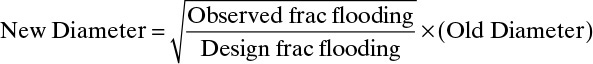
Run the simulation, and look at the tray-rating results. Fractional flooding should now be essentially the desired 0.7, and since the increase in diameter decreases weir loadings, they should both be less than the limiting weir loading.
9. Now we need to look at a number of other aspects based on rules of thumb for design (Torzewski, 2009).
A. For column diameter > 3.0 m, we need tray spacing > 0.6 m. This is okay.
B. The downcomer clearance < weir height. This is okay.
10. Report the distillate (remember it is a vapor) and bottoms mole fractions, the diameters and largest percentages of flooding, the largest fractional downcomer backups, and the weir loadings in both sections 1 and 2.
Result: The resulting design is satisfactory. Accept this as an initial design. Note that this column is not optimized but is a workable design.
III. Changes in Operating Conditions.
11. Turndown. Assume the column designed in step 8 has been built. Because of slow sales, the feed rate is reduced to 0.75 kmol/s. Change F and D, and rerun the simulation. Then check both tray ratings to see if there are problems.
Note: The low fraction of flooding could cause weeping problems. Properly functioning valve trays would be better than sieve trays.
12. Increased Feed Rate. Assume the column designed in step 8 has been built. Because of high sales, the company wants to increase the feed rate as much as possible.
12A. Assume that an increase of the flooding to 90% is acceptable. (Since the Fair design procedure is known to be conservative, although 90% of flood is high, the column will probably operate satisfactorily as long as there is good control of the feed rate. Use of 90% with other design procedures could be problematic.) Estimate the new feed rate as
Fnew = Fold × [(new % flood)/(old % flood)]
Change F and D, and rerun the simulation. If you change D appropriately, you should get the same separation. Then check both tray ratings to see what problems occur.
12B. Since the previous method gives weir loadings that are too high, a more conservative increase can be obtained by estimating the new feed rate from the acceptable weir loading.
Fnew = Fdesign × [(new weir loading)/(old weir loading at design flood rate)]
The new weir loading is the maximum allowable value of 194.4 cm2/s mentioned in step 5B. Calculate a new flow rate from the weir loadings of both sections of the column, and use the lower value. Adjust the distillate flow rate for the new feed rate. Run the simulation. Which section controls the feed rate when calculated this way? Check the distillate and bottoms mole fractions, the largest percentages of flooding, the largest fractional downcomer backups, and the weir loadings in both sections 1 and 2. Although flooding is > 70%, this design should operate properly with the increased feed rate. Report your new feed rate.
Note: Stage efficiency may well be reduced for both turndown and increased feed rate, but equilibrium-based calculations done by Aspen Plus do not correct for this.