
Chapter 4. Binary Column Distillation: Internal Stage-by-Stage Balances
4.0 Summary—Objectives
In this long chapter we develop the stage-by-stage balances for distillation columns and show how to solve these equations when molar flow rates in each section of the column are constant (called constant molal overflow [CMO]). When finished studying this chapter, you should be able to satisfy the following objectives:
1. Write mass and energy balances and equilibrium expressions for any stage in a column
2. Explain what CMO is, and determine if CMO is valid in a given situation
3. Derive the operating equations for CMO systems
4. Calculate the feed quality, and determine its effect on flow rates. Plot the feed line on a y-x diagram
5. Determine the number of stages required using the Lewis method and the McCabe-Thiele method
6. Develop and explain composition, temperature, and flow profiles
7. Solve any binary distillation problem where CMO is valid. This includes:
a. Open steam
b. Multiple feeds
c. Partial condensers and total reboilers
d. Side streams
e. Intermediate reboilers and condensers
f. Stripping and enriching columns
g. Total and minimum reflux
h. Overall and Murphree efficiencies
i. Simulation problems
j. Any combination of the above
8. Include the effects of subcooled reflux or superheated boilup
9. Use a computer process simulator for simulation of binary distillation
4.1 Internal Balances
In Chapter 3 we introduced column distillation and developed the external balance equations. In this chapter we look inside the column. The number of equilibrium stages required for the separation can be determined by solving mass and energy balances and equilibrium in a stage-by-stage fashion. We start at the top of the column and write the balances and equilibrium relationship for the first stage and then, once we have determined the unknown variables for the first stage, we write balances for the second stage. Utilizing the variables just calculated we can again calculate the unknowns. We can now proceed down the column in this stage-by-stage fashion until we reach the bottom. We could also start at the bottom and proceed upward. Methods for nonequilibrium stages are discussed in Section 4.11.
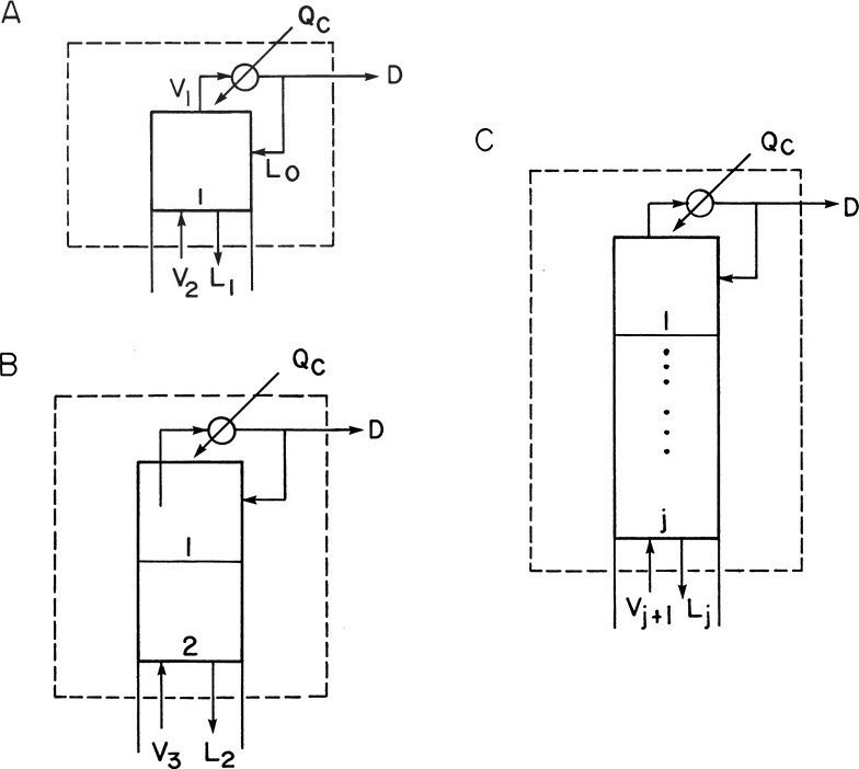
In the enriching section of the column it is convenient to use a balance envelope, as shown in Figure 4-1, that goes around the desired stage and around the condenser. The balance envelope for the first stage is shown in Figure 4-1A. The overall mass balance is
The more volatile component (MVC) mass balance is
For a well-insulated, adiabatic column (Qcolumn = 0), the energy balance is
Assuming that each stage is an equilibrium stage, liquid and vapor leaving each stage are in equilibrium. For a binary system, Gibbs phase rule is
Degrees of freedom = C – P + 2 = 2 – 2 + 2 = 2
Since pressure has been set, there is one remaining degree of freedom. Thus the intensive variables are all functions of a single variable. For the saturated liquid we can write
and for the saturated vapor,
The liquid and vapor mole fractions leaving a stage are also related:
Equations (4-4) for stage 1 represent the equilibrium relationship. Their exact form depends on the chemical system being separated. For example, we found that Eq. (2.B-2), a sixth-order polynomial, was a reasonable fit to the equilibrium data for Eq. (4-4c) for ethanol-water equilibrium. Equations (4-1, stage 1) to (4-4c, stage 1) are six equations with six unknowns: L1, V2, x1, y2, H2, and h1.
Since we have six equations and six unknowns, in theory, we can solve for the six unknowns. The exact methods for calculating the unknowns are the subject of the remainder of this chapter. For now we will just note that we can solve for the unknowns and then proceed to the second stage. For the second stage we will use the balance envelope shown in Figure 4-1B. The mass balances are now
while the energy balance is
The equilibrium relationships are
Again we have six equations with six unknowns. The unknowns are now L2, V3, x2, y3, H3, and h2.
We can now proceed to the third stage and utilize the same procedures. After that, we can go to the fourth stage and then the fifth stage and so forth. For a general stage j (j can be from 1 to f – 1, where f is the feed stage) in the enriching section, the balance envelope is shown in Figure 4-1C. For this stage the mass and energy balances are
and
while the equilibrium relationships are
When we reach stage j the values of yj, Qc, D, and hD will be known, and the unknown variables will be Lj, Vj+1, xj, yj+1, Hj+1, and hj. At the feed stage the mass and energy balances will change because of the addition of the feed stream.
Before continuing, note the symmetry of the mass and energy balances and the equilibrium relationships as we go from stage to stage. Equations (4-1) for stages 1, 2, and j all have the same structure and differ only in subscripts. Equations (4-1, stage 1) and (4-1, stage 2) can be obtained from the general Eq. (4-1, stage j) by replacing j with 1 or 2, respectively. The same observations can be made for the other equations. The unknown variables as we go from stage to stage are also similar and differ only in subscript.
In addition to this symmetry from stage to stage, there is symmetry between equations for the same stage. Thus Eqs. (4-1, stage j), (4-2, stage j), and (4-3, stage j) are all steady-state balances that state input = output. In all three equations the output (of overall mass, solute, or energy) is associated with streams Lj and D. The input is associated with stream Vj+1 and for energy with the cooling load, Qc.
Below the feed stage the balance equations must change, but the equilibrium relationships in Eqs. (4-4a, b, and c) will be unchanged. The balance envelopes in the stripping section are shown in Figure 4-2 for a column with a partial reboiler. The bars over the flow rates signify that they are in the stripping section. It is traditional and simplest to write the stripping section balances around the bottom of the column using the balance envelope shown in Figure 4-2. Then these balances around stage f + 1 (immediately below the feed plate) are
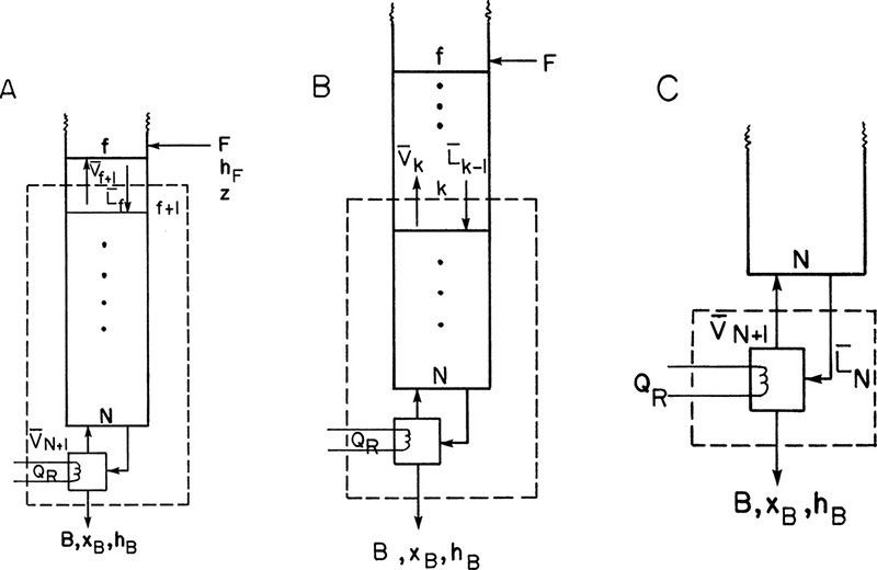
FIGURE 4-2. Stripping section balance envelopes; (A) below feed stage (stage f + 1), (B) stage k, (C) partial reboiler
The equilibrium relationships are Eqs. (4-4) written for stage f + 1:
These six equations have six unknowns: ![]() ,
, ![]() , xf, yf+1, Hf+1, and hf. xB is specified in the problem statement; B and QR were calculated from the column balances; and yf (required for the last equation) was obtained from the solution of Eqs. (4-1, stage j) to (4-4c, stage j) with j = f – 1. At the feed stage we change from one set of balance envelopes to another.
, xf, yf+1, Hf+1, and hf. xB is specified in the problem statement; B and QR were calculated from the column balances; and yf (required for the last equation) was obtained from the solution of Eqs. (4-1, stage j) to (4-4c, stage j) with j = f – 1. At the feed stage we change from one set of balance envelopes to another.
Note that the same equations will be obtained if we write the balances above stage f + 1 and around the top of the distillation column (use a different balance envelope). This is easily illustrated with the overall mass balance, which becomes
Rearranging, we have
However, since the external column mass balance says F – D = B, the last equation becomes
which is Eq. (4-5, stage f + 1). Similar results are obtained for the other balance equations. Thus the balance envelope we use is arbitrary.
Once the six equations, Eqs. (4-4a) to (4-7), for stage f + 1 have been solved, we can proceed down the column to the next stage, f + 2. For a balance envelope around general stage k, as shown in Figure 4-2B, the equations are
The equilibrium expression will correspond to Eqs. (4-4, stage f + 1), with k – 1 replacing f as a subscript. Thus
A partial reboiler, as shown in Figure 4-2C, acts as an equilibrium contact. If we consider the reboiler as stage N + 1, the balances for the envelope shown in Figure 4-2C can be obtained by setting k = N + 1 and k – 1 = N in Eqs. (4-5, stage k), (4-6, stage k), and (4-7, stage k).
If xN+1 = xB, the N + 1 equilibrium contacts give us exactly the specified separation, and the problem is finished. If xN+1 < xB while xN > xB, the N + 1 equilibrium contacts give slightly more separation than is required.
Just as the balance equations in the enriching section are symmetric from stage to stage, they are also symmetric in the stripping section.
4.2 Binary Stage-by-Stage Solution Methods
The challenge for any stage-by-stage solution method is to solve the three balance equations and the three equilibrium relationships simultaneously in an efficient manner. This problem was first solved by Sorel (1893), and graphical solutions of Sorel’s method were developed independently by Ponchon (1921) and Savarit (1922). (Kockmann [2014] covers the history of distillation.) These methods all solve the complete mass and energy balance and equilibrium relationships stage by stage. Starting at the top of the column, as shown in Figure 4-1A, we can find the liquid composition, x1, in equilibrium with the leaving vapor composition, y1, from Eq. (4-4c, stage 1). The liquid enthalpy, h1, is found from Eqs. (4-4a, stage 1). The remaining four equations, Eqs. (4-1) to (4-3) and (4-4b), for stage 1 are coupled and must be solved simultaneously. The Ponchon-Savarit method does this graphically. The Sorel method uses a trial-and-error procedure on each stage.
The trial-and-error calculations on every stage of the Sorel method are obviously slow and laborious. Lewis (1922) noted that in many cases the molar vapor and liquid flow rates in each section (a region between input and output ports) were constant. Thus in Figures 4-1 and 4-2
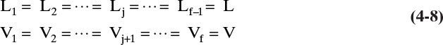
and

For each additional column section there will be another set of equations for constant flow rates. Note that in general ![]() and
and ![]() . Equations (4-8) and (4-9) are valid if every time a mole of vapor is condensed, a mole of liquid is vaporized. This occurs under the following conditions:
. Equations (4-8) and (4-9) are valid if every time a mole of vapor is condensed, a mole of liquid is vaporized. This occurs under the following conditions:
1. The heat of vaporization per mole λ is constant; that is, λ does not depend on concentration. This condition is the most important criterion.
2. The specific heat changes are small compared to latent heat changes.
3. The column is adiabatic.
Lewis called this set of conditions CMO. An alternative to conditions 1 and 2 is
4. The saturated liquid and vapor lines on an enthalpy-composition diagram (in molar units) are parallel.
For some systems, such as hydrocarbons, the latent heat of vaporization per kilogram is approximately constant. In such situations the mass flow rates are constant, and constant mass overflow should be used.
The Lewis method assumes before the calculation is done that CMO is valid. Thus Eqs. (4-8) and (4-9) are valid. With this assumption, the energy balance, Eqs. (4-3) and (4-7), will be automatically satisfied. Then only Eqs. (4-1), (4-2), and (4-4c) or Eqs. (4-5), (4-6), and (4-4c) need be solved. Equations (4-1, stage j) and (4-2, stage j) can be combined:
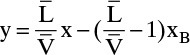
Solving for yj+1, we have
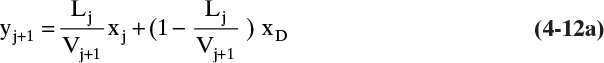
Since L and V are constant, this equation becomes
Equation (4-12b) is the operating equation in the enriching section. It relates the concentrations of two passing streams in the column and thus represents the mass balances in the enriching section. Equation (4-12b) is solved sequentially with the equilibrium expression for xj, Eq. (4-4c, stage j).
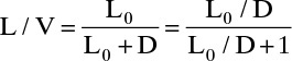
To start, we first use the external column balances to calculate D and B. Then
In the stripping section Eqs. (4-5, stage k) and (4-6, stage k) are combined to give

With CMO, ![]() and
and ![]() are constant, and the resulting stripping section operating equation is
are constant, and the resulting stripping section operating equation is
Once we know ![]() we can calculate by alternating between the operating Eq. (4-14b) and equilibrium Eq. (4-4c, stage k).
we can calculate by alternating between the operating Eq. (4-14b) and equilibrium Eq. (4-4c, stage k).
The phase and temperature of the feed affects the vapor and liquid flow rates in the column. For instance, if the feed is liquid, the liquid flow rate below the feed stage must be greater than liquid flow above the feed stage, ![]() , and if the feed is a vapor,
, and if the feed is a vapor, ![]() . These effects can be quantified by writing mass and energy balances around the feed stage. The feed stage is shown schematically in Figure 4-3. The overall mass balance and the energy balance for the balance envelope shown in Figure 4-3 are
. These effects can be quantified by writing mass and energy balances around the feed stage. The feed stage is shown schematically in Figure 4-3. The overall mass balance and the energy balance for the balance envelope shown in Figure 4-3 are
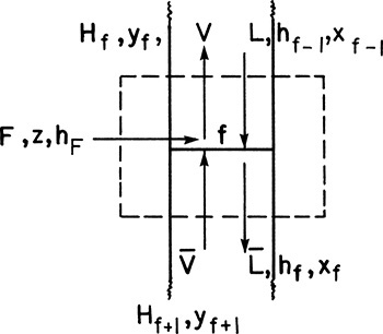
and
(Despite the use of “hF” as the symbol for the feed enthalpy, the feed can be a liquid or vapor or a two-phase mixture.) If we assume CMO, neither the vapor enthalpies nor the liquid enthalpies vary much from stage to stage. Thus Hf+1 ∼ Hf and hf–1 ∼ hf. Then Eq. (4-16) becomes
The mass balance Eq. (4-15) can be conveniently solved for ![]() :
:
which can be substituted into the energy balance to give us
or
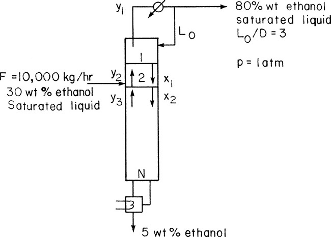
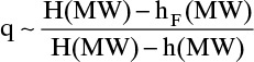
The “quality” q can be generalized to


The value of q can be approximated from

This result is analogous to the use of q in flash distillation. Since the liquid and vapor enthalpies can be estimated, we can calculate q from Eq. (4-17). Then
The quality q is the fraction of feed that is liquid. For example, if the feed is a saturated liquid, hF = h, q = 1, and ![]() . Once
. Once ![]() has been determined,
has been determined, ![]() is calculated from either Eq. (4-15) or Eq. (4-5, stage f + 1) or from
is calculated from either Eq. (4-15) or Eq. (4-5, stage f + 1) or from
This equation can be derived from Eqs. (4-15) and (4-19a).
When the feed is a two-phase mixture, we can analyze the feed in exactly the same way as we analyzed flash distillation. If f is the fraction of feed that is vapor, then

In words this is

and we can estimate the fraction vapor from

If CMO is valid, the vapor and liquid flow rates in the column sections above and below the feed are related by
EXAMPLE 4-1. Stage-by-stage calculations by the Lewis method
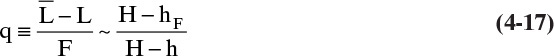
A steady-state countercurrent, staged distillation column is separating ethanol from water. The feed is a 30.0 wt% ethanol, 70.0 wt% water mixture that is a saturated liquid at 1 atm pressure. Flow rate of feed is 10,000 kg/h. The column operates at a pressure of 1 atm. The reflux is returned as a saturated liquid. A reflux ratio of L/D = 3.0 is being used. Bottoms composition is xB = 0.05 (weight fraction ethanol), and distillate composition is xD = 0.80 (weight fraction ethanol). The system has a total condenser and a partial reboiler. The column is well insulated. Use the Lewis method to find the number of equilibrium contacts required if the feed is input on the second stage from the top.
Solution
A. Define. The column and known information are shown in the following figure. Find the number of equilibrium contacts required.
B. Explore. This problem is very similar to Example 3-1. The solutions for B and D obtained in that example are still correct: B = 6667 kg/h, and D = 3333 kg/h. Equilibrium data are available in weight fractions in Figure 2-4 and in mole fraction units in Figure 2-2 and Table 2-1. To use the Lewis method we must have CMO. We can check this by comparing the latent heat per mole of pure ethanol and pure water. (This checks the most important criterion for CMO. Since the column is well insulated, the third criterion, adiabatic, will be satisfied.) The latent heats are (Himmelblau, 1974)
λE = 9.22 kcal/mol, λW = 9.7171 kcal/mol
The difference of roughly 5% is reasonable particularly since we always use the ratio of L/V or ![]() . (Using the ratio causes some of the change in L and V to divide out.) Thus we will assume CMO. To have constant flow rates we must convert flows and compositions to molar units. MWW = 18 and MWE = 46.
. (Using the ratio causes some of the change in L and V to divide out.) Thus we will assume CMO. To have constant flow rates we must convert flows and compositions to molar units. MWW = 18 and MWE = 46.
C. Plan. After converting to molar units, do preliminary calculations to determine L/V and ![]() . Then start at the top, alternating between equilibrium [Figure 2-2 or Eq. (2.B-2)] and the top operating Eq. (4-12b). Since stage 2 is the feed stage, calculate y3 from the bottom operating Eq. (4-14).
. Then start at the top, alternating between equilibrium [Figure 2-2 or Eq. (2.B-2)] and the top operating Eq. (4-12b). Since stage 2 is the feed stage, calculate y3 from the bottom operating Eq. (4-14).
Preliminary Calculations: To convert to molar units choose a convenient basis, such as 1.0 kg of feed.
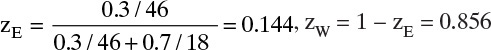
Average molecular weight of feed is
Feed rate = (10,000 kg/h)/(22.03 kg/kmol) = 453.9 kmol/h. Distillate mole fraction,
For distillate, the average molecular weight is
This is also the average for the reflux liquid and vapor stream V since they are all the same composition. Then D = (3333 kg/h)/35.08 = 95.23 kmol/h and L = (L/D)D = 3(95.23) = 285.7 kmol/h, and V = L + D = 380.9 kmol/h. Thus L/V = 285.7/380.9 = 0.75. Because of CMO, L/V is constant in the rectifying section.
Since the feed is a saturated liquid,
Since a saturated liquid feed does not affect the vapor, ![]() . Thus
. Thus ![]() . An internal check on consistency is L/V < 1 and
. An internal check on consistency is L/V < 1 and ![]() .
.
Stage-by-Stage Calculations: At the top of the column, y1 = xD = 0.61 (mole fraction). Liquid stream L1 of concentration x1 is in equilibrium with the vapor stream y1. From Figure 2-2, x1 = 0.4. (Note that y1 > x1, since ethanol is the more volatile component.) Vapor stream y2 is a passing stream relative to x1 and can be determined from the operating Eq. (4-12).
Stream x2 is in equilibrium with y2. From Figure 2-2 we obtain x2 = 0.11. Since stage 2 is the feed stage, use bottom operating Eq. (4-14) for y3.

Stream x3 is in equilibrium with y3. From Figure 2-2, this is x3 = 0.02. Since x3 = xB (in mole fraction), we are finished.
The third equilibrium contact is the partial reboiler. Thus the column has two equilibrium stages in addition to the partial reboiler.
E. Check. This is a small number of stages. However, not much separation is required, the external reflux ratio is large, and the separation of ethanol from water is easy in this concentration range. Thus the answer is reasonable. We can check the calculation of L/V with mass balances.
Since V1 = L0 + D,
Since L0, V1, and D are the same composition, L0/D and L0/V1 have the same values in mass and molar units. We can check the equilibrium calculation with Eq. (2.B-2). For example, for y1 = 0.61 we obtain x1 = 0.385.
F. Generalizations. Always check that CMO is valid, and then convert all flows and compositions into molar units. The procedure for stepping off stages is easily programmed on a spreadsheet (see Appendix B of this chapter). We could also have started at the bottom and worked our way up the column stage by stage. Going up the column we calculate y values from equilibrium and x values from the operating equations.
Note that L/V < 1 and ![]() . This relationship makes sense, since we must have a net flow of material upward in the rectifying section to obtain a distillate product and a net flow downward in the stripping section to obtain a bottoms product. We must also have a net upward flow of ethanol in the rectifying section (Lxj < Vyj+1) and in the stripping section
. This relationship makes sense, since we must have a net flow of material upward in the rectifying section to obtain a distillate product and a net flow downward in the stripping section to obtain a bottoms product. We must also have a net upward flow of ethanol in the rectifying section (Lxj < Vyj+1) and in the stripping section ![]() . These conditions are satisfied by all pairs of passing streams.
. These conditions are satisfied by all pairs of passing streams.
The Lewis method is obviously much faster and more convenient than the Sorel method. It is also easier to program on a computer or in a spreadsheet. In addition, it is easier to understand the physical reasons why separation occurs instead of becoming lost in the algebraic details. However, remember that the Lewis method is based on the assumption of CMO. If CMO is not valid, then the answers will be incorrect.
If you find the Lewis method is confusing, continue to the next section. The graphical McCabe-Thiele procedure explained in Section 4.3 is easier for many students to understand. After completing the McCabe-Thiele procedure, return to this section and study the Lewis method again.
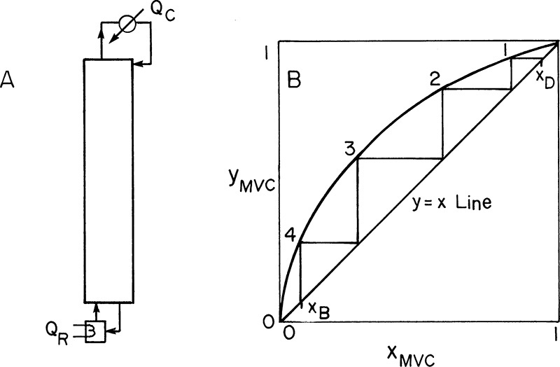
4.3 Introduction to the McCabe-Thiele Method
McCabe and Thiele (1925) developed a graphical solution method based on Lewis’ method and the observation that the operating Eqs. (4-12b) and (4-14) plot as straight lines (the operating lines) on a y-x diagram. On this graph the equilibrium relationship can be solved from the y-x equilibrium curve and the mass balances from the operating lines.
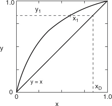
To illustrate, consider a typical design problem for a binary distillation column such as the one illustrated in Figure 3-8. Assume that equilibrium data are available at the operating pressure of the column. These data are plotted in Figure 4-4. At the top of the column is a total condenser. As noted in Chapter 3 in Eq. (3-10a), this condition means that y1 = xD = x0. The vapor leaving the first stage is in equilibrium with the liquid leaving the first stage. This liquid composition, x1, can be determined from the equilibrium curve at y = y1. This is illustrated in Figure 4-4.
Liquid stream L1 of composition x1 passes vapor stream V2 of composition y2 inside the column (Figures 3-8 and 4-1A). When the mass balances are written around stage 1 and the top of the column (see balance envelope in Figure 4-1A), the result after assuming CMO and doing some algebraic manipulations is Eq. (4-12) with j = 1. This equation can be plotted as a straight line on the y-x diagram. Suppressing subscripts j + 1 and j, we write Eq. (4-12b) as
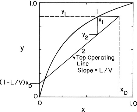
which is understood to apply to passing streams. Eq. (4-23) plots as a straight line (the top operating line) with a slope of L/V and a y intercept (x = 0) of (1 – L/V)xD. Once Eq. (4-23) has been plotted, y2 is easily found from the y value at x = x1. This is illustrated in Figure 4-5. Note that the top operating line goes through the point (y1, xD) since these coordinates satisfy Eq. (4-23).
With y2 known we can proceed down the column. Since x2 and y2 are in equilibrium, we obtain x2 from the equilibrium curve. Then we obtain y3 from the operating line (mass balances), since x2 and y3 are the compositions of passing streams. This procedure of stepping off stages is shown in Figure 4-6. It can be continued as long as we are in the rectifying section. Note that this procedure produces a staircase on the y-x, or McCabe-Thiele, diagram. Instead of memorizing this procedure, you should follow the points on the diagram and compare them to the schematics of a distillation column (Figures 3-8 and 4-1). Note that the horizontal and vertical lines have no physical meaning. The points on the equilibrium curve (squares in Figure 4-6) represent liquid and vapor streams leaving an equilibrium stage. The points on the operating line (circles in Figure 4-6) represent the liquid and vapor streams passing each other in the column.
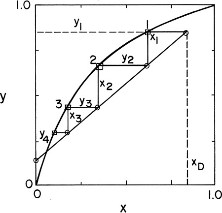
In the stripping section Eq. (4-23) is no longer valid since different mass balances and, hence, a different operating equation are required. The stripping section operating equation was given in Eq. (4-14b). When subscripts k and k – 1 are suppressed this equation becomes
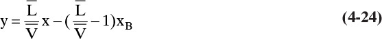
Equation (4-24) plots as a straight line with slope ![]() and y intercept
and y intercept ![]() , as shown in Figure 4-7. This bottom operating line applies to passing streams in the stripping section. Liquid leaving the partial reboiler has a mole fraction of xB = xN+1. We know that the vapor leaving the partial reboiler (composition yN+1) is in equilibrium with xB, and we can find yN+1 from the equilibrium curve. Since liquid of composition xN is a passing stream to vapor of composition yN+1 (compare Figures 4-2 and 4-7), xN is found from the bottom operating line. This process of stepping off stages by alternating between the equilibrium curve and the bottom operating line continues as long as we are in the stripping section.
, as shown in Figure 4-7. This bottom operating line applies to passing streams in the stripping section. Liquid leaving the partial reboiler has a mole fraction of xB = xN+1. We know that the vapor leaving the partial reboiler (composition yN+1) is in equilibrium with xB, and we can find yN+1 from the equilibrium curve. Since liquid of composition xN is a passing stream to vapor of composition yN+1 (compare Figures 4-2 and 4-7), xN is found from the bottom operating line. This process of stepping off stages by alternating between the equilibrium curve and the bottom operating line continues as long as we are in the stripping section.
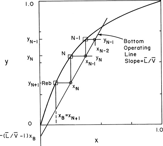
If we are stepping off stages down the column, at the feed stage f we switch from the top operating line to the bottom operating line (refer to Figure 4-3, a schematic of the feed stage). Above the feed stage we calculate yf from the top operating line. Since liquid and vapor leaving the feed stage are assumed to be in equilibrium, we can determine xf from the equilibrium curve at y = yf and then find yf+1 from the bottom operating line. This procedure is illustrated in Figure 4-8A, in which stage 3 is the feed stage. The separation shown in Figure 4-8A would require 5 equilibrium stages plus an equilibrium partial reboiler, or six equilibrium contacts, when stage 3 is used as the feed stage. In this problem, stage 3 is the optimum feed stage. That is, a separation will require the fewest total number of stages when stage 3 is the feed stage. Note in Figures 4-8B and 4-8C that if stage 2 or stage 5 is used, more total stages are required. For binary distillation the optimum feed plate is easy to determine; it is always the stage in which the step in the staircase includes the point of intersection of the two operating lines (compare Figure 4-8A to Figures 4-8B and 4-8C). A mathematical analysis of the optimum feed plate location suitable for computer calculation with the Lewis method is developed later.
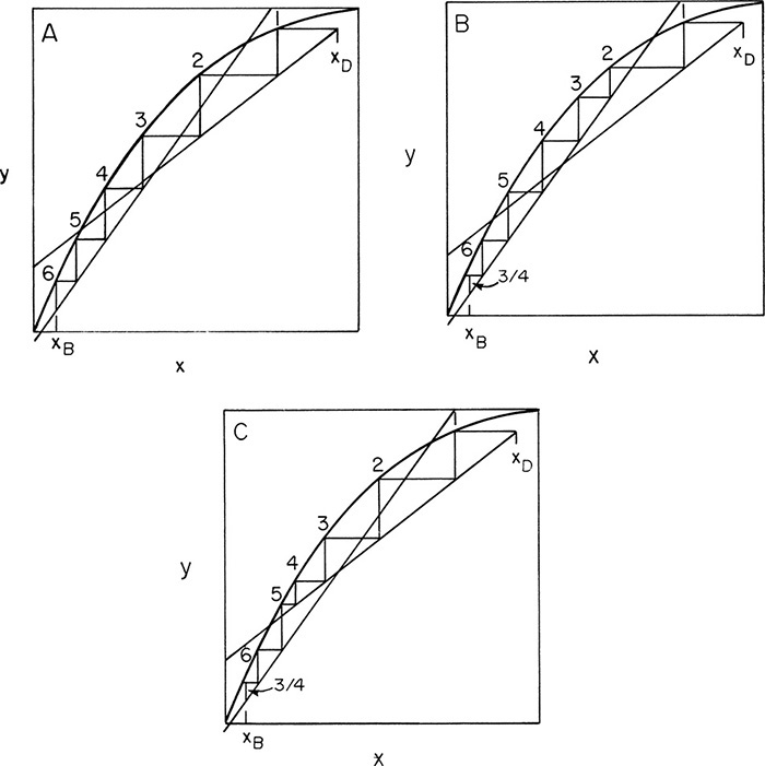
FIGURE 4-8. McCabe-Thiele diagram for entire column; (A) optimum feed stage (stage 3); (B) feed stage too high (stage 2); (C) feed stage too low (stage 5)
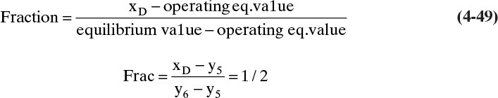
When stepping off stages from the top down, a fractional number of stages can be calculated as (see Figures 4-8B and 4-8C)

where the distances are measured horizontally on the diagram. The fraction has no physical meaning because we build either five or six stages; however, the fraction is somewhat useful when the stage efficiency is << 1.
Now that we know how to perform the stage-by-stage calculations on a McCabe-Thiele diagram, let us consider how to start with the design problem given in Figure 3-8 and Tables 3-1 and 3-2. The known variables are F, z, q, xD, xB, L0/D, p, and saturated liquid reflux, and we use the optimum feed location. Since the reflux is a saturated liquid, there will be no change in flow rates on stage 1 and L0 = L1 and V1 = V2. This allows us to calculate the internal reflux ratio, L/V, from the external reflux ratio, L0/D, which is specified.
With L/V and xD known, the top operating Eq. (4-23) is fully specified and can be plotted as a straight line.
Since the boilup ratio, ![]() , is not specified, we cannot directly calculate
, is not specified, we cannot directly calculate ![]() , the slope of the bottom operating line. Instead, we need to utilize the condition of the feed to determine flow rates in the stripping section. The same procedure used with the Lewis method can be used here. The feed quality, q, is calculated from Eq. (4-17). Then
, the slope of the bottom operating line. Instead, we need to utilize the condition of the feed to determine flow rates in the stripping section. The same procedure used with the Lewis method can be used here. The feed quality, q, is calculated from Eq. (4-17). Then ![]() is given by Eq. (4-19a),
is given by Eq. (4-19a), ![]() , and
, and ![]() . We can calculate L as (L/D)D, where D and B are found from mass balances around the entire column. With
. We can calculate L as (L/D)D, where D and B are found from mass balances around the entire column. With ![]() and xB known, the bottom operating equation is fully specified, and the bottom operating line can be plotted.
and xB known, the bottom operating equation is fully specified, and the bottom operating line can be plotted.
4.4 Feed Line
In any section of the column between feeds and/or product streams the mass balances are represented by an operating line that can be derived by drawing a mass balance envelope through an arbitrary stage in the section and around the top or bottom of the column. When material is added or withdrawn from the column the mass balances and the operating lines change. In the previous section the effect of a feed on the operating lines was determined from the feed quality and mass balances around the entire column. Here we will develop a graphical method for determining the effect of a feed on the operating lines.
Consider the simple, single-feed column with a total condenser and a partial reboiler shown in Figure 3-8. If CMO is valid the MVC mass balance in the rectifying section is
while the balance in the stripping section is
At the feed plate we switch from one mass balance to the other. We wish to find the point at which the top operating line—representing Eq. (4-27)—intersects the bottom operating line—representing Eq. (4-28). The intersection of these two lines means that
Equations (4-29) are valid only at the point of intersection or in the special case in which the lines are collinear (Section 4.10). Since the y’s and x’s are equal at the point of intersection, if we subtract Eq. (4-27) from Eq. (4-28), we obtain
From the overall mass balance around the entire column, Eq. (3-2), we know that the last term is –Fz. Then solving for y,

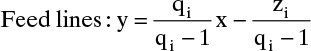
Eq. (4-30) is one form of the feed equation. Since L, ![]() , V,
, V, ![]() , F, and z are constant, it represents a straight line (the feed line) on a McCabe-Thiele diagram. Every possible intersection point of the two operating lines must occur on the feed line.
, F, and z are constant, it represents a straight line (the feed line) on a McCabe-Thiele diagram. Every possible intersection point of the two operating lines must occur on the feed line.
For the special case of a two-phase feed or one that flashes in the column to form vapor and liquid phases, we can relate Eq. (4-30) to flash distillation. In this case we have the situation shown in Figure 4-9. Part of the feed, VF, vaporizes, while the remainder is liquid, LF. Looking at the terms in Eq. (4-30), we note that ![]() is the change in liquid flow rates at the feed stage.
is the change in liquid flow rates at the feed stage.
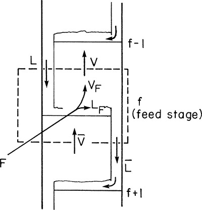
The change in vapor flow rates is
Equation (4-30) then becomes
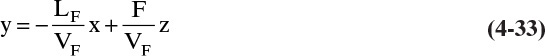
This is essentially the same as Eq. (2-11), the operating equation for flash distillation. Thus the feed line represents the flashing of the feed into the column. Equation (4-33) can also be written in terms of the fraction vaporized, f = VF/F, as [see Eqs. (2-12) and (2-13)]
In terms of the fraction remaining liquid, q = LF/F [see Eqs. (2-14) and (2-15)], Eq. (4-33) is

Eqs. (4-33) to (4-35) were derived for the special case in which the feed is a two-phase mixture, but they can be used for any type of feed. For example, if we want to derive Eq. (4-35) for the general case, we can start with Eq. (4-30). An overall mass balance around the feed stage (balance envelope shown in Figure 4-9) is
which can be rearranged to
Substituting this result into Eq. (4-30) gives
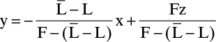
and dividing numerator and denominator of each term by the feed rate F, we get
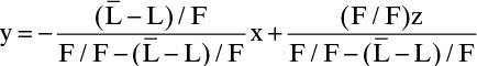
which becomes Eq. (4-35) since ![]() . Derivation of Eq. (4-34) is similar.
. Derivation of Eq. (4-34) is similar.
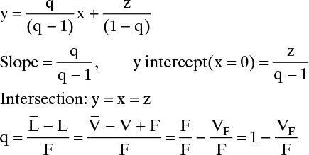
From Eq. (4-17) we can determine the value of q and hence the slope, q/(q – 1), of the feed line. For example, if the feed enters as a saturated liquid (i.e., at the liquid boiling temperature at the column pressure), then hF = h, and the numerator of Eq. (4-17) equals the denominator. Thus q = 1.0, and the slope of the feed line is q/(q – 1) = ∞. The feed line is vertical.
The various types of feeds and the slopes of the feed line are illustrated in Table 4-1 and Figure 4-10. Note that all the feed lines intersect at one point, which is at y = x. If we set y = x in Eq. (4-35), we find
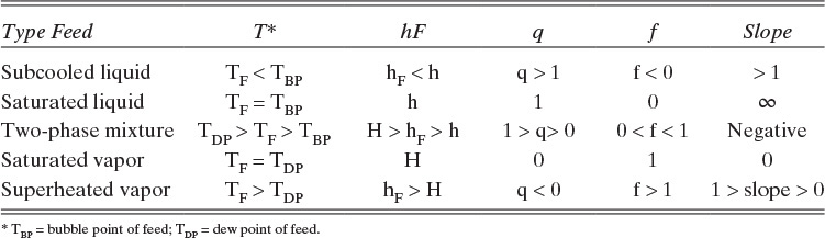
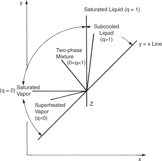
is the point of intersection (try this derivation yourself). The feed line is easy to plot from the points y = x = z or y intercept (x = 0) = z/(1 – q) or x intercept (y = 0) = z/q, and the slope, which is q/(q – 1). (The process of plotting the feed line should remind you of binary flash distillation.)
The feed line was derived from the intersection of the top and bottom operating lines. It thus represents all possible locations at which the two operating lines can intersect for a given feed (z, q). If we change the reflux ratio, we change the points of intersection, but they all lie on the feed line. This is illustrated in Figure 4-11A. If the reflux ratio is fixed (the top operating line is fixed) but q varies, the intersection point varies, as shown in Figure 4-11B. The slope of the bottom operating line, ![]() , depends on L0/D, xD, xB, and q.
, depends on L0/D, xD, xB, and q.
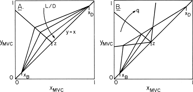
FIGURE 4-11. Operating line intersection; (A) changing reflux ratio with constant q; (B) changing q with fixed reflux ratio. Boilup ratio varies.
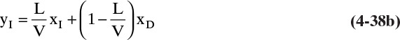
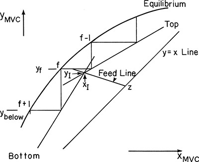
In Figure 4-8 we illustrate how to determine the optimum feed stage graphically. For computer applications an explicit test is easier to use. If the point of intersection of the two operating lines (yI, xI) is determined, then the optimum feed plate, f, is the one for which
and
This relationship is illustrated in Figure 4-12. For the simple column shown in Figure 3-8 the intersection point can be determined by straightforward but tedious algebraic manipulation as

The feed equations were developed for this simple column; however, Eqs. (4-30) and (4-33) through (4-35) are valid for any column configuration if we use the generalized definitions of q and f in Eqs (4-18a) and (4-21a).
EXAMPLE 4-2. Feed line calculations
Calculate the feed line slope for the following cases.
a. A two-phase feed where 80% of the feed is vaporized under column conditions.
Solution
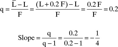
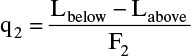
The slope is q/(q – 1), where q = (Lbelow feed – Labove feed)/F (other expressions could also be used). With a two-phase feed we have the situation shown in the figure.
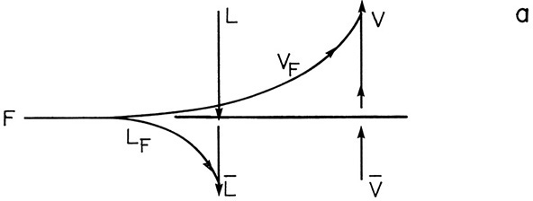
![]() . Since 80% of the feed is vapor, 20% is liquid and LF = 0.2F. Then
. Since 80% of the feed is vapor, 20% is liquid and LF = 0.2F. Then
This agrees with Figure 4-10.
b. A superheated vapor feed where 1 mole of liquid vaporizes on the feed stage for each 9 moles of feed input.
Solution
This situation is shown in the following figure.
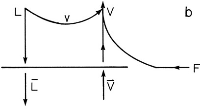
When the feed enters some liquid must be boiled to cool the feed. Thus
and the amount vaporized is v = (1/9) F. Thus
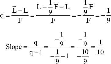
which agrees with Figure 4-10.
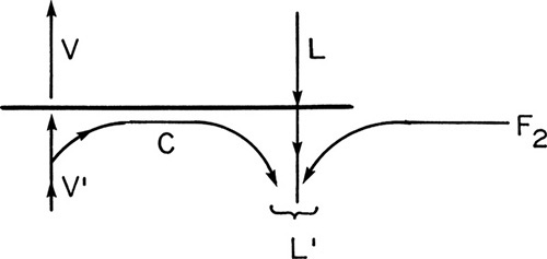
c. A liquid feed subcooled by 35°F. Average liquid heat capacity is 30 Btu/lbmol°F and λ = 15,000 Btu/lbmol.
Solution
Here some vapor must be condensed by the entering feed. Thus the situation can be depicted as shown.
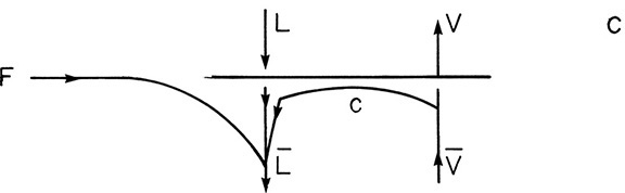
and
where c is the amount condensed. Since the column is insulated, the source of energy to heat the feed to its boiling point is the condensing vapor.

Since ΔT = TBP – TF = 35°
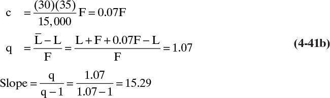
This agrees with Figure 4-10. Despite the large amount of subcooling, the feed line is fairly close to vertical, and the results will be similar to a saturated liquid feed. If TF is given instead of ΔT, we need to estimate TBP. This estimation can be done with a temperature composition graph (Figure 2-3), an enthalpy-composition graph (Figure 2-4), or a bubble-point calculation (Section 5.3).
d. Feed is 40.0 mol% ethanol – 60.0 mol% water at 40°C. Pressure is 1.0 kg/cm2.
We can now use Eq. (4-17):
The enthalpy data are available in Figure 2-4. To use that figure we must convert mole fraction to weight fraction: 40 mol% is 63 wt%. Then from Figure 2-4, hF(0.63, 40°C) = 20 kcal/kg. The vapor (represented by H) and liquid (represented by h) will be in equilibrium at the feed stage, but the concentrations of the feed stage are unknown. Comparing the feed stage locations in Figures 4-8A, 4-8B, and 4-8C, we see that liquid and vapor concentrations on the feed stage can be very different and are usually not equal to the feed concentration z. However, when CMO is valid, liquid and vapor enthalpies per mole are constant. We can calculate all enthalpies at a weight fraction of 0.63 (mole fraction = 0.40), convert the enthalpies to kcal/kmol, and estimate q. From Figure 2-4, H (0.63, saturated vapor) = 395, h (0.63, saturated liquid) = 65 kcal/kg, and
Since all the molecular weights are at the same concentration, they divide out:
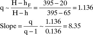
This agrees with Figure 4-10. Despite considerable subcooling this feed line is similar to a saturated liquid feed line. Note that feed rate was not needed to calculate q or the slope for any of these calculations.
4.5 Complete McCabe-Thiele Method
We are now ready to put all the pieces together and solve a design distillation problem by the McCabe-Thiele method. We will do this in the following example.
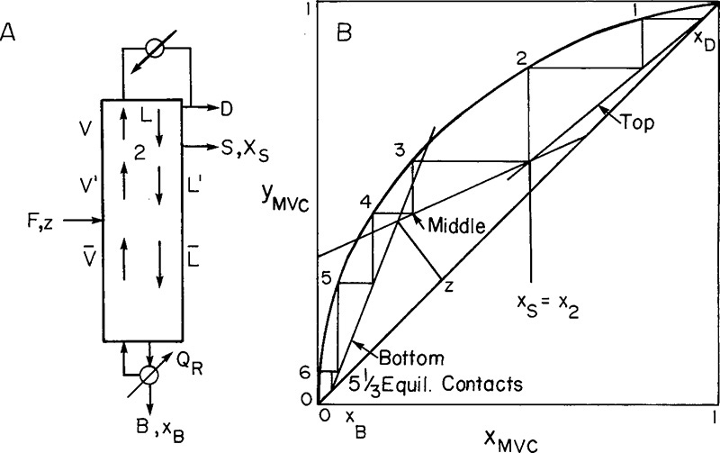
EXAMPLE 4-3. McCabe-Thiele method
A distillation column with a total condenser and a partial reboiler is separating an ethanol-water mixture. Feed is 20.0 mol% ethanol, feed rate is 1000.0 kmol/h, and feed temperature is 80°F. Distillate is 80.0 mol% ethanol, and bottoms is 2.0 mol% ethanol. External reflux ratio is 5/3. Reflux is a saturated liquid, and CMO can be assumed. Pressure is 1.0 atm. Find optimum feed plate location as stages above the reboiler and total number of equilibrium stages.
A. Define. The column is sketched in the following figure.
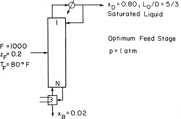
Find the optimum feed plate location and the total number of equilibrium stages.
B. Explore. Equilibrium data at 1 atm are given in Figure 2-2. An enthalpy-composition diagram at 1 atm (Brown et al., 1950, or Foust et al., 1980, p. 36) is helpful to estimate q. However, a good estimate of q can be made from Figure 2-4 despite the pressure difference. In Example 4-1 we showed that CMO is valid. Thus we can apply the McCabe-Thiele method.
C. Plan. Determine q from Eq. (4-17) and the enthalpy-composition diagram at 1 atm. Plot the feed line. Calculate L/V. Plot the top operating line and plot the bottom operating line. Since we want the location of the feed stage above the reboiler, step off stages from the bottom up.
D. Do It. Feed Line: To find q, first convert feed concentration, 20.0 mol%, to wt% ethanol = 39.0 wt%. Two calculations in different units with different data are shown:
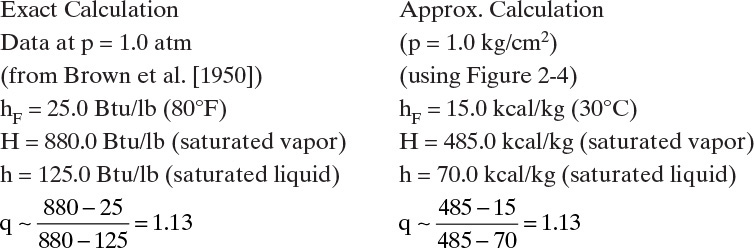
Thus small differences caused by pressure differences in the diagrams do not change the value of q. Note that molecular weight terms divide out as in Example 4-2d. Then
Feed line intersects y = x line at feed concentration z = 0.2 and is plotted in Figure 4-13.
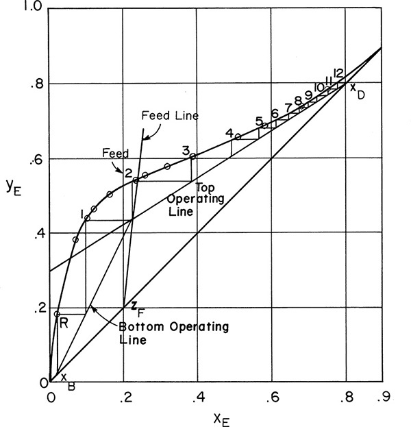
FIGURE 4-13. Solution for Example 4-3
Top Operating Line:
Alternative solution: Intersection of top operating line and y = x (solve top operating line and y = x simultaneously) is at y = x = xD. The top operating line is plotted in Figure 4-13.
Bottom Operating Line:

We know that the bottom operating line intersects the top operating line at the feed line; this intersection is one point. We could calculate ![]() from mass balances or from Eq. (4-25), but it easier to find another point. The intersection of the bottom operating line and the y = x line is at y = x = xB (see Problem 4.C9). This intersection gives a second point.
from mass balances or from Eq. (4-25), but it easier to find another point. The intersection of the bottom operating line and the y = x line is at y = x = xB (see Problem 4.C9). This intersection gives a second point.
The feed line, top operating line, and bottom operating line are shown in Figure 4-13. We stepped off stages from the bottom up. The optimum feed stage is the second above the partial reboiler. Twelve equilibrium stages plus a partial reboiler are required.
E. Check. We have a built-in check on the top operating line since a slope and two points are calculated. The bottom operating line can be checked by calculating ![]() from mass balances and comparing it to the slope. The numbers are reasonable since L/V < 1,
from mass balances and comparing it to the slope. The numbers are reasonable since L/V < 1, ![]() , and q > 1 as expected. We have assumed CMO, which is not completely valid. An appropriate check on this assumption is to compare results with a calculation that does not assume CMO. Usually the most likely cause of significant error in a distillation calculation (and the hardest to check) is the equilibrium data. However, ethanol-water has been studied extensively, and the equilibrium data is accurate.
, and q > 1 as expected. We have assumed CMO, which is not completely valid. An appropriate check on this assumption is to compare results with a calculation that does not assume CMO. Usually the most likely cause of significant error in a distillation calculation (and the hardest to check) is the equilibrium data. However, ethanol-water has been studied extensively, and the equilibrium data is accurate.
F. Generalization. If constructed carefully, the McCabe-Thiele diagram is quite precise. Note that there is no need to plot parts of the diagram that are greater than xD or less than xB. Specified parts of the diagram can be expanded to increase the precision.
We did not use external balances in this example, while we did in Example 4-1,because in this example we used the feed line as an aid in finding the bottom operating line. The y = x intersection points are often useful, but when the column configuration is changed, their location may change.
4.6 Profiles for Binary Distillation
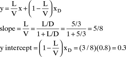
Figure 4-13 essentially shows the complete solution of Example 4-3; however, it is useful to plot compositions, temperatures, and flow rates leaving each stage (these are known as profiles). From Figure 4-13 we can easily find the ethanol mole fractions in the liquid and vapor leaving each stage. Then xW = 1 – xE and yW = 1 – yE. The temperature of each stage can be found from equilibrium data (Figure 2-3) because the stages are equilibrium stages. Since we assumed CMO, the flow rates of liquid and vapor will be constant in the enriching and stripping sections, and we can determine the changes in the flow rates at the feed stage from the calculated value of q.
The profiles are shown in Figure 4-14. As expected, the water concentration in both liquid and vapor streams decreases monotonically as we go up the column, while the ethanol concentration increases. Since ethanol is more volatile, the temperature decreases monotonically as we go up the column. The profiles are not smooth curves because the stages are discrete. When the operating line and equilibrium curve almost touch in Figure 4-13, we have a pinch point. In the profiles pinch points show almost no change in composition and temperature from stage to stage (Figure 4-14). In this ethanol-water column the temperature decreases rapidly for the first few trays above the reboiler but is almost constant for the last eight stages. The location of a pinch point within the column depends on the system and the operating conditions.
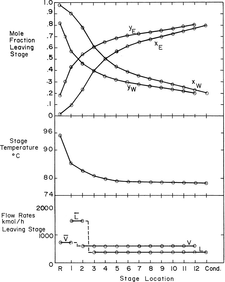
FIGURE 4-14. Profiles for Example 4-3
Since we assumed CMO, the flow profiles are flat in each section of the column. As expected, ![]() and V > L (a convenient check). Since stage 2 is the feed stage, L2 is in the stripping section, and V2 is in the enriching section (draw a sketch of the feed stage if this distinction is not clear). Different quality feeds have different changes at the feed stage. Liquid and vapor flow rates can increase, decrease, or remain unchanged in passing from the stripping to the enriching section.
and V > L (a convenient check). Since stage 2 is the feed stage, L2 is in the stripping section, and V2 is in the enriching section (draw a sketch of the feed stage if this distinction is not clear). Different quality feeds have different changes at the feed stage. Liquid and vapor flow rates can increase, decrease, or remain unchanged in passing from the stripping to the enriching section.
Figure 4-13 illustrates the main advantage of McCabe-Thiele diagrams. They allow us to visualize the separation. Before the common use of digital computers, large (sometimes covering a wall) McCabe-Thiele diagrams were used to design distillation columns. McCabe-Thiele diagrams cannot compete with the speed and accuracy of process simulators (see this chapter’s Appendix A) or, for binary separations, with spreadsheets; however, McCabe-Thiele diagrams still provide superior visualization of the separation (Kister, 1995). Ideally, McCabe-Thiele diagrams are used in conjunction with process simulator results for both analysis and troubleshooting.
4.7 Open Steam Heating
We now have all the tools required to solve any binary distillation problem with the graphical McCabe-Thiele procedure. As a specific example, consider the separation of methanol from water in a staged distillation column.
EXAMPLE 4-4. McCabe-Thiele analysis of open steam heating
A 60.0 mol% methanol and 40.0 mol% water feed is input as a two-phase mixture that flashes so that VF/F = 0.3. Feed flow rate is 350.0 kmol/h. The column is well insulated and has a total condenser. The reflux is returned to the column as a saturated liquid. An external reflux ratio of L0/D = 3.0 is used. We desire a distillate concentration of 95.0 mol% methanol and a bottoms concentration of 8.0 mol% methanol. Instead of using a reboiler, saturated steam at 1.0 atm is sparged directly into the bottom of the column to provide boilup (called direct or open steam). Column pressure is 1 atm. Calculate the number of equilibrium stages and the optimum feed plate location.
A. Define. It is helpful to draw a schematic diagram of the apparatus, particularly since a new type of distillation is involved, as shown in Figure 4-15. We wish to find the optimum feed plate location, NF, and the total number of equilibrium stages, N, required for this separation. We could also calculate Qc, D, B, and the steam rate S, but these are not asked for. We assume that the column is adiabatic since it is well insulated.
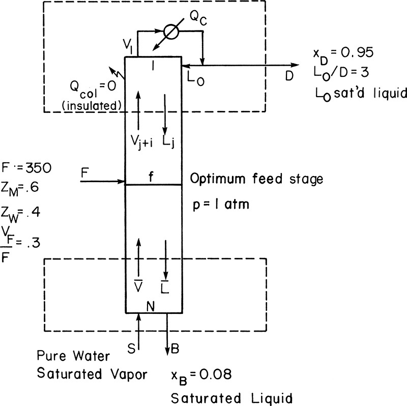
FIGURE 4-15. Distillation with direct steam heating, Example 4-4
B. Explore. The first thing we need is equilibrium data. Fortunately, these are readily available (see Table 2-7 in Problem 2.D1).
Second, we would like to assume CMO so that we can use the McCabe-Thiele analysis procedure. An easy way to check this assumption is to compare the latent heats of vaporization per mole (Himmelblau, 1974):
ΔHvap methanol (at boiling point) = 8.43 kcal/mol
ΔHvap water (at boiling point) = 9.72 kcal/mol
These values are not equal, and in fact water’s latent heat is 15.3% higher than methanol’s. Thus CMO is not strictly valid; however, we will solve this problem assuming CMO and check our results with a process simulator.
A look at Figure 4-15 shows that the configuration at the bottom of the column is different than when a reboiler is present. Thus we should expect that the bottom operating equations will be different from those derived previously.
C. Plan. We will use a McCabe-Thiele analysis. Plot the equilibrium data on a y-x graph.
Top Operating Line: Mass balances in the rectifying section (see Fig. 4-15) are
Vj+1 = Lj + D
yj+1Vj+1 = Lj xj +DxD
Assume CMO and solve for yj+1:
yj+1 = (L/V)xj + (1 – L/V)xD
Slope = L/V, y intercept (x = 0) = (1 – L/V) xD
Intersection y = x= xD
Since the reflux is returned as a saturated liquid,
Enough information is available to plot the top operating line.
Feed Line:
Once we substitute in values, we can plot the feed line.
Bottom Operating Line: The overall and methanol mass balances are
Solve for y:
Simplifications: Since the steam is pure water vapor, yS = 0.0 (contains no methanol). Since steam is saturated, S = V and B = L (constant molal overflow). Then
Note this is different from the operating equation for the bottom section when a reboiler is present. ![]() ,
, ![]() , and
, and
One known point is the intercept of the top operating line with the feed line. We still need a second point, and we can find it at the x intercept. When y is set to zero, x = xB (this is left as Problem 4.C1).
D. Do It. Equilibrium data are plotted on Figure 4-16.
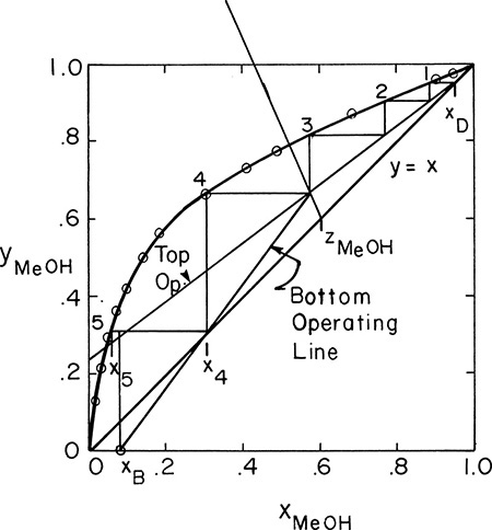
FIGURE 4-16. Solution for Example 4-4
y = x = xD = 0.95
y intercept = (1 – L/V)xD = 0.2375
We can plot this straight line as shown in Figure 4-16.
Feed Line: Slope = q/(q – 1) = 0.7/(0.7 – 1) = –7/3.
Intersects at y = x = z = 0.6.
Bottom Operating Line: We can plot this line between two points, the intercept of top operating line and feed line and
x intercept (y = 0) = xB = 0.08
This is also shown in Figure 4-16.
Step off stages, starting at the top. x1 is in equilibrium with y1 at xD. Drawing a horizontal line to the equilibrium curve gives value x1. y2 and x1 are related by the operating line. At a constant value of y2 (horizontal line), go to the equilibrium curve to find x2. Continue this stage-by-stage procedure.
Optimum feed stage is determined as in Figure 4-8A. Optimum feed in Figure 4-16 is on stage 3 or 4 (since by accident x3 is at intersection point of feed and operating lines). Since the feed is a two-phase feed, we would introduce it above stage 4.
Number of stages: Five is more than enough. We can calculate a fractional number of stages.

In Figure 4-16
We need 4 + 0.9 = 4.9 equilibrium contacts.
E. Check. There are a series of internal consistency checks that can be made. Equilibrium should be a smooth curve. This will pick up incorrectly plotted points. L/V < 1 (otherwise no distillate product) and ![]() (otherwise no bottoms product). The feed line’s slope is in the correct direction for a two-phase feed. A final check on the assumption of CMO is advisable since the latent heats vary by 15%.
(otherwise no bottoms product). The feed line’s slope is in the correct direction for a two-phase feed. A final check on the assumption of CMO is advisable since the latent heats vary by 15%.
This problem was also run on the Aspen Plus process simulator (see Problem 4.G1 and this chapter’s Appendix A). Aspen Plus does not assume CMO and, with an appropriate vapor-liquid equilibrium (VLE) correlation (the nonrandom two-liquid [NRTL] model was used), should be more accurate than the McCabe-Thiele diagram, which assumes CMO. With five equilibrium stages and feed on stage 4 (the optimum location), xD = 0.9335 and xB = 0.08365, which does not meet the specifications. With six equilibrium stages and feed on stage 5 (the optimum), xD = 0.9646 and xB = 0.0768, which is slightly better than the specifications. The differences in the McCabe-Thiele and process simulation results are due to the error involved in assuming CMO and, to a lesser extent, differences in equilibrium. Note that the McCabe-Thiele diagram is useful since it visually shows the effect of using open steam heating.
F. Generalize. Note that the y = x line is not always useful. Do not memorize locations of points; learn to derive what is needed. The total condenser does not change compositions and is not counted as an equilibrium stage. The total condenser appears in Figure 4-16 as the single point y = x = xD. Think about why this is true. In general, all inputs to the column can change flow rates and hence slopes inside the column. The purpose of the feed line is to help determine this effect. The reflux stream and open steam are also inputs to the column. If they are not saturated streams the flow rates are calculated differently; this topic is discussed later.
Note that the open steam can be treated as a feed with ![]() . Thus,
. Thus, ![]() . The slope of this feed line is q/(q – 1) = 0, and it intersects the y = x line at y = x = z = 0, which means the feed line for saturated steam is the x-axis.
. The slope of this feed line is q/(q – 1) = 0, and it intersects the y = x line at y = x = z = 0, which means the feed line for saturated steam is the x-axis.
Ludwig (1997) states that one tray is used to replace the reboiler and one-third to one and possibly more trays to offset the water dilution; however, since reboilers are typically much more expensive than trays (see Chapter 11), this practice is economical. Open steam heating can be used even if water is not one of the original components.
Note to Students: When you read the description of developing the bottom operating equation and plotting the bottom operating line in Example 4-4, it probably appears easier than doing the development by yourself will prove to be. You need to practice deriving operating equations. Then practice simplifying the operating equation, realizing that “pure steam” means yS = 0 and that “saturated steam” means ![]() , and thus
, and thus ![]() are nontrivial steps. How did we know that the bottom operating line could be plotted using the point x = 0 (the y intercept)? We did not know this in advance, but tried it and it worked. You will become better at solving these problems as you work additional problems. To aid in this development, there are numerous problems at the end of this chapter.
are nontrivial steps. How did we know that the bottom operating line could be plotted using the point x = 0 (the y intercept)? We did not know this in advance, but tried it and it worked. You will become better at solving these problems as you work additional problems. To aid in this development, there are numerous problems at the end of this chapter.
4.8 General McCabe-Thiele Analysis Procedure
The open steam example illustrated one specific case. It is useful to generalize this analysis procedure. A section of the column is the segment of stages between two input or exit streams. Thus in Figure 4-15 there are two sections: top and bottom. Figure 4-17 illustrates a column with four sections. Each section’s operating equation can be derived independently. Thus the secret (if that’s what it is) is to treat each section as an independent sub problem connected to the other sub problems by the feed lines (which are also independent).
An algorithm for any problem is the following:
1. Draw a figure of the column, and label all known variables (e.g., as in Figure 4-15). Check to see if CMO is valid.
2. For each section:
a. Draw a mass balance envelope. We desire this envelope to cut the unknown liquid and vapor streams in the section and known streams (feeds, specified products or specified side-streams). The fewer streams involved, the simpler the mass balances will be. This step is important since it controls how easy the following steps will be.
b. Write the overall and MVC mass balances.
c. Derive the operating equation.
d. Simplify.
e. Calculate all known slopes, intercepts, and intersections.
3. Develop feed line equations. Calculate q values, slopes, and y = x intersections.
4. For operating and feed lines:
a. Plot as many of the operating lines and feed lines as you can.
b. If all operating lines cannot be plotted, step off stages if the stage location of any feed or side stream is specified.
c. If needed, do external mass and energy balances (see Example 4-5). Use the values of D and B in step 2.
5. When all operating lines have been plotted, step off stages and determine the optimum feed plate locations and the total number of stages. If desired, calculate a fractional number of stages.
Not all of these general steps are illustrated in the previous examples, but they are illustrated in the examples that follow.
This problem-solving algorithm should be used as a guide, not as a computer code to be followed exactly. The wide variety of possible configurations for distillation columns allows for plenty of problem-solving practice using the McCabe-Thiele method.
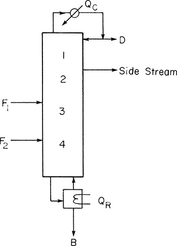
EXAMPLE 4-5. Distillation with two feeds
We wish to separate ethanol from water in a distillation column with a total condenser and a partial reboiler. We have 200.0 kmol/h of feed 1, which is 30.0 mol% ethanol and is saturated vapor. We also have 300.0 kmol/h of feed 2, which is 40.0 mol% ethanol. Feed 2 is a subcooled liquid. One mole of vapor must condense inside the column to heat up 4 moles of feed 2 to its boiling point. We desire a bottoms product that is 2.0 mol% ethanol and a distillate product that is 72.0 mol% ethanol. External reflux ratio is L0/D = 1.0. The reflux is a saturated liquid. Column pressure is 101.3 kPa, and the column is well insulated. The feeds are to be input at their optimum feed locations. Find the optimum feed locations (reported as stages above the reboiler) and the total number of equilibrium stages required.
Solution
A. Define. Again a sketch will be helpful (see Figure 4-18). Since the two feed streams are already partially separated, it makes sense to input them separately to maintain the separation that already exists. We have made an inherent assumption in Figure 4-18. That is, feed 2 of higher mole fraction ethanol enters the column higher up than feed 1. This assumption will be checked when the optimum feed plate locations are calculated, but it will affect the way we do the preliminary calculations. Since the feed plate locations were asked for as stages above the reboiler, the stages have been numbered from the bottom up.
FIGURE 4-18. Two-feed distillation column for Example 4-5
B. Explore. Obviously equilibrium data are required, and they are available from Figure 2-2. We already checked (Example 4-1) that CMO is a reasonable assumption. A look at Figure 4-18 shows that the top section is the same as top sections used previously. The bottom section is also familiar. Thus the new part of this problem is the middle section. There will be two feed lines and three operating lines.
C. Plan. We will look at the two feed lines, top operating line, bottom operating line, and middle operating line. The simple numerical calculations will also be done here.
Feed 1: Saturated vapor, q1 = 0, slope = 0, y intercept = z1/(q1 – 1) = 0.3, intersection at y = x = z1 = 0.3.
Feed 2:
The feed stage for feed 2 looks schematically as shown in the figure.
Then, Lbelow feed = L′ = L + F2 + c.
Amount condensed = c = (1/4) F2,
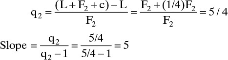
Intersection: y = x = z2 = 0.4
Top Operating Line: We start by deriving the top operating equation
This is the usual top operating line. With saturated liquid reflux the slope is
Intersection: y = x = xD = 0.72
Bottom Operating Line: Next, we derive the bottom operating equation
This is the usual bottom operating line, but slope = ![]() is unknown.
is unknown.
The intersection of the y = x line and the bottom operating line is at y = x = xB = 0.02. One other point is the intersection of the F1 feed line and the middle operating line, if we can find the middle operating line.
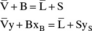
Middle Operating Line: To derive an operating equation for the middle section, we can write a mass balance around the top or the bottom of the column. The resulting equations will look different, but they are equivalent. We arbitrarily use the mass balance envelope around the top of the column, as shown in Figure 4-18. The overall and MVC mass balances are
F2 + V′ = L′ + D
F2z2 + V′ y = L′ x + DxD
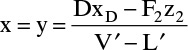
Solve the second equation for y to develop the middle operating equation:
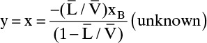
One known point is the intersection of the middle operating line, the F2 feed line and the top operating line. A second point is needed. We can try
However, this point is unknown.
The intersection of the middle operating line with the y = x line is found by setting y = x in Eq. (4-44) and solving
From the overall balance equation,
V′ – L′ = D – F2
Thus
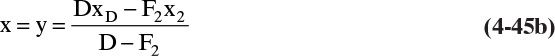
This point is not known, but it can be calculated once D is known.
Slope = L′/V′ is unknown, but it can be calculated from balances at the feed-stage. From the definition of q2,
where L = (L/D)D. Once D is determined, L and then L′ can be calculated. Then the mass balance gives
V′ = L′ + D – F2
and the slope L′/V′ can be calculated.
The conclusion from these calculations is that we have to calculate D. To do this we need external mass balances:
We can solve these two equations for the two unknowns, D and B. Substituting B = F1 + F2 – D into Eq. (4-47b) and solving for D:

This equation is essentially the solution for question 3.C3.
D. Do It. The two feed lines and the top operating line can immediately be plotted on a y-x diagram. This is shown in Figure 4-19. Before plotting the middle operating line we must find D from Eq. (4-48).

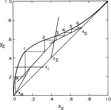
FIGURE 4-19. Solution for Example 4-5
Now the middle operating line y = x intercept can be determined from Eq. (4-45b):
This intersection point could be used, but it is off the graph in Figure 4-19. Instead of using a larger sheet of paper, we will calculate the slope L′/V′.
The middle operating line is plotted in Figure 4-19 from the intersection of feed line 2 and the top operating line, with a slope of 1.10. The bottom operating line then goes from y = x = xB to the intersection of the middle operating line and feed line 1 (see Figure 4-19).
Since the feed locations were desired as stages above the reboiler, we step off stages from the bottom up, starting with the partial reboiler as the first equilibrium contact. The optimum feed stage for feed 1 is the first stage, while the optimum feed stage for feed 2 is the second stage. Six stages + partial reboiler are more than sufficient. If desired, a fractional number of stages can be estimated:
We need 5½ stages and a partial reboiler.
E. Check. The internal consistency checks all make sense. Note that L′/V′ can be greater than or less than 1.0. Since the latent heats of vaporization per mole are close, CMO is probably a good assumption. Our initial assumption that feed 2 enters the column higher up than feed 1 is shown to be valid by the McCabe-Thiele diagram. We could also calculate ![]() and
and ![]() and check that the slope of the bottom operating line is correct.
and check that the slope of the bottom operating line is correct.
F. Generalize. The method of inserting the overall mass balance to simplify the intersection of the y = x line and middle operating line to derive Eq. (4-45) can be used in other cases. The method for calculating L′/V′ can also be generalized to other situations. That is, we can calculate D (or B), find flow rate in the section above (or below), and use feed conditions to find flow rates in the desired section. Since we stepped off stages from the bottom up, the fractional stage is calculated from the difference in y values (i.e., vertical distances) in Eq. (4-49). Although we obviously cannot build fractions of a stage, the calculation can be useful if the column efficiency is low (see Section 4.11). For example, if the overall efficiency is 20%, then 6 equilibrium contacts is 30 real stages, and 5½ equilibrium contacts is 28 real stages. Industrial systems typically use lower reflux ratios and have more stages. A relatively large reflux ratio is used in this example to keep the graph simple.
4.9 Other Distillation Column Situations
A variety of modifications of the basic columns are often used. In this section we briefly consider the unique aspects of several of these variations. CMO is assumed. Detailed examples are not given but are left to serve as homework problems.
4.9.1 Partial Condensers
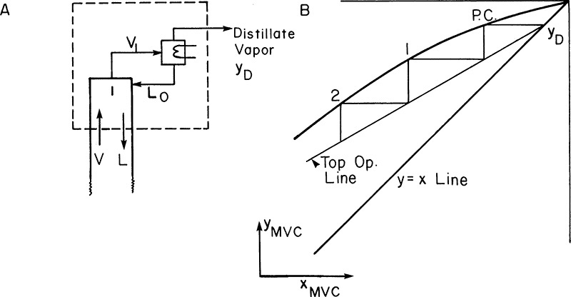
A partial condenser condenses only part of the overhead stream and returns this as reflux. This distillate product is removed as vapor, as shown in Figure 4-20. If a vapor distillate is desired, then a partial condenser is convenient. The partial condenser acts as one equilibrium contact.
If a mass balance is done on the MVC using the mass balance envelope shown in Figure 4-20, we obtain
Vy = Lx + DyD
Substituting in D = V – L and solving for y, we obtain the operating equation
This is essentially the same as the equation for a top operating line with a total condenser except that yD has replaced xD. The top operating line will intersect the y = x line at y = x = yD. The top operating line is shown in Figure 4-20. The major difference between this case and that in the figure for a total condenser is that the partial condenser serves as the first equilibrium contact.
4.9.2 Total Reboilers
A total reboiler vaporizes the entire stream sent to it; thus the vapor composition is the same as the liquid composition. This scenario is illustrated in Figure 4-21. The mass balance and the bottom operating equation with a total reboiler are exactly the same as with a partial reboiler (Problem 4.C2). The only difference is that a partial reboiler is an equilibrium contact and is labeled as such on the McCabe-Thiele diagram. The total reboiler is not an equilibrium contact and appears on the McCabe-Thiele diagram as the single point y = x = xB.
Some types of partial reboilers may act as more or less than one equilibrium contact. In these cases, exact details of the reboiler construction are required.
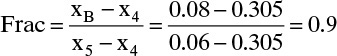
4.9.3 Side Streams or Withdrawal Lines
If a product of intermediate composition is required, a vapor or liquid side stream may be withdrawn. This is commonly done in petroleum refineries and is illustrated in Figure 4-22A for a liquid side stream. Three additional variables, such as type of side draw (liquid or vapor), flow rate, SL or SV, and location or composition xS or yS, must be specified. The operating equation for the middle section can be derived from mass balances around the top or bottom of the column. For the situation shown in Figure 4-22A, the middle operating equation is
The y = x intercept is

This point can be plotted if SL, xS, D, and xD are known. Derivation of Eqs. (4-51) and (4-52) is left as Problem 4.C3.
A second point can be found where the side stream is withdrawn. A saturated liquid withdrawal is equivalent to a negative feed of concentration xS. Thus there must be a vertical feed line at x = xS. The top and middle operating lines must intersect at this feed line.
Side-stream calculations have one difference that sets them apart from feed calculations. The stage must hit exactly at the point of intersection of the two operating lines. This is illustrated in Figure 4-22B. Since the liquid side stream is withdrawn from tray 2, we must have xS = x2. If stage location is given, xS can be found by stepping off the required number of stages.
For a liquid withdrawal, vapor flow rates are unchanged, V = V′, and a balance on the liquid gives
Thus slope, L′/V′, of the middle operating line can be determined if L and V are known. L and V can be determined from L/D and D, where D can be found from external balances once xS is known.
For a vapor side stream, the feed line is horizontal at y = yS, which is equivalent to a negative horizontal feed line for a saturated vapor. A balance on vapor flow rates gives
and liquid flow rates are unchanged. Again L′/V′ can be calculated if L and V are known.
If a specified value of xS (or yS) is desired, the problem is trial and error. The top operating line is adjusted (change L/D) until a stage ends exactly at xS or yS.
Calculations for side streams below the feed can be developed using similar principles (Problem 4.C4).
4.9.4 Intermediate Reboilers and Intermediate Condensers
Another modification that is used occasionally is to have an intermediate reboiler or an intermediate condenser. The intermediate reboiler removes a liquid side stream from the column, vaporizes it, and reinjects the vapor into the column. An intermediate condenser removes a vapor side stream, condenses it, and reinjects it into the column. Figure 4-23A illustrates an intermediate reboiler.
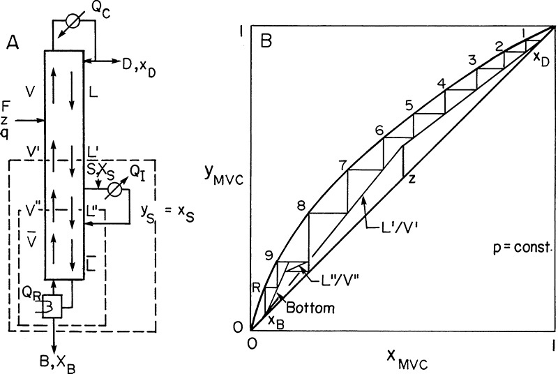
An energy balance around the column will show that QR without an intermediate reboiler is equal to QR + QI with the intermediate reboiler (F, z, q, xD, xB, p, L/D constant). Thus the amount of energy required is unchanged; what changes is the temperature at which it is required. Since xS > xB, the temperature of the intermediate reboiler is lower than that of the reboiler, and a lower temperature and hence cheaper heat source often can be used. (Check this out with equilibrium data.)
Since the column shown in Figure 4-23A has four sections, there will be four operating lines. This is illustrated in the McCabe-Thiele diagram of Figure 4-23B. We would specify that the liquid be withdrawn at flow rate S at either a specified concentration xS or a given stage location. The saturated vapor is at concentration yS = xS. Thus there is a horizontal feed line at yS. If the optimum location for inputting the vapor is immediately below the stage where the liquid is withdrawn, the L″/V″ line will be present, but no stages will be stepped off on it, as shown in Figure 4-23B. (The optimum location for vapor feed may be several stages below the liquid withdrawal point.) Development of the two middle operating lines is left as Problem 4.C5. Use the mass balance envelopes shown in Figure 4-23A to solve that problem.
Intermediate condensers are useful since the coolant can be at a higher temperature (see Problem 4.C6). Intermediate reboilers and condensers are fairly common because they allow for more optimum use of energy resources, and they can help balance column diameters (see Section 10.4). During normal operation they should cause no problems; however, startup may be difficult (Sloley, 1996).
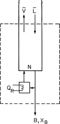
4.9.5 Stripping and Enriching Columns
Up to this point we have considered complete distillation columns with at least two sections. Columns with only a stripping section or only an enriching section are also commonly used. These are illustrated in Figures 4-24A and 4-24B. When only a stripping section is used, the feed must be a subcooled or saturated liquid. No reflux is used. A very pure bottoms product can be obtained, but the vapor distillate will not be pure. In the enriching or rectifying column, on the other hand, the feed is a superheated vapor or a saturated vapor, and the distillate can be very pure, but the bottoms will not be very pure. Striping columns and enriching columns are used when a pure distillate or a pure bottoms, respectively, is not needed.
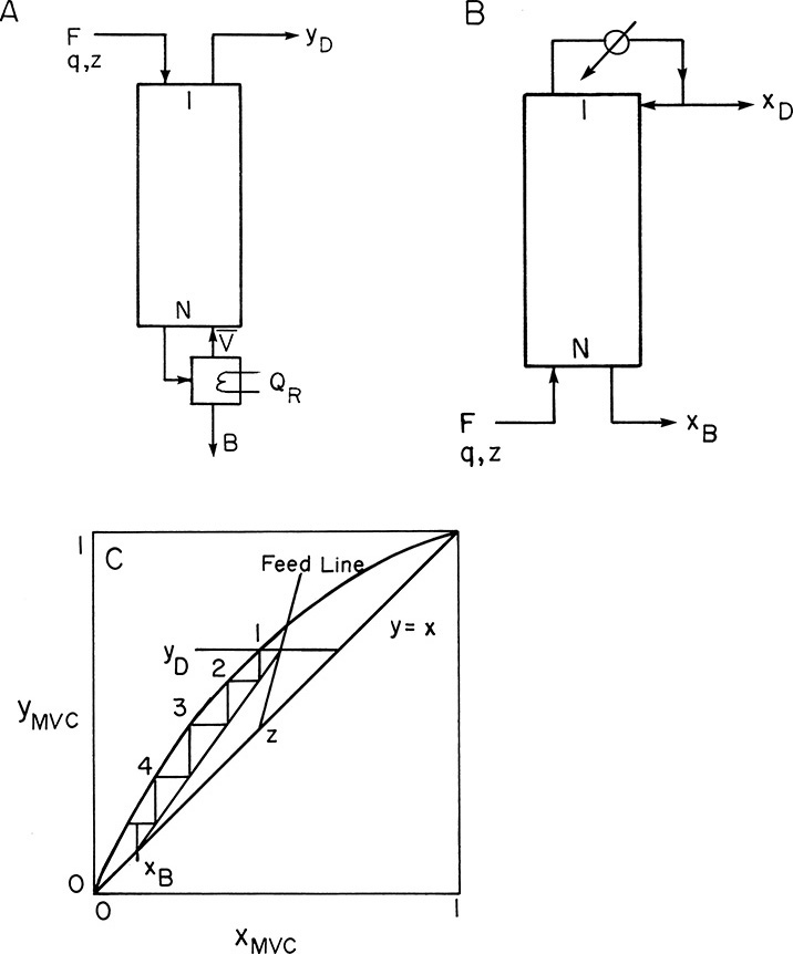
FIGURE 4-24. Stripping and enriching columns; (A) stripping, (B) enriching, (C) McCabe-Thiele diagram for stripping column with subcooled feed
Analysis of stripping and enriching columns is similar. We will analyze the stripping column here and leave the analysis of the enriching column as a homework assignment (Problem 4.C8). The stripping column shown in Figure 4-24A can be thought of as a complete distillation column with zero liquid flow rate in the enriching section. Then the top operating line is y = yD. The bottom operating line can be derived as
which is the usual equation for a bottom operating equation with a partial reboiler. Top and bottom operating lines intersect at the feed line. If the specified variables are F, q, z, p, xB, and yD, the feed line can be plotted and then the bottom operating line can be obtained from its intersection at y = x = xB and its intersection with the feed line at yD. (Proof is left as Problem 4.C7.) If the boilup rate, ![]() , is specified, then yD will not be specified and can be solved for. The McCabe-Thiele diagram for a stripping column is shown in Figure 4-24C.
, is specified, then yD will not be specified and can be solved for. The McCabe-Thiele diagram for a stripping column is shown in Figure 4-24C.
Stripping and enriching columns have one less degree of freedom than complete columns. This is easy to see when CMO is valid. In stripping columns the liquid flow rate ![]() and the vapor flow rate
and the vapor flow rate ![]() . Thus, the boilup rate
. Thus, the boilup rate ![]() cannot be adjusted independently. In enriching columns the reflux ratio L/D = F/D cannot be adjusted independently.
cannot be adjusted independently. In enriching columns the reflux ratio L/D = F/D cannot be adjusted independently.
4.10 Limiting Operating Conditions
It is always useful to look at limiting conditions. For distillation, two limiting conditions are total reflux and minimum reflux. In total reflux (Figure 4-25A) all overhead vapor is returned to the column as reflux, and all underflow liquid is returned as boilup; thus, distillate and bottoms flow rates are zero. At steady state the feed rate must also be zero. Total reflux is used for starting up columns, for keeping a column operating when another part of the plant is shut down, and for testing column efficiency.
The analysis of total reflux is simple. Since all vapor is condensed and refluxed, L = V and L/V = 1.0. Also, ![]() and
and ![]() Thus both operating lines become the y = x line (Figure 4-25B). Total reflux represents the maximum separation that can be obtained with a given number of stages but zero throughput. Total reflux also gives the minimum number of stages required for a given separation. Although simple, total reflux can cause safety problems. Leakage near the top of the column can cause concentration of high boilers with a corresponding increase in temperature. This can result in polymerization, fires, or explosions (Kister, 1990). Thus the temperature at the top of the column should be monitored, and an alarm should sound if this temperature becomes too high.
Thus both operating lines become the y = x line (Figure 4-25B). Total reflux represents the maximum separation that can be obtained with a given number of stages but zero throughput. Total reflux also gives the minimum number of stages required for a given separation. Although simple, total reflux can cause safety problems. Leakage near the top of the column can cause concentration of high boilers with a corresponding increase in temperature. This can result in polymerization, fires, or explosions (Kister, 1990). Thus the temperature at the top of the column should be monitored, and an alarm should sound if this temperature becomes too high.
Minimum reflux, (L/D)min, is defined as the external reflux ratio at which the desired separation could just be obtained with an infinite number of stages. This is obviously not a real condition, but it is a useful hypothetical construct. To have an infinite number of stages, the operating and equilibrium lines must touch. In general, this can happen either at the feed or at a point tangent to the equilibrium curve. These two points are illustrated in Figures 4-26A and 4-26B. The point where the operating line touches the equilibrium curve is called the pinch point. At the pinch point the concentrations of liquid and vapor do not change from stage to stage. This pinch at the feed stage is illustrated in Figure 4-26C. If the reflux ratio is increased slightly, then the desired separation can be achieved with a finite number of stages.
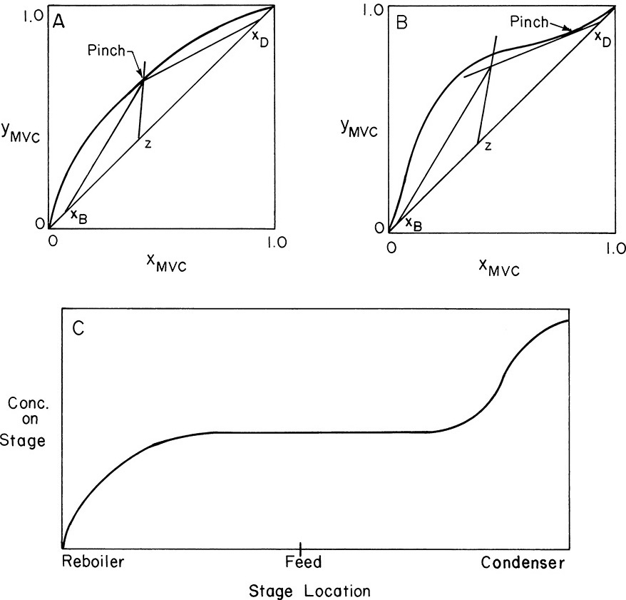
FIGURE 4-26. Minimum reflux; (A) pinch at feed stage, (B) tangent pinch, (C) concentration profile for L/D ∼ (L/D)min
For binary systems the minimum reflux ratio is easily determined. The top operating line is drawn to a pinch point, as in Figures 4-26A and 4-26B. Then (L/V)min is equal to the slope of this top operating line (which cannot be used for an actual column, since an infinite number of stages are needed):
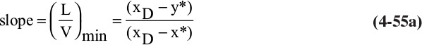
where (y*, x*) are the coordinates of the intersection of the feed line and the equilibrium curve. Once (L/V)min is known,

Note that the minimum reflux ratio depends on xD, z, and q and can depend on xB. The calculation of minimum reflux may be more complex when there are two feeds or a sidestream. This is explored in the homework problems.
The minimum reflux ratio is commonly used in specifying operating conditions. For example, we may specify the reflux ratio as L/D = 1.2(L/D)min. Minimum reflux uses the minimum amount of reflux liquid and hence the minimum amount of heat in the reboiler, but it uses the maximum (infinite) number of stages and a maximum (infinite) diameter for a given separation. Obviously the best operating conditions lies somewhere between minimum and total reflux. As a rule of thumb the optimum external reflux ratio for a column with enriching and stripping sections is between 1.05 and 1.25 times (L/D)min. (See Chapter 11 for more details.)
A maximum ![]() and hence a minimum boilup ratio
and hence a minimum boilup ratio ![]() can also be defined. The pinch points will look the same as in Figures 4-26A and 4-26B. Problem 4.C12 looks at this situation further.
can also be defined. The pinch points will look the same as in Figures 4-26A and 4-26B. Problem 4.C12 looks at this situation further.
When the feed is a saturated liquid, x* = z and y* can be calculated from the relative volatility Eq. (2-22b) with x = z. The resulting equation for L/D can be simplified in the limit of perfect separation (xD → 1 and xB → 0) to

where α is the relative volatility calculated at x = z. For a saturated vapor feed the limiting case result is

where the relative volatility α is calculated at y = z. These equations indicate that very high purity requirements do not cause a large increase in the reflux ratio. Instead, significantly more stages are required (King, 1980).
4.11 Efficiencies
Until now we have always assumed that the stages are equilibrium stages. Stages that are very close to equilibrium can be constructed, but they are used only for special purposes, such as determining equilibrium concentrations. To compare the performance of an actual stage to an equilibrium stage, we use a measure of efficiency.
Many different measures of efficiency have been defined. Two that are in common use are the overall efficiency and the Murphree efficiency. The overall efficiency, Eo, is defined as the number of equilibrium stages required for the separation divided by the actual number of stages required:
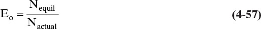
Partial condensers and partial reboilers are not included in either the actual or the equilibrium number of stages since they will not have the same efficiency as the stages in the column.
The overall efficiency lumps together everything that happens in the columns. What variables would we expect to affect column efficiency? The hydrodynamic flow properties, such as viscosity and gas flow rate, affect the flow regime, which affects efficiency. The mass transfer rate, which is affected by the diffusivity, in turn affects efficiency. Overall efficiency is usually smaller as the separation becomes easier (αAB increases). The column size can also have an effect. Correlations for determining the overall efficiency are discussed in Chapter 10. For now we consider how the overall efficiency is determined from operating experience with similar distillation columns.
The overall efficiency has the advantage of being easy to measure and to use, but it has the disadvantage that it is difficult to calculate from first principles. Stage efficiencies are defined for each stage and may vary from stage to stage. The stage efficiencies are easier to estimate from first principles or to correlate with operating data. The most commonly used stage efficiencies for binary distillation are the Murphree vapor and liquid efficiencies (Murphree, 1925). The Murphree vapor efficiency is defined as

Murphree postulated that the vapor between trays is well mixed, that the liquid in the downcomers is well mixed, and that the liquid on the tray is well mixed and is of the same composition as the liquid in the downcomer leaving the tray. For the nomenclature illustrated in Figure 4-27A, the Murphree vapor efficiency is
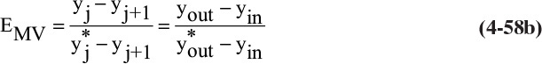
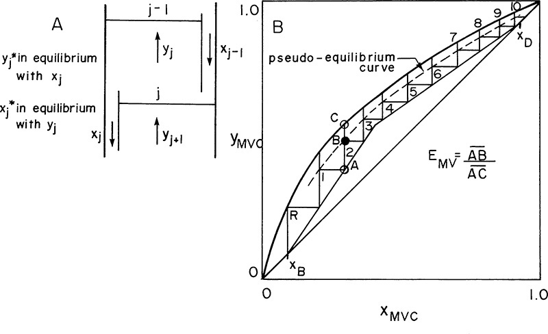
where ![]() is vapor mole fraction in equilibrium with actual liquid mole fraction xj.
is vapor mole fraction in equilibrium with actual liquid mole fraction xj.
Once the Murphree vapor efficiency is known for every stage, it can easily be used on a McCabe-Thiele diagram. (In fact, Murphree adjusted his paper to use the newly developed McCabe-Thiele diagram.) The denominator in Eq. (4-58b) represents vertical distance from operating line to equilibrium line. The numerator is vertical distance from operating line to actual outlet concentration. Thus Murphree vapor efficiency is the fractional amount of total vertical distance from operating line to equilibrium curve to move from yin on operating line to yout. Stepping off stages from the bottom up produces the result shown in Figure 4-27B. Note that the partial reboiler is treated separately since it will have a different efficiency than trays.
Murphree efficiency can be used as a ratio of distances, as shown in Figure 4-27B. If Murphree efficiencies are accurate, locations labeled by stage numbers represent actual vapor and liquid compositions leaving a stage. These points can be connected to form a pseudo-equilibrium curve, but this curve depends on operating lines used and thus has to be redrawn for each new set of operating lines. Figure 4-27B allows us to calculate a real optimum feed plate location and real total number of stages.
A Murphree liquid efficiency can be defined as

which is actual change in liquid mole fraction divided by change for an equilibrium stage. Murphree liquid efficiency is similar to Murphree vapor efficiency except that it uses horizontal distances. Note that EML ≠ EMV.
For binary mixtures Murphree efficiencies are identical whether they are written in terms of MVC or LVC. For multicomponent mixtures Murphree efficiencis are not as useful since they are different for different components and can be negative.
4.12 Simulation Problems
In a simulation problem the column has already been built, and we want to know how much separation can be obtained. As noted in Tables 3-1 and 3-3, the real number of stages, the real feed location, the column diameter, and the types and sizes of reboiler and condenser are known. The engineer does the detailed stage-by-stage calculation and the detailed diameter calculation, and finally he or she checks that the operation is feasible.
To be specific, consider the column in Figure 4-28A in which the known variables are F, z, q, xD, Treflux (saturated liquid), p, Qcol = 0, Nactual, Nfeed actual, diameter, L0/D, the overall efficiency Eo, and CMO. The engineer wishes to determine the bottoms composition, xB.
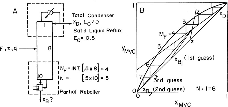
We start by deriving the top and bottom operating equations. These are the familiar forms:
and
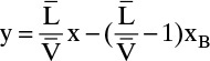
The feed line equation is also unchanged:
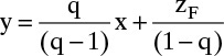
Since the reflux is a saturated liquid and the external reflux ratio, L0/D, is known, we calculate L/V and plot the top operating line (Figure 4-28B). The feed line can also be plotted. The intersection of the top operating line and the feed line gives one point on the bottom operating line. Unfortunately, the bottom operating line cannot be plotted because neither ![]() nor xB is known (why do external balances not give one of these variables?).
nor xB is known (why do external balances not give one of these variables?).
To proceed we must use the three items of information that have not yet been used. These are Nactual, Nfeed actual, and Eo. We can estimate the equilibrium number of stages as
The feed location in equilibrium stages, NF, must be estimated as an integer, but the total number of equilibrium stages, N, could include a fraction. Now we can step off equilibrium stages on the top operating line until we reach the feed stage NF. At this point we need to switch to the bottom operating line, which is not known. To use the final bit of information, the value N, we must guess xB or ![]() , plot the bottom operating line, and check to see if the separation is achieved with N + 1 (the +1 includes the partial reboiler) equilibrium contacts. Thus the simulation problem is one of trial and error when a stage-by-stage computation procedure is used. This procedure is illustrated in Figure 4-28B. The actual feed stage probably is not at the optimum location.
, plot the bottom operating line, and check to see if the separation is achieved with N + 1 (the +1 includes the partial reboiler) equilibrium contacts. Thus the simulation problem is one of trial and error when a stage-by-stage computation procedure is used. This procedure is illustrated in Figure 4-28B. The actual feed stage probably is not at the optimum location.
Once xB or ![]() has been determined, the external balances can be completed, and we can determine B, D, Qc, and QR. L, V,
has been determined, the external balances can be completed, and we can determine B, D, Qc, and QR. L, V, ![]() , and
, and ![]() can be calculated, and we can proceed to check that V and
can be calculated, and we can proceed to check that V and ![]() are less than Vmax. This check is done by a procedure similar to calculating the diameter for a flash drum and is shown in Chapter 10. The condenser and reboiler sizes can also be checked. If the flow rates are too large or the condenser and reboiler are too small, the existing system will not satisfactorily perform the desired separation. Either the feed rate can be decreased or L/D can be decreased. This latter change obviously requires that the entire solution be repeated.
are less than Vmax. This check is done by a procedure similar to calculating the diameter for a flash drum and is shown in Chapter 10. The condenser and reboiler sizes can also be checked. If the flow rates are too large or the condenser and reboiler are too small, the existing system will not satisfactorily perform the desired separation. Either the feed rate can be decreased or L/D can be decreased. This latter change obviously requires that the entire solution be repeated.
When other variables are specified, the stage-by-stage calculation is still trial and error. The basic procedure remains the same. That is, calculate and plot everything you can first, guess the needed variable, and then check whether the separation can be obtained with the existing number of stages. Murphree stage efficiencies are easily employed in these calculations.
Simulation problems are easier to do using a simulator developed for simulation problems (see Appendix A).
4.13 New Uses for Old Columns
Closely related to simulation is the use of existing or used distillation systems for new separations. The new use may be debottlenecking—that is, increasing capacity for the same separation. With increasing turnover of products, the problem of using equipment for new separations is becoming more common.
Why would we want to use an existing column for a problem it was not designed for? First, it is usually cheaper to modify a column that has already been paid for than to buy a new one. Second, it is usually quicker to perform minor modifications than to wait for construction of a new column. Finally, for many engineers solving the often knotty problems involved in adapting a column to a new separation is an interesting challenge.
The first thing to do when new chemicals are to be separated is clean the entire system and inspect it thoroughly. Is the system in good shape? If not, will minor maintenance and parts replacement put the equipment in working order? If there are major structural problems, such as major corrosion, it will probably be cheaper, safer, and less of a long-term headache to buy new equipment.
Do simulation calculations to determine how close the column will come to meeting the new separation specifications. Rarely does the column provide a perfect answer to the new problem. Difficulties can be classified as problems with the separation required and problems with capacity.
What can be done if the existing column cannot produce the desired product purities? The following steps can be explored (they are listed roughly in the order of increasing cost):
1. Find out whether the product specifications can be relaxed. A purity of 99.5% is much easier to obtain than 99.99%.
2. See if a higher reflux ratio will do the separation. Remember to check if column vapor capacity and the reboiler and condenser are large enough. If they are, then changes in L/D affect only operating costs.
3. Change the feed temperature. This may make a nonoptimum feed stage optimum.
4. Will a new feed stage at the optimum location (the existing feed stage is probably nonoptimum) allow you to meet product specifications?
5. Consider replacing the existing trays (or packing) with more efficient or more closely spaced trays (or new packing). This solution is relatively expensive but is cheaper than buying a completely new system.
6. Check to see if two existing columns can be hooked together in series to achieve the desired separation. Feed can be introduced at the feed tray of either column or in between the two columns. Since vapor loading requirements are different in different sections of the column (see Chapter 10), the columns do not have to be the same diameter.
What if the column produces product much purer than specifications? This situation is pleasant because the reflux ratio usually can be decreased, which decreases operating expenses.
Problems with vapor capacity are discussed in more detail in Chapter 10. Briefly, if the column diameter is not large enough, the engineer can consider the following solutions:
1. Operating at a reduced L/D, which reduces vapor velocity. This approach may make it difficult to meet the product specifications.
2. Operating at a higher pressure, which increases the vapor density. Note that the column must be designed for these higher pressures, and the chemicals being separated must be thermally stable.
3. Using two columns in parallel.
4. Replacing the downcomers with larger downcomers (see Chapter 10).
5. Replacing the trays or packing with higher capacity trays or packing. Major increases in capacity are unlikely.
If the column diameter is too large, vapor velocities will be low. The trays will operate at tray efficiencies lower than designed, and in severe cases they may not operate at all since liquid may dump through the holes. Possible solutions include
1. Decreasing column pressure to decrease vapor density, which increases the linear vapor velocity.
2. Covering some of the holes if the column has sieve trays, which increases the vapor velocity in the open holes and reduces weeping.
3. Increasing L/D to increase V.
4. Recycling some distillate and bottoms product to effectively increase F.
Using existing columns for new uses often requires a creative solution. Such problems can be both challenging and fun; they are also often assigned to engineers just out of school.
4.14 Subcooled Reflux and Superheated Boilup
What happens if the reflux liquid is subcooled or the boilup vapor is superheated? We have already looked at two similar cases in which we have a subcooled liquid or a superheated vapor feed. In those cases we found that a subcooled liquid condenses some vapor in the column, while a superheated vapor vaporizes some liquid. Since reflux and boilup are inputs to the column, we should expect exactly the same behavior if these streams are subcooled or superheated.
Subcooled reflux often occurs if the condenser is at ground level. Then a pump is required to return the reflux to the top of the column. A saturated liquid causes cavitation and over time destroys the pump; thus the liquid must be subcooled if it is to be pumped. To analyze the effect of subcooled reflux, consider the top of the column shown in Figure 4-29. The cold liquid stream, L0, must be heated up to its boiling point. This energy must come from condensing vapor on the top stage, stream c in Figure 4-29. Thus the flow rates on the first stage are different from those in the rest of the rectifying section. CMO is valid in the remainder of the column. The internal reflux ratio in the rectifying column is L1/V2 = L/V, and the top operating line is
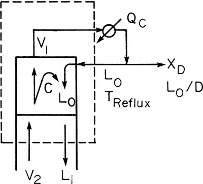
However, L/V cannot be calculated from Eq. (4-26), since L and V change on the top stage.
Balances on vapor and liquid streams give
An energy balance using the balance envelope in Figure 4-29 is
With CMO, H1 ∼ H2. Then Eq. (4-62) becomes
(V2 – V1)H ∼ L1h1 – L0hreflux
Substituting in Eqs. (4-61a, b), this becomes
cH ∼ (L0 + c)h1 – L0hreflux
Solving for amount condensed, c, we obtain

which can also be written as

where fc is the fraction condensed per mole of reflux. We can now calculate the internal reflux ratio, L/V = L1/V2. We start with the ratio we desire and use Eqs. (4-61a and 4-61b) and (4-63):

The ratio L0/V1 is easily found from L0/D as
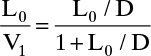
Using this expression in Eq. (4-64) we obtain

Note that when fc = 0, Eqs. (4-64) and (4-65) both simplify to L1/V2 = L0/V1. As the fraction condensed increases (reflux is subcooled more), the internal reflux ratio, L1/V2, becomes larger. Thus the net result of subcooled reflux is equivalent to increasing the reflux ratio. Numerical calculations (such as Problem 4.D5) show that a large amount of subcooling is required to have a significant effect on L/V. If reflux is highly subcooled add an extra tray for heating the reflux (Kister, 1990).
Superheated direct steam input or superheated boilup from a total reboiler causes vaporization of liquid inside the column. This is equivalent to a net increase in the boilup ratio, ![]() , and makes the slope of the stripping section operating line approach 1.0. Since superheated vapor inputs can be analyzed in the same fashion as subcooled liquid reflux, the analysis is left as homework problems 4.C13 and 4.C14.
, and makes the slope of the stripping section operating line approach 1.0. Since superheated vapor inputs can be analyzed in the same fashion as subcooled liquid reflux, the analysis is left as homework problems 4.C13 and 4.C14.
4.15 Comparisons Between Analytical and Graphical Methods
Both the Lewis and McCabe-Thiele methods are based on the CMO assumption. When CMO is valid the energy balances are automatically satisfied, which greatly simplifies stage-by-stage calculations. The reboiler and condenser duties, QR and Qc, are determined from the balances around the entire column. If CMO is not valid, QR and Qc will be unaffected if the same external reflux ratio can be used, but this may not be possible. The exact calculation, which can easily be done with a process simulator, may show that a higher or lower L0/D is required if CMO is invalid.
When a programmable calculator or a computer is to be used, the Lewis analytical method is more convenient, particularly if a spreadsheet is used (Burns and Sung, 1996). Computer calculations are obviously more convenient if a very large number of stages are required, if a trial-and-error solution is required, or if many cases are to be run (e.g., for economic analysis). However, since accuracy is limited by the equilibrium data and the CMO assumption, computer calculations assuming CMO are not more accurate than the graphical method.
If calculations are to be done by hand, the graphical method is faster than alternating between the analytical forms of the equilibrium relationship and the operating equations. In the McCabe-Thiele method, solving the equilibrium relationship is simply a matter of drawing a line to the equilibrium curve. In the analytical solution we must first either fit the equilibrium data to an analytical expression or develop an interpolation routine. Then we must solve this equation, which may be nonlinear, each time we do an equilibrium calculation. Since the operating equation is linear, it is easy to solve analytically. With a sharp pencil, large graph paper, and care, the McCabe-Thiele technique can be as accurate as the equilibrium data (typically two significant figures).
When doing analytical stage-by-stage calculations from the top down, we solve for x values from the equilibrium relationship and for y values from the operating equation. If we step off stages from the bottom up, then we calculate x values from the operating equation and y values from equilibrium. When going from the bottom up, we want to solve all the operating equations for x. As noted previously the optimum feed stage can be determined from the test in Eqs. (4-37a and 4-37b), and the point of intersection (Eqs. 4-38a and 4-38b) is more convenient to use than the feed line. For more complex situations the point of intersection of a feed line and an operating equation can be found by simultaneously solving the equations. The biggest problem in using the Lewis method on the computer is obtaining a good fit for the equilibrium data. The data can be fit to curves, or an interpolation routine can be used to interpolate between data points. Burns and Sung (1996) report that linear interpolation between data points is accurate if enough data points are entered for the equilibrium data. A binary distillation spreadsheet is included in this chapter’s Appendix B. The procedure follows McCabe-Thiele calculations step by step.
The development of digital computers has made the graphical McCabe-Thiele technique obsolete for detailed design calculations. Engineers used to cover an entire wall with graph paper to do a McCabe-Thiele diagram when a very large number of stages were required. The McCabe-Thiele method is still useful for one or two calculations, but its major uses are as a teaching tool and as a visualization tool. The graphical procedure presents a very clear visual picture of the calculation that is easier to understand than the interactions of the equations. The graphs are also extremely useful as a tool to help determine what the effect of changing variables will be, as a diagnostic when the computer program appears to be malfunctioning, and as a diagnostic when the column appears to be malfunctioning (Kister, 1995). Because of its visual impact we have used the McCabe-Thiele diagram extensively to explore a variety of distillation systems.
References
Binous, H., “Equilibrium-Staged Separations Using MATLAB and Mathematica,” Chem. Engr. Educ., 42 (2), 69 (Spring 2008).
Brown, G. G., et al., Unit Operations, Wiley, New York, 1950.
Burns, M. A., and J. C. Sung, “Design of Separation Units Using Spreadsheets,” Chem. Engr. Educ., 30 (1), 62 (Winter 1996).
Catapult, Inc., Microsoft Excel 2000 Step by Step, Microsoft Press, Redmond, WA, 1999.
Coronell, D. G., “Computer Science or Spreadsheet Engineering? An Excel/VBA-Based Programming and Problem Solving Course,” Chemical Engineering Education, 39 (2), 142 (Spring 2005).
Foust, A. S., L. A. Wenzel, C. W. Clump, L. Maus, and L. B. Andersen, Principles of Unit Operations, 2nd ed., Wiley, New York, 1980.
Himmelblau, D. M., Basic Principles and Calculations in Chemical Engineering, 3rd ed., Prentice Hall, Upper Saddle River, NJ, 1974.
King, C. J., Separation Processes, 2nd ed., McGraw-Hill, New York, 1980.
Kister, H. Z., Distillation Operation, McGraw-Hill, New York, 1990.
Kister, H. Z., “Troubleshoot Distillation Simulations,” Chem. Engr. Progress, 91 (6), 63 (June 1995).
Kockmann, N., “History of Distillation,” in Gorak, A., and E. Sorenson (Eds.), Distillation. Fundamentals and Principles, Chapter 1, Elsevier, London, 2014.
Larsen, R. W., Engineering with Excel, 4th ed., Pearson (published as Prentice-Hall), Upper Saddle River, NJ, 2013.
Lewis, W. K., “The Efficiency and Design of Rectifying Columns for Binary Mixtures,” Ind. Engr. Chem., 14, 492 (1922).
Ludwig, E. E., Applied Process Design, 3rd ed., Vol. 2, Gulf Publishing Co., Houston, 1997.
McCabe, W. L., and E. W. Thiele, “Graphical Design of Fractionating Columns,” Ind. Engr. Chem., 17, 602 (1925).
McFedries, P., Absolute Beginner’s Guide to VBA, Safari Tech Books Online (Pearson), Indianapolis, 2004.
Murphree, E. V., “Graphical Rectifying Column Calculations,” Ind. Engr. Chem., 17, 960 (1925).
Perry, R. H., C. H. Chilton, and S. D. Kirkpatrick (Eds.), Chemical Engineer’s Handbook, 4th ed., McGraw-Hill, New York, 1963.
Ponchon, M., Tech. Moderne, 13, 20 and 53 (1921).
Savarit, R., Arts et Metiers, 65, 142, 178, 241, 266, and 307 (1922).
Shacham, M., N. Brauner, W. R. Ashurst, and M. B. Cutlip, “Can I Trust This Software Package: An Exercise in Validation of Computational Results,” Chem. Engr. Educ., 42 (1), 53 (Winter 2008).
Sloley, A. W., “Avoid Problems During Distillation Column Startups,” Chem. Engr. Progress, 92 (7), 30 (July 1996).
Sorel, E., La Retification de l’Alcohol, Gauthier-Villars, Paris, 1893.
Homework
A. Discussion Problems
A1. In the figure shown, what streams are represented by point A? By point B? How would you determine the temperature of stage 2? How about the temperature in the reboiler? If feed composition is as shown, how can the liquid composition on the optimum feed stage be so much less than z?
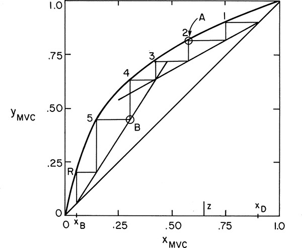
A2. For this McCabe-Thiele diagram, answer the following questions:
a. (1) What is the actual feed tray?
(2) What is the mole fraction MVC in the feed?
(3) What is the vapor composition on the feed tray?
(4) What is the liquid composition on the feed tray?
b. Is the feed a superheated vapor feed, saturated vapor feed, two-phase feed, saturated liquid feed, or subcooled liquid feed?
c. Is the temperature at stage 7 higher, lower, or the same as at stage 1?
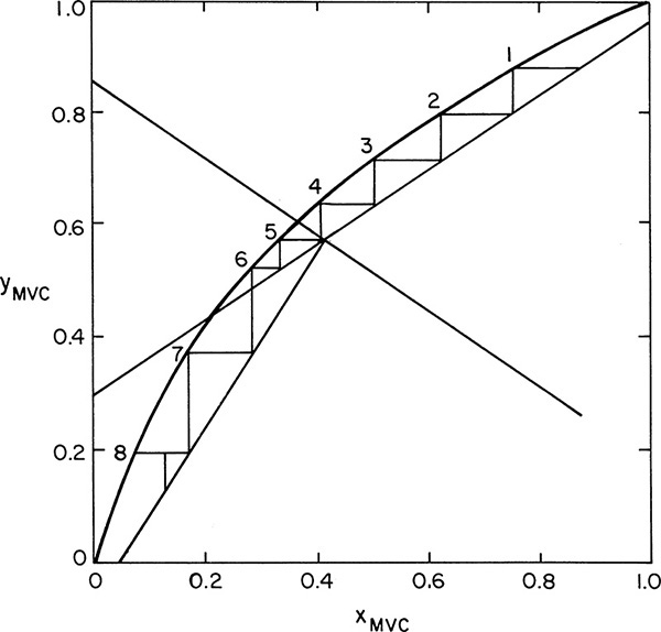
A3. Suppose that constant mass overflow is valid instead of CMO. Explain how to carry out the Lewis and McCabe-Thiele procedures in this case.
A4. Drawing the McCabe-Thiele graph as yMVC versus xMVC is traditional but not necessary. Repeat Example 4-3, but plot yw versus xw. Note the differences in the diagram. Do you expect to get the same answer?
A5. For distillation when CMO is valid, show the flow profiles schematically (plot Lj and Vj versus stage location) for
a. Subcooled liquid feed
b. Two-phase feed
c. Superheated vapor feed
A6. A distillation column is operating under a vacuum. The column has 18 stages with the feed at stage 9, a partial reboiler, and a partial condenser. The pressure drop is 5.0 mm Hg in the condenser, 4.0 mm Hg in the reboiler, and 1.0 mm Hg per stage. The pressure of the condenser is controlled at 100 mm Hg. What is the pressure of the reboiler?
A7. What is the effect of column pressure on distillation? To explore this consider pressure’s effect on the reboiler and condenser temperatures, the volumetric flow rates inside the column, and the relative volatility, which can be estimated for hydrocarbons from the DePriester charts.
A8. What happens if we try to step off stages from the top down and EMV is given? Determine how to do this calculation.
A9. When is it safe to ignore subcooling of the reflux liquid and treat the reflux as a saturated liquid? Do a few numerical calculations for either methanol and water or ethanol and water to illustrate.
A10. Eqs. (4-53) and (4-54) are mass balances on particular phases. When are these equations valid?
A11. When might you use an intermediate condenser on a column? What are the possible advantages?
A12. When would just a stripping column be used?
A13. We have a binary distillation column. The feed flow rate, F, the mole fraction MVC in the feed, z, and the initial feed temperature are constant. Column pressure, p, and distillate and bottoms mole fractions, xD and xB, are constant. Reflux is a saturated liquid, and the reflux ratio is L/D = 1.20 × (L/D)min. A heat exchanger uses waste heat, Qw, to heat the feed.
As Qw increases, does
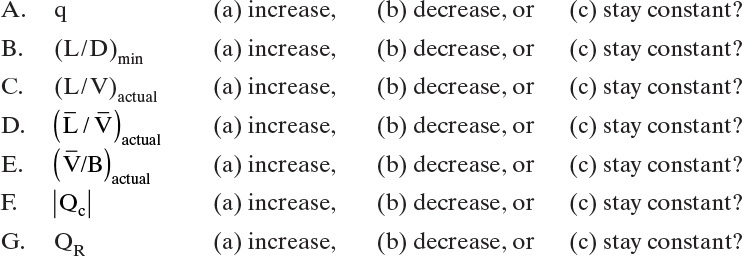
Think your way through this problem using the tools developed in this course (definition of q and feed line, mass and energy balances, and McCabe-Thiele diagrams) as reasoning tools. Hint: The parts of this problem are listed in a logical order of solution.
A14. Explain with a McCabe-Thiele diagram how changing feed temperature (or equivalently, q) may help an existing column achieve the desired product specifications.
A15. Develop a key relations chart for binary McCabe-Thiele distillation. That is, on one sheet of paper summarize everything you need to know about binary distillation. You will probably want to include information about operating lines, feed lines, efficiencies, subcooled reflux, and so forth.
B. Generation of Alternatives
B1. Invent your own problem that is distinctly different from those discussed in this chapter. Show how to solve this problem.
B2. Several ways of adapting existing columns to new uses were listed. Generate new methods that might allow existing systems to meet product specifications that could not be met without modification. Note that you can postulate a complex existing column, such as one with an intermediate reboiler.
C. Derivations
C1. For Example 4-4 (open steam) show that the x intercept (y = 0) is at x = xB.
C2. Derive the bottom operating line for a column with a total reboiler. Show that this is the same result as is obtained with a partial reboiler.
C3. Derive Eqs. (4-51) and (4-52) for side streams.
C4. For a side stream below the feed:
a. Draw a sketch corresponding to Figure 4-22A.
b. Derive the operating equation and y = x intercept.
c. Sketch the McCabe-Thiele diagram.
C5. Derive the operating equations for the two middle operating sections when an intermediate reboiler is used (see Figures 4-23A and 4-23B). Show that the operating line with slope of L′/V′ goes through the point y = x = xB.
C6. Show that the total amount of cooling needed is the same for a column with one total condenser (Qc) as for a column with a total condenser and an intermediate total condenser (Qc + QI). F, z, q, xD, xB, and QR are constant for the two cases. Sketch a system with an intermediate condenser. Derive the operating equations for the two middle operating lines, and sketch the McCabe-Thiele diagram.
C7. For the stripping column shown in Figures 4-24A and 4-24C, show formally that the intersection of the bottom operating line and the feed line is at yD. In other words solve for the intersection of these two lines.
C8. Develop the McCabe-Thiele procedure for the enriching column shown in Figure 4-24B.
C9. For Example 4-3 prove that:
a. The top operating line and the y = x line intersect at y = x = xD.
b. The bottom operating line and the y = x line intersect at y = x = xB.
C10. Derive the operating equation for section 2 of Figure 4-17. Show that the equations are equivalent whether the mass balance envelope is drawn around the top of the column or the bottom of the column.
C11. Sketch the McCabe-Thiele diagram if the Murphree liquid efficiency is constant and EML = 0.75.
C12. For a simple, single-feed distillation column derive an equation for calculation of ![]() from
from ![]() .
.
C13. Derive the equations to calculate (![]() ) when a superheated boilup is used.
) when a superheated boilup is used.
C14. Derive the equations to calculate (![]() ) when direct superheated steam is used.
) when direct superheated steam is used.
a. In a binary distillation column with two feeds, show that the intersection of the top and bottom operating lines occurs at the feed line for fictitious feed FT where FT = F1 + F2, zTFT = z1F1 + z2F2, and hF,TFT = hF,1F1 + hF,2F2.
Suggestion: Draw the McCabe-Thiele diagram for the actual column with three operating lines using both actual feed lines. On the same diagram draw the two operating lines for a column with the single mixed feed FT (they are unchanged from top and bottom operating lines of a two-feed column) and then determine the feed line for this mixed column.
b. Assuming that CMO is valid, show that qT ≈ (F1q1 + F2q2)/FT
C16. Derive Eqs. (4-56a) and (4-56b).
*Answers to problems with an asterisk are found at the back of the book.
D1. A continuous, steady-state distillation column with a total condenser and a partial reboiler is separating 100.0 kmol/h of a 55.0 mol% methanol, 45.0 mol% water feed at 1.0 atm (see Table 2-7 for data). We desire a distillate product that is 90.0 mol% methanol and a bottoms product that is 5.0 mol% methanol. Assume CMO.
a. If the external reflux ratio L/D = 1.25, plot the top operating line.
b. If the boilup ratio ![]() , plot the bottom operating line.
, plot the bottom operating line.
c. Step off stages, starting at the bottom, with the partial reboiler. Use the optimum feed stage. Report the optimum feed stage and the total number of stages.
d. Plot the feed line. Calculate its slope. Calculate q. What type of feed is this?
D2. We are separating ethanol and water. All percentages are mol%. Column pressure is at 1.0 atm. Find the q values and plot the feed lines for the following situations:
a. Feed is 60% ethanol and flashes in the column with V/F = 0.37.
b. Feed is 40% ethanol and is a two-phase mixture with liquid and vapor in equilibrium at a temperature of 84.1°C.
c. Feed is 40% ethanol and is a liquid at 20°C.
d. Feed is 40% ethanol and is a vapor at 120°C.
e. Feed is 50% ethanol and is a subcooled liquid. One mole of vapor must be condensed to heat 12 moles of feed to their boiling point.
f. Feed is 20% ethanol, and 70% is vaporized in a flash distillation system. The products of the flash system are fed separately to different feed stages. Calculate the two q values, and plot the two feed lines.
D3.*
a. A feed mixture of ethanol and water is 40.0 mol% ethanol. The feed is at 200°C and is at a high enough pressure that it is a liquid. It is input into the column through a valve, where it flashes. Column pressure is 1.0 kg/cm2. Find the slope of the feed line.
b. We are separating ethanol and water in a distillation column at a pressure of 1.0 kg/cm2. Feed is 50.0 wt% ethanol. The feed is a liquid at 250°C and flashes when the pressure is dropped as it enters the column. Find q. Data are in Figure 2-4. Assume CMO is valid.
D4.*
a. We have a superheated vapor feed of 60.0 mol% MVC at 350°C. Feed flow rate is 1000.0 kmol/h. Feed plate temperature is 50°C. For this mixture the average heat capacities are CPL = 50.0 cal/(mol°C), CPV = 25.0 cal/(mol°C); and latent heat of vaporization is λ = 5000.0 cal/mol. Plot the feed line for this feed.
b. If a feed is a two-phase feed that is 40.0 mol% vapor, find the value of q and the slope of the feed line.
c. If the feed to a column is a superheated vapor and 1 mole of liquid is vaporized on the feed plate to cool 5.0 moles of feed to a saturated vapor, what is the value of q? What is the slope of the feed line?
D5.* A distillation column is operating with subcooled reflux. The vapor streams have an enthalpy of H1 = H2 = 17,500 Btu/lbmol, while the saturated liquid h1 = 3100.0 Btu/lbmol. Enthalpy of the reflux stream is h0 = 1500.0 Btu/lbmol. The external reflux ratio is set at L0/D = 1.1. Calculate the internal reflux ratio inside the column, L1/V2.
D6. A stripping column with an additional feed is separating two feeds containing acetone and ethanol. The column has a partial reboiler and no condenser. Feed 1 is 70.0 mol% acetone, has a feed rate F1 = 200.0 kmol/h, and enters as a saturated liquid at the top of the stripping column. Feed 2 is 44.0 mol% acetone, has a flow rate F2 = 100.0 kmol/h, is a two-phase mixture that is 40.0 mol% vapor, and enters the column at its optimum feed location. Boilup ratio ![]() , and bottoms is 26.0 mol% acetone. CMO is valid. Find
, and bottoms is 26.0 mol% acetone. CMO is valid. Find
a. Distillate and bottoms flow rates, D and B, and distillate mole fraction of acetone ydist.
b. Optimum feed location for feed F2 and the total number of equilibrium stages required.
D7.* A distillation column with a total condenser is separating a feed that is 30.0 mol% acetone from ethanol. Distillate xD = 0.90 and bottoms xB = 0.13 both mole fractions acetone. Assume CMO is valid. L/V = 0.8. Boilup ratio ![]() .
.
a. Find the composition of the liquid leaving the fifth stage below the total condenser.
b. The column has a partial reboiler that acts as an equilibrium contact. Find the vapor composition leaving the second stage above the partial reboiler.
c. Find optimum feed plate location, total number of stages, and required q value of feed.
Equilibrium data for acetone (A) and ethanol at 1 atm (Perry et al., 1963, pp. 13-4) are

D8.* For Problem 4.D7c for separation of acetone from ethanol, determine
a. The number of stages required at total reflux.
b. The values of (L/V)min and (L/D)min.
c. How much larger the L/D used is than (L/D)min.
d. The number of real stages required for L/V = 0.8 if EMV = 0.75.
D9. We are separating acetone and ethanol in a distillation column with a total condenser and a partial reboiler. The column has two feeds and operates at a pressure of 1.0 atm. Feed 1 is a saturated liquid that is 60.0 mol% acetone and has a feed rate of F1 = 200.0 kmol/h. The second feed is 40.0 mol% acetone, has a feed rate of F2 = 300.0 kmol/h, and is a two-phase mixture that is 20% vapor. Assume CMO is valid. Bottoms product is 10.0 mol% acetone, and distillate product is 80.0 mol% acetone.
a. External reflux ratio L/D = 2.0. Find the number of stages required, the optimum feed stage locations, and the boilup ratio ![]() .
.
b. Find the minimum external reflux ratio (L/D)min for part a.
c. If feed 2 is changed to a superheated vapor that forces 1.0 mole of liquid to vaporize at the feed stage to cool every 5.0 moles of feed 2 to a saturated vapor, find (L/D)min. Hint: The answer is not the same as in part b.
D10.* A distillation column is separating phenol from p-cresol at 1.0 atm pressure. Distillate is 96.0 mol% phenol. An external reflux ratio of L/D = 4 is used, and reflux is returned to the column as a saturated liquid. The equilibrium data can be represented by a constant relative volatility, αphenol–cresol = 1.76 (Perry et al., 1963, pp. 13-3). CMO can be assumed.
a. What is the vapor mole fraction leaving the third equilibrium stage below the total condenser? Solve this problem using an analytical, stage-by-stage calculation alternating between the operating equation and the equilibrium equation.
b. What is liquid mole fraction leaving sixth equilibrium stage below the total condenser? Solve this problem graphically using a McCabe-Thiele diagram plotted for αp–c = 1.76.
D11. 200.0 kmol/h of a saturated vapor feed that is 16.0 mol% ethanol and 84.0 mol% water is fed to an enriching column with a partial condenser that produces a bottoms product that is 3.0 mol% ethanol. Bottoms flow rate B = 160.0 kmol/h. Reflux is a saturated liquid. P = 1.0 atm. Assume CMO is valid. Find D, L/V, L/D, yEtOh,dist, and number of equilibrium contacts required.
D12. A distillation column is connected to another separation device. The fresh feed to the column is F = 1000.0 kmol/h of a saturated vapor that is 20.0 mol% ethanol and 80.0 mol% water. The feed is input at its optimum feed stage. The distillation column has a partial condenser and no reboiler. The column is heated with direct injection of pure steam that is a saturated vapor at 1.0 atm. The ratio bottoms flow rate/steam flow rate = B/S = 5.0. The reflux ratio L0/D = 1.0. The distillate from the column is 70.0 mol% ethanol and the bottoms is 1.0 mol% ethanol. The column operates at a pressure of 1.0 atm, the reflux is returned as a saturated liquid, and CMO is assumed to be valid.
The distillate is sent to a separation device that, because it operates on a different principle than distillation, is not limited by the presence of an azeotrope. The device produces product P and recycle stream R that is a saturated liquid returned to the distillation column at its optimum feed stage. The product P concentration from the device is 98.7 mol% ethanol.
a. Find steam flow rate S, bottoms flow rate B, distillate flow rate D, product flow rate P, and recycle rate R—all in kmol/h—and find mole fraction of ethanol in recycle stream xR.
b. For the distillation column find the optimum feed plate for the recycle stream, the optimum feed plate for the fresh feed, and the total number of equilibrium stages required.
a. We have 150 kmol/h of a saturated vapor feed at 1.0 atm that is 20.0 mol% methanol and 80.0 mol% water. This feed is sent to a rectifying column equipped with a total condenser that produces 20.0 mol/h of distillate that is 90.0 mol% methanol. CMO is assumed valid, and the column is at 1.0 atm. Find B, xbot, and the number of equilibrium stages required.
b. A suggested improvement is to take a fraction of the feed, fL, condense it to a saturated liquid, and feed it higher in the column than the saturated vapor feed that enters the bottom of the rectifier. For the same problem as in part a, set fL = 0.3 so that the liquid feed rate is FL = 45.0 kmol/h and the vapor feed rate is FV = 105 kmol/h. The two feeds have the same composition (20.0 mol% methanol), but they are not in equilibrium. The column is equipped with a total condenser at the top, and it produces 20.0 mol/h of distillate that is 90.0 mol% methanol. CMO is assumed to be valid. Find B, xbot, and the number of equilibrium stages required.
c. Compare the two processes. When do you think the system in part b might be more economical?
D14. A distillation column with open steam heating is separating a feed that is 80.0 mol% methanol and 20.0 mol% water in a steady-state operation. The column has 10 stages, a total condenser, and the feed is on stage 5. Operation is at 1.0 atm. The steam is pure water and is a saturated vapor. CMO is assumed to be valid. At 2:16 a.m. 25 days ago the feed and distillate flows were shut off (D = F = 0), but the steam rate was unchanged and the total condenser is still condensing the vapor to a saturated liquid. The column has now reached a new steady-state operation.
a. What is the current methanol mole fraction in the bottoms?
b. At the new steady state estimate the methanol mole fraction in the reflux liquid leaving the total condenser.
D15. One of the old columns in your plant failed. You have been putting together a jury-rigged system to separate propane from n-butane. The column you have found is empty, so within reason you can put in as many stages as needed. It is equipped with a partial condenser and a total reboiler. The column is restricted to a maximum pressure of 800.0 kPa, which means that refrigeration is needed. You have a source of refrigeration, but output is limited to 6000.0 kW. Feed is a saturated liquid at 800.0 kPa that is 56.0 mol% propane. Unless stated otherwise distillate should be 99.9 mol% propane, and bottoms should be 1.0 mol% propane or less. You have more feed available than can be processed.
a. Generate a y-x graph at 800.0 kPa from the DePriester chart or from Table 2-3, or have Aspen Plus generate the graph. From the DePriester chart or Table 2-3 find the boiling points of propane at 800.0 kPa (set Kp = 1.0) and of n-butane at 800.0 kPa (set Kn-b = 1.0). The boiling range for the complete y-x diagram lies between these two temperatures. Pick a temperature between the two boiling points, find Kp and Kn-b, calculate xn-b = (Kp – 1)/(Kp-Kb), xp = 1 – xn-b, yp = Kpxp, and yn-b = Kn-bxn-b. Doing this for five to ten temperatures generates the y-x graph. If Table 2-3 is used, then a spreadsheet works very well.
Parts b to f can be done graphically (which is actually easier) or with Aspen Plus.
b. If you built a system with a very large number of stages (e.g., N > 100) estimate the kmol/h of 99.9 mol% distillate that can be produced and kmol/h of feed processed (bottoms ≤ 1.0 mol% propane).
c. Repeat part b for a 90.0 mol% pure propane distillate and 1% or less propane in the bottoms for a saturated liquid feed.
d. If the required purity of the bottoms stream is changed to 10.0 mol% propane, repeat part b (distillate is 99.9 mol% propane).
e. Repeat part b for a 99.9 mol% pure propane distillate and 1% or less propane in the bottoms if the feed is a saturated vapor that is 56.0 mol% propane.
f. Repeat part b for a 99.9 mol% pure propane distillate and 1% or less propane in the bottoms if the feed is a saturated liquid that is 66 mol% propane.
Data: Heat of vaporization of propane at 800.0 kPa is 18,800 kJ/kmol and for butane at 800.0 kPa is 22,600 kJ/kmol (NIST web book).
D16.* Estimate q for Problem 3.D6. Assume the feed stage is at same composition as the feed.
D17. A mixture of acetone and ethanol is fed to an enriching column. The feed flow rate is 100.0 mol/min. Feed is 60.0 mol% acetone and is a saturated vapor. A liquid side product is withdrawn from the second stage below the total condenser at a flow rate of S = 15.0 mol/min. Reflux is returned as a saturated liquid. Distillate is 90.0 mol% acetone. External reflux ratio is L/D = 7/2. Column pressure is 1.0 atm. Column is adiabatic, and CMO is valid. Find mole fraction of acetone in the sidestream xS, mole fraction of acetone in the bottoms xB, and number of equilibrium stages required. Note: Trial and error is not required.
D18. A stripping column with two feeds is separating acetone and ethanol at 1.0 atm. Feed F1 is a saturated liquid and is fed into the top of column (no condenser). Flow rate of F1 is 100.0 kmol/h, and this feed is 60.0 mol% acetone. Feed F2 is 40.0 mol% acetone, it is a two-phase feed that is 80% vapor, and flow rate is 80.0 kmol/h. Bottoms is 4.0 mol% acetone. The column has a partial reboiler.
a. Calculate ![]() .
.
b. If ![]() , find D and yD, the optimum feed stage for feed F2, and the total number of stages. Step off stages from the bottom upward.
, find D and yD, the optimum feed stage for feed F2, and the total number of stages. Step off stages from the bottom upward.
D19.* A distillation column is separating acetone and ethanol. The column effectively has six equilibrium stages plus a partial reboiler. Feed is a two-phase feed that is 40% liquid and 75.0 mol% acetone. Feed rate is 1000.0 kmol/h, and the feed stage is fourth from the top. The column is now operating at a steady state with the bottoms flow valve shut off. However, a distillate product is drawn off, and the vapor is boiled up in the reboiler. L0/D = 2. Reflux is a saturated liquid. CMO can be assumed. p = 1 atm. Equilibrium data are in Problem 4.D7. Find the distillate composition. If one drop of liquid in the reboiler is withdrawn and analyzed, predict xB.
D20.* A distillation column with a total condenser and a partial reboiler is separating ethanol and water at 1 kg/cm2 pressure. Feed is 32.0 mol% ethanol and is at 30°C. Feed flow rate is 100.0 kmol/h. The distillate product is a saturated liquid, and distillate is 80.0 mol% ethanol. The condenser removes 2,065,113 kcal/h. The bottoms is 4.0 mol% ethanol. Assume that CMO is valid. Find the number of stages and the optimum feed stage location. Data: CPL,EtOH = 24.65 cal/(mol°C) at 0°C. The enthalpy-composition diagram is given in Figure 2-4, and the y-x diagram is in Figure 2-2. Note: Watch your units.
D21. The following hybrid system shown for separating methanol and water is one way of coupling membrane separators with distillation. The gas permeation membrane separator is designed to produce yp = 60.0 mol% methanol and yr = 30.0 mol% methanol for pr = 1.0 atm and pp = 0.2 atm. The cut θ = Fp/Fin = 1/3. Assume ideal gases in the membrane separator. The feeds to the distillation column are both saturated vapors at 1.0 atm pressure at mole fractions 0.60 methanol and 0.30 methanol, respectively. Assume CMO is valid. The column has a total condenser and a partial reboiler. Distillate mole fraction is 0.9 methanol, and bottoms mole fraction is 0.05 methanol. Find:
a. The optimum feed stages and the total number of stages if L/D = 3.25.
b. (L/D)min.
Note: Parts a and b are independent of each other.
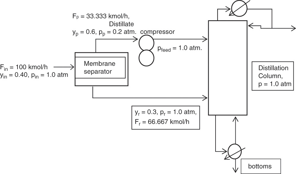
D22.* When water is the more volatile component, we do not need a condenser but can use direct cooling with boiling water. This situation was shown in Problem 3.D3. yD = 0.92, xB = 0.04, z = 0.4 (all mole fractions water), feed is a saturated vapor, feed rate is 1000 kmol/h, p = 1 atm, CMO is valid, the entering cooling water (C) is a saturated liquid and is pure water, and C/D = 3/4. Derive and plot the top operating line. Note that external balances (i.e., balances around the entire column) and equilibrium data are not required.
D23.* When water is the MVC, we do not need a condenser but can use direct cooling. This was illustrated in Problem 3.D3. We set yD = 0.999, xB = 0.04, z = 0.4 (all mole fractions water), feed is a saturated liquid, feed rate is 1000.0 kmol/h, p = 1 atm, CMO is valid, the entering cooling water (C) is pure water, and C/D = 3/4. The entering cooling water is at 100°F, and its boiling temperature is 212°F. Data: CPL,W = 18.0 BTU/(lb mol°F), MWW = 18, and λW = 17,465 Btu/lb mol. Find the slope of the top operating line, L/V. Note: Equilibrium data are not needed.
D24. A stripping column receives 100.0 kmol/h of a saturated liquid feed that is 40.0 mol% ethanol and 60.0 mol% water. The column has a partial reboiler and produces a bottoms product that is 4.0 mol% ethanol. B = 35.0 kmol/h. p = 1.0 atm. Assume CMO is valid.
a. Find D, ![]() , and yEtOh,dist.
, and yEtOh,dist.
b. Derive and plot the bottom operating line.
c. Find the number of equilibrium contacts required.
D25. We are separating methanol and water. Calculate the internal reflux ratio inside the column, L1/V2, for the following cases. The column is at 101.3 kPa. Data are available in Table 2-7 and in Problem 3.E1.
a. Distillate product is 99.9 mol% methanol. External reflux ratio is L0/D = 1.2. Reflux is cooled to 40.0°C (i.e., it is subcooled).
b. Repeat part a using a saturated liquid reflux. Compare with part a.
D26. A distillation column with a partial condenser and a total reboiler is separating two feeds of acetone and ethanol. One feed is 100.0 mol/min of 50.0 mol% acetone that is a superheated vapor where approximately 1 mole of liquid will vaporize on the feed stage for each 20.0 moles of feed. The second feed is a saturated liquid, flows at 150.0 mol/min, and is 35.0 mol% acetone. We desire a distillate product that is yD = 85.0 mol% acetone and a bottoms product that is xB = 10.0 mol% acetone. Boilup is returned as a saturated vapor. Column operates at a pressure of 1.0 atm. Assume CMO.
a. Find ![]() . (Plot both feed lines to decide which one to use.)
. (Plot both feed lines to decide which one to use.)
b. Operate at ![]() . The partial condenser is an equilibrium contact. If the stages each have a Murphree liquid efficiency of 0.75, find optimum feed locations for each feed and total number of real stages. (It is easiest to start at the top and step down.)
. The partial condenser is an equilibrium contact. If the stages each have a Murphree liquid efficiency of 0.75, find optimum feed locations for each feed and total number of real stages. (It is easiest to start at the top and step down.)
D27.* A distillation column is separating methanol from water at a pressure of 1.0 atm. The column has a total condenser and a partial reboiler. In addition a saturated vapor stream of pure steam is input on the second stage above the partial reboiler (see the following figure).
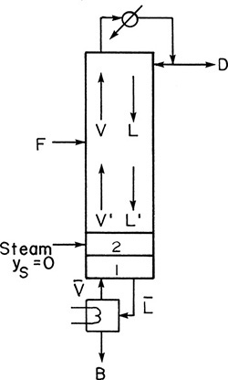
The feed flow rate is 2000.0 kmol/day. Feed is 48.0 mol% methanol and 52.0 mol% water and is a subcooled liquid. For every 4.0 moles of feed, 1.0 mole of vapor must condense inside the column. Distillate is 92.0 mol% methanol. Reflux is a saturated liquid, and L0/D = 1.0. Bottoms is 8.0 mol% methanol. Boilup ratio is ![]() . Assume that CMO is valid. Find the optimum feed plate location and the total number of equilibrium stages required.
. Assume that CMO is valid. Find the optimum feed plate location and the total number of equilibrium stages required.
D28. A stripping column is separating 10,000 mol/day of a saturated liquid feed. The column has a partial reboiler. Feed is 60.0 mol% acetone and 40.0 mol% ethanol. Bottoms product is 2.0 mol% acetone. Operate at a boilup rate ![]() . Find yD, N, D, and B.
. Find yD, N, D, and B.
D29. A distillation column uses the optimum feed stage. A liquid side stream is withdrawn on the third stage below the total condenser at a rate of 15.0 kmol/h. Feed rate is 100.0 kmol/h of a 60.0 mol% acetone and 40.0 mol% ethanol two-phase mixture that is 20% vapor. Distillate is 90.0 mol% acetone, and bottoms is 10.0 mol% acetone. We operate with an external reflux ratio of L/D = 3. A partial reboiler is used. Find mole fraction ethanol in the side stream xS, optimum feed location, and total number of equilibrium contacts needed.
D30.* A distillation column is separating methanol from water. The column has a total condenser that subcools the reflux so that 1 mole of vapor is condensed in the column for each 3 moles of reflux. L0/D = 3. A liquid side stream is withdrawn from the second stage below the condenser. This side stream is vaporized to a saturated vapor and then mixed with the feed and input on stage 4. The side withdrawal rate is S = 500.0 kmol/h. The fresh feed is a saturated vapor that is 48.0 mol% methanol. Fresh feed rate is F = 1000.0 kmol/h. A total reboiler is used, which produces a saturated vapor boilup. Distillate is 92.0 mol% methanol, and bottoms is 4.0 mol% methanol. Assume CMO. Find
a. The total number of equilibrium stages required.
b. The value of ![]() .
.
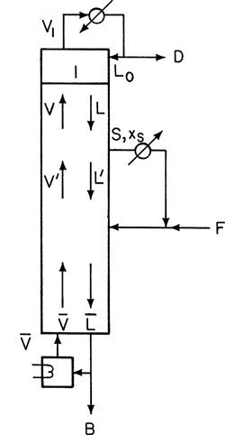
D31.* 150.0 mol/h of a saturated liquid that is 25.0 mol% ethanol and 75.0 mol% water is fed to a distillation column with a total condenser and a partial reboiler. Reflux is a saturated liquid, and CMO is valid. The column has three equilibrium stages (i.e., four equilibrium contacts), and the feed stage is second below the condenser. Bottoms is 5.0 mol% ethanol, and distillate is 63.0 mol% ethanol. Find the required external reflux ratio.
D32.* 50.0 kmol/h of a saturated liquid that is 40.0 mol% acetone and 60.0 mol% ethanol was being separated in a column at 1.0 atm. The column has a total condenser and a partial reboiler. There are eight equilibrium stages in the column, and the feed plate is the third stage above the reboiler. Three months ago the distillate flow was shut off (D = 0), but feed was continued, and the column kept running. The boilup ratio was set at the value of ![]() . Equilibrium data are given in Problem 4.D7. CMO can be assumed. What is xB?
. Equilibrium data are given in Problem 4.D7. CMO can be assumed. What is xB?
D33.* A distillation column is separating 1000.0 mol/h of a 32.0 mol% ethanol and 68.0 mol% water mixture. The feed enters as a subcooled liquid that condenses 1 mole of vapor on the feed plate for every 4.0 moles of feed. The column has a partial condenser, uses open steam heating, and is at 1.0 atm. Distillate product yD = 0.75, and bottoms product xB = 0.10. CMO is valid. The steam used is pure saturated water vapor.
a. Find the minimum external reflux ratio.
b. Using L/D = 2.0(L/D)min, find the number of real stages and the real optimum feed location if the Murphree vapor efficiency is 2/3 for all stages.
c. Find the steam flow rate used.
D34.* A distillation column with two equilibrium stages and a partial reboiler (three equilibrium contacts) is separating methanol and water. The column has a total condenser. 150.0 mol/h of feed, a 45.0 mol% methanol mixture, enters the column on the second stage below the condenser. The feed is a subcooled liquid. To heat 2.0 moles of feed to the saturated liquid temperature, 1 mole of vapor must condense at the feed stage (Note: This is an extreme amount of subcooling that would not be done in practice). Distillate is 80.0 mol% methanol. Reflux is a saturated liquid, and CMO can be assumed. An external reflux ratio of L/D = 2.0 is used. Find the resulting bottoms concentration xB. Data are in Table 2-7.
E. More Complex Problems
E1. A system called a pump-around is shown in the following figure. Saturated liquid is withdrawn from stage 2 above the partial reboiler, and the liquid is returned to stage 3 (assume it is still a saturated liquid). Pump-around rate is P = 40.0 kmol/h. The column is separating methanol and water at 101.3 kPa. The feed flow rate is 100.0 kmol/h. The saturated liquid feed is 60.0 mol% methanol. Bottoms product is 2.5 mol% methanol, and distillate product is 95.0 mol% methanol. The column has a total condenser, and the reflux is a saturated liquid. Assume CMO. Use (L/D) = 2.0 × (L/D)min. Data are given in Table 2-7. Find xp, the optimum feed stage, and the total number of equilibrium stages required.
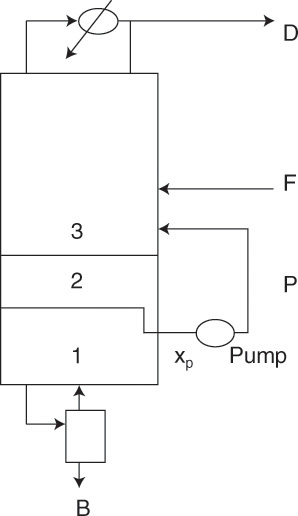
E2. A distillation column is separating 127.6 kg/min of a feed at 30°C and 130.0 kPa that is 37.6 wt% n-pentane and 64.2 wt% n-heptane. The distillation column has a total condenser and a partial reboiler. Pressure of the column at the top registers 110.0 kPa and at the bottom 120.0 kPa. At an external reflux ratio of 2.2 the distillate flow rate is measured as 48.5 kg/min of 99.8 wt% n-pentane at 39°C and the bottom is 99.92 wt% n-heptane at 128°C. The flow meter for the bottoms is broken. You have complained to the shift foreman that the mole fractions of the feed cannot be correct and at least one of the flow rates must be wrong, but he is adamant that “That’s what the instruments read.” The next shift foreman, who is a lot more helpful, corrects the feed wt% n-heptane as 62.4 wt% n-heptane, and notes that the bottom temperature reading has been erratic and that the pressure gauges all read correctly when the column was opened for cleaning 2 months ago, but he does not change the readings of the flow rates. He does give you the following cooling water information for the total condenser: Cooling water from an underground source at a flow rate of 235 gallons per minute enters at an average temperature of 16.1°C and leaves at 31.1°C. The condensed distillate liquid and reflux liquid are both at 37.5°C. The water meter was recalibrated last month, and he swears it is accurate within 1.0% or better of the actual water flow rate. Your job is to reconcile these results and come up with your best prediction of the bottoms flow rate. Note: For plant data, these numbers are not bad.
a. What is your best guess of the feed mole fraction? Briefly explain your rationale for this value.
b. Why is one (or more) of the flow rates probably incorrect? What else could be wrong?
c. What distillate, feed, and bottoms flow rates do you report to your boss, and what error bars do you use?
d. Should the pressure at the bottom of the column be greater than at the top of the column?
e. Is the temperature gauge at the top of the column probably correct or incorrect? What is your evidence?
f. Is the temperature gauge at the bottom of the column probably correct or incorrect? What is your evidence?
Conversion factors are listed in Appendix C and location of data in Appendix D at the end of the book.
E3.* A distillation column at 1.0 atm with at total condenser and a total reboiler is separating ethanol from water. Reflux is returned as a saturated liquid, and boilup is returned as a saturated vapor. Assume CMO is valid and stages are equilibrium stages. 1000.0 kmol/h of a saturated liquid feed that is 32.0 mol% ethanol is fed to the column on the optimum feed stage. Distillate is 80.0 mol% ethanol, and bottoms is 2.0 mol% ethanol. A liquid side stream is removed on the eighth stage from the top of the column at a flow rate of S = 457.3 kmol/h. This liquid is sent to an intermediate reboiler and vaporized to a saturated vapor, which is returned to the column at its optimum feed location. External reflux ratio is L0/D = 1.86. Find the optimum feed locations of the feed and of the vapor from the intermediate reboiler. Find the total number of equilibrium stages required. Be very neat!
E4. 100.0 kmol/h of a 25.0 mol% methanol and 75.0 mol% water feed is separated in a distillation column at a pressure of 1.0 atm. Feed is a subcooled liquid. To heat the feed to the boiling point, one mole of vapor condenses on the feed stage for every 10.0 moles of feed. Distillate is 90.0 mol% methanol, and bottoms is 2.5 mol% methanol. Boilup ratio = 1.0. The column is operated with two reflux streams. The reflux to the top stage has a flow rate of L0 = 21.4 kmol/h. Sufficient additional reflux (LR) is returned to stage 2 for the column to operate. Both reflux streams are saturated liquids. The column has a total condenser and a partial reboiler. Assume CMO. Equilibrium data are in Table 2-7.
a. Find D and B (distillate and bottoms flow rates).
b. Determine the reflux rate to stage 2 (LR) in kmol/h.
c. Find the optimum feed plate location and the total number of stages.
E5. 1000.0 kmol/day of a saturated liquid feed that is 30.0 mol% acetone and 70.0 mol% ethanol is fed at the optimum feed location to a column with a partial condenser and a partial reboiler. Operation is at p = 1.0 atm. Distillate is 90.0 mol% acetone, and bottoms is 10.0 mol% acetone. Boilup ratio ![]() . On the fourth stage above the partial reboiler, a vapor sidestream with flow rate S = 200.0 kmol/day is withdrawn, condensed to a saturated liquid, and returned to the column as feed at the optimum location. Assume CMO. Find the mole fraction of vapor side stream ys, optimum feed location, optimum location to input saturated liquid from intermediate condenser, and total number of equilibrium stages. Equilibrium data are in Problem 4.D7.
. On the fourth stage above the partial reboiler, a vapor sidestream with flow rate S = 200.0 kmol/day is withdrawn, condensed to a saturated liquid, and returned to the column as feed at the optimum location. Assume CMO. Find the mole fraction of vapor side stream ys, optimum feed location, optimum location to input saturated liquid from intermediate condenser, and total number of equilibrium stages. Equilibrium data are in Problem 4.D7.
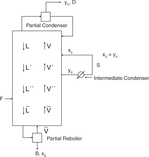
F. Problems Requiring Other Resources
F1. A distillation column separating ethanol from water uses open steam heating. The bottoms composition is 0.001 mol% ethanol. The inlet steam is pure water vapor and is superheated to 700°F. The pressure is 1.0 atm. The ratio of bottoms to steam flow rate is B/S = 2.0. Find the slope of the bottom operating line.
F2. The paper by McCabe and Thiele (1925) is a classic in chemical engineering. Read it.
a. Write a one-page critique of the paper.
b. McCabe and Thiele show a method for finding the feed lines and middle operating lines for a column with two feeds that is not illustrated here. Generalize this approach when q ≠ 1.0.
F3.* If we wish to separate the following systems by distillation, is CMO approximately valid?
a. Methanol and water
b. Isopropanol and water
c. Acetic acid and water
e. Benzene from toluene
G. Computer Simulation Problems
G1.*
a. Solve Example 4-4 with a process simulator.
b. Repeat this problem but with L/D = 1.5.
G2. Use a process simulator to find the optimum feed stage and total number of equilibrium stages for Problem 3.D6. Report the VLE correlation used. Record the values of Qcondenser and Qreboiler (in Btu/h).
G3.* Write a computer, spreadsheet, or calculator program to find the number of equilibrium stages and the optimum feed plate location for a binary distillation with a constant relative volatility. The system will have CMO, saturated liquid reflux, total condenser, and a partial reboiler. The given variables will be F, zF, q xB, xD, α, and L0/D. Test your program by solving the following problems:
a. Separation of phenol from p-cresol. F = 100, zF = 0.6, q = 0.4, xB = 0.04, xD = 0.98, α= 1.76, and L/D = 4.00.
b. Separation of benzene from toluene. F = 200, zF = 0.4, q = 1.3, xB = 0.0005, xD = 0.98, α = 2.5, and L/D = 2.00.
c. Since the relative volatility of benzene and toluene can vary from 2.61 for pure benzene to 2.315 for pure toluene, repeat part b for α = 2.315, 2.4, and 2.61.
d. Write your program so that it will calculate the fractional number of stages required. Check your program by doing a hand calculation.
H. Spreadsheet Problems
H1. (Visual Basic for Applications [VBA] required) Using the spreadsheet in Appendix B of this chapter or your own spreadsheet, solve the following problem. 250.0 kmol/h of a saturated vapor feed that is 40.0 mol% methanol and 60.0 mol% water mixture is fed to a distillation column with a total condenser and a partial reboiler. Pressure is 1.0 atm, CMO is valid, and the reflux is returned as a saturated liquid. Bottoms product is 1.1 mol% methanol, and distillate product is 99.3 mol% methanol. L/D = 4.5. Find the optimum feed stage, the total number of stages, D, and B. Use Excel to fit the equilibrium data in Table 2-7 with a sixth-order polynomial. After solving the problem, do “What if?” simulations to see what happens if the products are made purer and if L/D is decreased.
H2. (VBA required) Using the spreadsheet in this chapter’s Appendix B or your own spreadsheet, find the minimum L/D by trial and error for a saturated vapor feed of ethanol and water with z = 0.1, xD = 0.7, and xB = 0.0001.
H3. (VBA required) Either modify the spreadsheet in this chapter’s Appendix B or write a spreadsheet for binary distillation with CMO that automatically calculates (L/D)min, determines L/D = (Multiplier)(L/D)min, and then calculates the number of stages when the feed stage is specified. Use this program to find (L/D)min, the optimum feed stage, and the total number of stages for distillation of a 17.0 mol% ethanol and 83.0 mol% water feed with q = 0.5, xD = 0.7, xB = 0.0001, and Multiplier = 1.05.
Chapter 4 Appendix A. Computer Simulation of Binary Distillation
Although binary distillation problems can be done conveniently on a McCabe-Thiele diagram, simulation problems (the number of stages and feed locations are known) are easiest to solve with a computer simulator. Commercial simulators typically solve binary and multicomponent problems the same way. Although the instructions for Lab 3 discuss Aspen Plus, other simulators are similar.
Lab 3. Binary Distillation
This lab provides an opportunity to use a process simulator for binary distillation.
Goals:
• Become familiar with using RadFrac for binary distillation systems.
• Explore the effects of changing operating variables on the results of the binary distillation simulation.
• It is essential that you do the entire lab since it will help you do later labs.
Preparation:
• This lab assumes you are familiar with the previous two labs and that you are able to do basic steps with Aspen Plus.
• If you need to, use the instructions for Lab 1 as a refresher on how to use Aspen Plus.
• If problems persist while trying to run the simulations, see Appendix A at the end of the book.
I. Property Analysis
1. Start a new, blank simulation.
2. On the left side of the Navigation Pane in the All Items column, click Setup. Choose Vapor-Liquid for valid phases and no free water.
3. Either click on the blue Next button or pick from the list in the Navigation Pane what you want to do next. This set of instructions will click Next and follow the order Aspen Plus uses—that is, input properties next.
4. Aspen Plus will take you to the Component-Specifications Selection page in the Properties menu. We want to separate 1,2-dichloroethane from 1,1,2-trichloroethane. Input the components in the same way as in previous labs.
Be sure to select the correct components from the Aspen Plus menu. Note that 1,1,1-trichloroethane should not be used since it has very different properties.
5. Click on the blue Next button. Aspen Plus will take you to the Global tab of Methods-Specifications. Peng-Robinson is a reasonable VLE package. Click the Next button.
6. You should now see a popup screen titled Required Properties Input Complete. Use the default of Run Property Analysis/Setup and click OK. The screen for the control panel should tell you the steps taken by Aspen Plus. The final message should read, “Table generation completed.” (If a popup for installation of economics occurs, click Cancel.) Click the Next button. If a popup screen states, “Property analysis and setup completed successfully,” then click OK.
7. With Aspen Plus still in Properties go to the Tools tab and make sure you are in the Home tab. On the right side there is a graph icon labeled Binary. Click on this icon. You want to plot the x-y diagram from Aspen Plus for separation of 1,2-dichloroethane from 1,1,2-trichloroethane. On the binary analysis form Aspen should list your component names for these two compounds. The basis for composition should be mole fraction and vary dichloro. Ask for 100 points. Valid phases are Vapor-Liquid, pressure is 1.0 atm, and the Peng-Robinson method should be listed. Click Run Analysis. Once the T-x-y diagram appears, go to Properties→All Items list on the LHS, and under Analysis, BINRY, click Results. This gives a table that is very useful.
8. Use the table of results from Aspen Plus to calculate the relative volatility of 1,2-dichloroethane to 1,1,2-trichloroethane at 0 mol%, 50.0 mol%, and 100.0 mol% 1,2-dichloroethane, α1,2–1,1,2 = K1,2 / K1,1,2. How close is the system to a constant relative volatility = 2.24?
9. After clicking Results the items on the Tools tab in the Home tab change. On the RHS of this Tools tab, select the menu and scroll down. Select the y-x diagram. The behavior you observe on the y-x diagram is that of a system that is very close to ideal.
II. Simulation Setup:
1. We will now leave Properties. Click Simulation in the lower left of the screen. At the bottom of the flowsheet page, click the Columns tab. Use the column simulator RadFrac.
2. Draw a flowsheet of a simple column with one feed, a liquid distillate product (lower red arrow), and a liquid bottoms product. (This is the most common configuration for distillation columns.) Rename your streams. Click the arrow to the right of the RadFrac button to see alternative sketches or icons of the column. Note that picking a different icon does not change the configuration—the user has to do that in the RadFrac Specifications pages. Do not use the icon for a packed bed system as it will confuse any other users. The screen should be similar to Figure 4-A1.
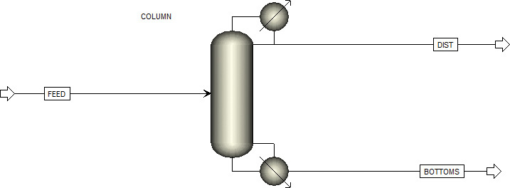
3. Make sure you are in the Home tab of the toolbar, and click the Next button. You should now have the Material Input page for your feed stream. Input the following values:
• Feed is 100.0 kmol/h
• Saturated vapor feed (vapor fraction = 1.0)
• Feed is at 1.0 atm.
• 60.0 mol% 1,2-dichloroethane and 40.0 mol% 1,1,2-trichloroethane.
• Click the Next button.
4. Aspen Plus should now show you the Specifications-Setup tab with the Configuration page for the block representing your distillation column (find this in the Navigation Pane in the All Items column on the left side of the screen). Input the following:
• The calculation type should be Equilibrium.
• For the number of stages follow Aspen Plus’s method of numbering stages (illustrated in Figure 6-2). Aspen Plus calls the condenser “stage 1” and the reboiler “stage N.” Thus if you specify N = 40, there are 38 equilibrium stages, a condenser, and a reboiler. Use N = 23 for now.
• Select Total for Condenser.
• In the Reboiler menu, select Kettle.
• Select Vapor-Liquid for Valid Phases.
• Select Standard for Convergence.
5. In the Operating Specifications there are two menus with a variety of options. For now select Distillate rate (use 60.0 kmol/h) and Reflux ratio (use 2.0). Be sure to select reflux ratio, not ![]() .
.
6. Click the Next button. If you get an error message that says you cannot have a vapor product stream with a total condenser, go back to your flowsheet, left-click on your distillate stream, right-click and select Reconnect Source, and then connect the stream to the liquid distillate product. If there are no errors, Aspen will move to the Streams tab. You need to select a feed location. Aspen Plus counts down from the top with the condenser as stage one. Input “9” and, in the Convention menu, select Vapor. In the Pressure tab it is necessary to put a pressure only for the top stage—input 1 atm. Aspen will assume you want an isobaric column and use this pressure on every stage. Ignore the Condenser and Reboiler tabs.
7. Click the Next button. A pop-up should appear that states, “Required Input Complete.” Click OK. There should be no warnings or errors. The final message should read, “Generating results.”
8. Results can be viewed by clicking on Report (in the Home tab of the menu bar) or by clicking on Results→Profiles→Stream Results→Summary in the Navigation Pane Results list on the left side of the screen. The /Simulation/Setup/Report Options/ folder is useful because it allows selection of units including mole fraction basis.
III. Simulation of 1,2-Dichloroethane and 1,1,2-Trichloroethane
In the runs that follow, if RadFrac is completed with errors, try running a similar separation that converges and then run the desired simulation again. Aspen Plus uses the previous converged run to initialize the new run. A column that will converge one time may not converge when run with different initial conditions. If the run is close to converged, the values may still be quite reasonable. You can try changing the conditions and run again. Runs with critical errors should not be used (do not look at the results, since they have no meaning). The systems for this lab were chosen so that they should converge.
When you do runs, record reflux ratio (L/D), feed rate, feed condition (fraction vaporized or temperature), the feed stage location, the number of stages (you set these values), and the following results:
• Distillate and bottoms compositions
• Temperatures of distillate and bottoms
• Maximum and minimum flow rates of liquid and vapor
• Heat loads in condenser and reboiler
Do not print out the entire Aspen Plus report!
a. We want a distillate product that is 92.0 mol% 1,2-dichloroethane and a bottoms that is 8.0 mol% 1,2-dichloroethane. Since Aspen Plus is a simulator program, it does not allow you to specify these concentrations directly. Look at the report from the previous run. If you scroll down to Mole-x-profile, the values for stage 1 (liquid leaving the condenser) are the distillate mole fractions and the values for stage 23 (liquid leaving the reboiler) are the bottoms mole fractions. Both of the purities are higher than needed.
b. First, set a distillate flow rate that will satisfy the mass balance. Find D and B from mass balances. Do this calculation accurately or you may never get the solution you want. (Hint: D = 60 is not the correct value.) Then try different columns (change number of stages and feed location) to find some that work. Use L/D = 2.0. Pick a reasonable number of stages and a reasonable feed stage (Try N = 21 and feed at 9 [vapor] to start). Simulate the column, and check the distillate and bottoms mole fractions. They should be purer than you want. Also, check the K values, and calculate the relative volatility at the top, feed stage, and bottom of the column to see how much it varies.
c. Find the optimum feed stage by trying different feed stages to see which one gives the greatest separation (highest dichloroethane mole fraction in distillate and lowest in bottoms). (Hint: Try increasing Nfeed initially.) Then decrease N (try 19, then 17) until the column no longer meets the specifications for distillate and bottoms. Now find the optimum feed stage even though you are not satisfying the specs (the optimum feed stage might satisfy the specs). Note that since the ratio of optimum feed stage to total stages is approximately constant, you probably need to check only three of four feed stages to find the optimum feed stage. If the specs are not satisfied, add back a stage and find the optimum again. If this works, you are done with this step. If the separation is better than the specs, see if you can reduce the total number of stages by one stage. If you work with a neighbor this process should not take too long. Note: Save this file for use after step d.
d. Triple the pressure of both the column and the feed, and repeat steps b and c. Determine the effect of higher pressure on the relative volatility.
e. Return to p = 1 atm and your answer for part c. Now increase the temperature of the feed instead of specifying a vapor fraction of 1. (You can find the temperature of the feed with V/F = 1 from the report for streams.) What happens?
f. Return to the simulation in part c. Determine the boilup ratio (it is given in the report for the block). Now run the simulation with this boilup ratio instead of specifying distillate rate. Then start decreasing the boilup ratio in the simulation. What happens?
g. Return to part b, but aim for a distillate product that is 99.0 mol% dichloro and a bottoms product that is 2.0 mol% dichloro. Do the mass balances (accurately), and determine settings for distillate flow rate. Try to find the N and feed location that just achieve this separation with an L/D = 2.0. Note that this separation should not be possible since the external reflux ratio (L/D) is too low. See what happens as you increase L/D (try 4 and 5). If your distillate is not at 99.0 mol% dichloro at L/D = 5, try a small decrease in your distillate flow rate.
h. Try varying different settings for Operating Specifications in the RadFrac Specifications-Setup page for the Configuration tab. For example, pick a condenser duty instead of distillate flow rate that will give the same separation.
IV. Analysis of 1,2-Dichloroethane and 1,1,1-Trichloroethane
a. Add 1,1,1-trichloroethane to your component list (click Properties, select Components in the All Items list, click on the arrow pointing toward the empty line in the component list. Add the new compound). Although not necessary, it is probably neatest and avoids possible errors if you delete 1,1,2-trichloroethane.
b. Run binary T-x-y analysis for 1,2-dichloroethane and 1,1,1-trichloroethane. Then look at the table of results, and create a y-x plot. Which compound is more volatile? Use the table of results to calculate the relative volatility of 1,1,1-trichloroethane relative to 1,2-dichloroethane α1,1,1–1,2 = K1,1,1 / K1,2 at 0 mol%, 50.0 mol%, and 100.0 mol% 1,2-dichloroethane.
c. How good is your chemistry? Can you explain the behavior you observed?
We will be using Aspen Plus simulator for multicomponent distillation calculations.
One caveat applies to Aspen Plus and all other simulators. The program can solve only the problem that you give it. If you make a mistake in the input (e.g., by not including a minor component that appears in the plant), the simulator cannot predict what will actually happen in the plant. A simulation that is correct for the problem given is not helpful if that problem does not match plant conditions. Chemical engineering judgment must always be applied when using process simulators.
Chapter 4 Appendix B. Spreadsheets for Binary Distillation
The Lewis method for binary distillation is easy to program on a spreadsheet using VBA. If you are not familiar with VBA, read Parts 1 and 2 of this appendix. If you are familiar with VBA, you can skip Part 1 and proceed to Part 2.
Appendix 4.B. Part 1. Introduction to Spreadsheets and VBA
Most engineering students are familiar with the use of spreadsheets, but they may not be familiar with the power of spreadsheets when they are coupled with VBA. VBA is an extremely useful programming language for controlling spreadsheets, Word, and other Microsoft programs, and was the most commonly recommended programming language for chemical engineers in industry (Coronell, 2005). This short introduction focuses on use of VBA for spreadsheet calculations. The particular example is binary distillation, but the VBA programming method is applicable to many of the separation methods in this book. Readers interested in more information on VBA are referred to Catapult, Inc. (1999), McFedries (2004), and Larsen (2013).
Once you have learned to program with any language (e.g., MATLAB, Mathematica, FORTRAN, C, C++) you can learn additional languages on your own. The easiest way to learn a new programming language is usually to study a few basic concepts and have available lists that delineate different programming steps, study and run a simple program that illustrates the basic features, and then create your own program by mimicking other programs. Facility comes with practice. A simple program is presented here, and other examples are in the appendices to Chapters 5, 8, 9, and 18.
VBA extends the usefulness of spreadsheets by allowing the programmer to include loops and logic decisions. Input and output is done through the spreadsheet, and the VBA editor is accessed through Excel. The examples in this book do most of the calculations in the spreadsheet to reduce the number of values that have to be transferred back-and-forth between the spreadsheet and the VBA program. The VBA program is used to update variables and for iterations, counting the number of stages or iterations, and logic decisions.
Most math symbols and functions are the same as in Excel. The basic math operations are +, –, * (multiply), /, and ^ (exponentiation). Math functions are written as Function (variable). For example, the cosine of x is written as Cos (x). Commonly used math functions are:
Abs (x) Absolute value of x
Cos (x) Cosine of x
Sin (x) Sine of x
Sqr (x) Square root of x
Log (x) Natural log of x (ln x)
Exp (x) Exponential of x (x)
VBA always determines the value on the right-hand side of equations first and then assigns this value to the left-hand side. Thus the equals sign (=) can be read as “is assigned to the value on the right hand side.” Because of this convention, equations such as x = x + 2, or x = 2x + y are perfectly valid as written and should not be simplified. Their purpose is to change the value of x.
If there is any possibility that the equation can be misread, use () to make the equation clear. For example, the equations y = a/(b + x) and y = (a/b) + x are not the same. For every left parenthesis, (, there needs to be a corresponding right parenthesis, ), to close the equation. The VBA editor tells you if this rule is violated.
VBA does loops in two different ways. For...Next loops do a set number of iterations of the loop (typically from i = 1 to a higher number [N in following loop] or a variable that is equal to a higher number). A simple loop to write values on the spreadsheet is
For i = 1 To N
Cells(7 + i, 7).Value = x
x = x + deltax
Next i
We can also write For...Next loops with a logic expression (e.g., “If eqn0 > 0, Then Exit For”) to exit the loop.
The other type of loops, Do loops, are discussed after a few introductory comments on the distillation program and in more detail by McFedries (2004). To mimic a McCabe-Thiele diagram with a spreadsheet program, we need to have an equation for the binary VLE (see Chapter 2, Appendix 2.B.1). We also need operating equations such as Eqs. (4-23) and (4-24). In addition, we need the ability to decide when to switch from one operating line to the other. This can be done by either specifying a feed stage or testing for the optimum feed stage based on passing the intersection points for xI given by Eq. (4-38a) or for yI given by Eq. (4-38b). If stepping off stages up the column, a convenient test is that the stage where yMVC first becomes greater than yI is the optimum feed stage. Finally, we need a test for when the calculation if finished. Stepping off stages up the column, the number of stages is sufficient when y > xD (or y > yD with a partial condenser), and stepping off stages down the column, the number of stages is sufficient when x < xB.
The use of a Do loop is illustrated for the case with a specified feed stage, and we are stepping off stages from the bottom up (partial reboiler is stage 1). After initializing i = 1 and x = xB, we can set up a loop to step off stages in the stripping section:
Do
y = a6*x^6+a5*x^5+a4*x^4+a3*x^3+a2*x^2+a1*x+a0
i = i + 1
x = (y/LbaroverVbar)+(LbaroverVbar-1)*xb/LbaroverVbar
Loop While i < feedstage
This loop starts with the word Do, calculates y1 from the equilibrium expression (fit to a sixth-order polynomial) at the known value of x1, and then calculates x2 from the operating equation [Eq. (4-24) solved for x] with the known value of y1. This process is repeated to calculate y2 and x3, and so forth, as long as i < the specified feed stage. When i = the feed stage we skip the loop and calculate the steps in the enriching section using another loop. Note that Do loops always end with the word Loop either by itself (see next example) or with a logic statement, as shown previously.
Do While y < xd
y = a6*x^6+a5*x^5+a4*x^4+a3*x^3+a2*x^2+a1*x+a0
i = i + 1
x = (y/LoverV)-(1-LoverV)*xd/LoverV
Loop
Note that when we enter this loop, we have just calculated the value of x on the feed stage. Thus the first value calculated is the y value leaving the feed stage.
These loops illustrate two different types of Do loops. In the first example the logic test (While i < feedstage) is done at the end of the loop, and in the second example the logic test (the While statement) is done at the beginning of the loop. We could have written the stripping and enriching section equations with either type of loop. The difference is that if the logic test is at the end of the loop, the loop will run at least the first time (e.g., if the reboiler is the feed stage).
Appendix 4.B. Part 2. Example: Binary Distillation Spreadsheet
In this section we look at a program for binary distillation to help make these statements concrete.
First, since VBA is a macro, you must enable macros.
The spreadsheet with equations and numerical results is shown in Figure 4-B1. The problem solved in the figure is to separate 1000.0 kmol/h of a saturated liquid feed that is 10.0 mol% ethanol and 90.0 mol% water. The column has a total condenser and a partial reboiler. We desire a distillate that is yD = 78.0 mol% ethanol and a bottoms that is xB = 0.06 mol% ethanol. Operation is with L/D = 2.0, and stage 7 (reboiler = 1) is the feed. CMO is assumed. Before stepping off stages the spreadsheet calculates L/V = 0.66667 (cell B8), D = 127.53, B = 872.47, and ![]() . For each stage y is calculated from equilibrium with the constants for ethanol-water in form y = f(x) (sixth-order polynomial) obtained in Eq. (2.B-1). The results are given in row 15 and following rows. To try another feed stage the value in cell H2 is changed and the VBA program is run again
. For each stage y is calculated from equilibrium with the constants for ethanol-water in form y = f(x) (sixth-order polynomial) obtained in Eq. (2.B-1). The results are given in row 15 and following rows. To try another feed stage the value in cell H2 is changed and the VBA program is run again
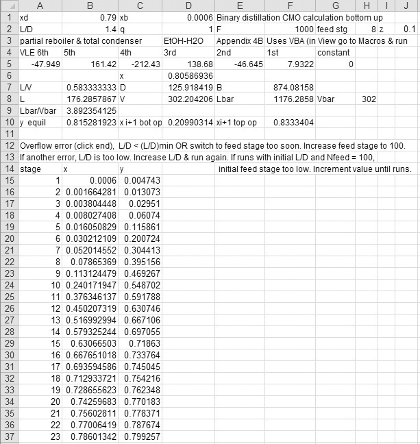
The VBA program for this spreadsheet is shown in Table 4-B1. The program starts with the Sub McCabeThstages() statement. In this statement the programmer chooses the title (McCabeThstages) with no spaces. Note that lines beginning with an ‘are comments and are ignored by the program. The statement Sheets("Sheet1").Select tells VBA where to find the spreadsheet, and the Range("A8", "G1008").Clear statement removes old results. The Dim...As Integer and Dim...As Single statements declare all variables used in the program. Data are input with statements such as xd = Cells(1, 6).Value that tell VBA that xd has value in cell (1,6) of the spreadsheet. For this example, that value is 0.78. VBA transfers values to the spreadsheet with statements such as Cells(6, 4).Value = x. The last line of the VBA program must be the End Sub statement.
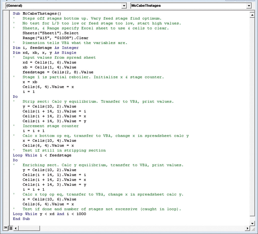
Note: Since this spreadsheet uses a VBA program, changing a value of the input in the spreadsheet (e.g., z) does not change the spreadsheet. You must also run the VBA program by doing the following steps from the spreadsheet tool bar in Excel 2007: View→Macros→View Macros and then click Run (if you want to see the VBA program, click Edit).
Note that the result is quite sensitive to the equilibrium expression used.
By varying the feed stage location, the optimum location (stage 7) can easily be found. The minimum external reflux ratio can be determined quickly by trial and error (see Problem 4.H2). The program can also be coded to find either of these values automatically (see Problems 4.H1 and 4.H3).
Obviously this problem can be solved graphically. The problem can also be solved with a hand calculation on a spreadsheet without using VBA by writing the equilibrium and operating equations in cell form and then repeating them as needed. The advantages of a programmed spreadsheet or other software tools (e.g., Binous, 2008) are a huge number of trials can be done by changing just one number (e.g., z or L/D), different systems can easily be studied by using different values for the VLE coefficients, and you do not have to manually step off 15 stages. For a single use, graphical or hand calculation with a spreadsheet may take less time. However, for multiple uses the programmed spreadsheet is obviously preferable. In all cases if the CMO assumption is not valid, the results will be incorrect. Note that this program, and all other software packages, must be checked to make sure it is producing correct results (Shacham et al., 2008).
The only logic tests included are for the feed stage location and whether the distillate mole fraction has been reached. To create a more robust program, we could check for two additional conditions. Stepping off stages up the column, the specified feed stage may be too low. In this case the x value will eventually become negative (try this on a McCabe-Thiele diagram). We can test for this occurrence by adding the following lines after the calculation of x in the enriching section loop.
If x < 0 Then
Cells(i + 7, 4).Value = "Feed stage too low"
Exit Do
End If
The person running the spreadsheet should then realize that a higher feed stage location needs to be specified.
The second condition we want to test for is a reflux ratio that is too low. If we assume that the pinch is at the feed stage, a reflux ratio that is too low will cause the intersection of the two operating lines to be above the equilibrium curve. At the intersection point, the values of xint and yint can be calculated from Eq. (4-38). The vapor equilibrium value yeq can be determined from the polynomial fit to the VLE data at x = xint. Then the following test is inserted into both stripping and enriching section loops.
If yeq < yint Then
Cells(i + 7, 3).Value = "Reflux rate too low"
Exit Do
End If
Every time you add any tests with new variables, you need to remember to include the variables in the appropriate dimension Dim statements (see Table 4-B1).