15	Expert Systems Application for the Reconfiguration of Electric Distribution Systems
	Tovar-Hernández Horacio and Gutierrez-Alcaraz Guillermo

CONTENTS

15.1  Introduction

15.2  Expert System

15.2.1  Optimal Power Flow

15.2.2  Volt/VAr Control

15.3  Case Study

15.3.1  Scenario 1

15.3.2  Scenario 2

15.3.3  Scenario 3

15.4  Summary

References

15.1  INTRODUCTION

In the past three decades, intensive effort has been devoted to formulating and solving distribution network optimal planning and operating problems. Nowadays, advances in communication and computer technologies have made feasible the development of more sophisticated methodologies to solve some of the particular problems deriving from those two general challenges. For example, in an operational framework, advances in distribution automation (DA) technology have substantially improved control and management capabilities, so that it is possible to reconfigure distribution electric systems directly from an operation control center [1]. Also, time-varying consumer demand, always an issue, can be addressed by very specific feeder reconfiguration to enable load transfers from heavy or overloaded feeders to feeders with available load capacity [2].

The concept of the smart grid is based on a distribution management system (DMS) comprising a set of hardware and software applications installed in a control center for monitoring and controlling distribution systems with a high degree of automation. An important objective is to enhance system operation efficiency and reliability. For this purpose, many utilities rely on two-way communications to monitor and control equipment at distribution substations and feeders. A DMS incorporates the measurement data from DA and advanced metering infrastructure to provide more precise load estimations of feeder sections for integrated Volt/VAr and service restoration controls [3]. The DMS, which is able to maintain information about the current and past topologies of the electric distribution system, facilitates and automates the creation of switching orders for planned and unplanned work that operators or field personnel can execute according to traditional procedures, or that can be executed automatically [1].

The software infrastructure associated with a DMS can be classified into the sets of basic or conventional applications, and advanced or intelligent applications. The former set includes conventional algorithms such as load flows, short-circuit analysis, state estimation, and load forecasting, while the latter combines these applications with database and operational criteria management to help operators to obtain the optimal operational set points of each network component [4]. The DMS is superior to older technology in terms of flexibility and handling operation planning horizons by acquiring, filtering, and manipulating data for efficient decision making. Within this environment, operators are able to determine the optimal state of the distribution system as much as an hour in advance [2].

Distribution systems are subject to operational changes that can be either smooth or critical, depending on the magnitude of the perturbation experienced. If load variations or less severe failures occur, resulting in some overloads or voltages out of limits, then a transition from the normal to the emergency state occurs, and some corrective actions can be performed to restore the system to a normal operational state. A different situation occurs when a perturbation is a permanent failure; in this case, the distribution system moves from normal to an emergency state, in which fault-clearing actions are carried out and some subsequent restorative actions can be performed to take the distribution system to a new normal operational state. These processes are illustrated in Figure 15.1.

In the normal state, relatively small or smooth changes occur, for example, hourly variations of load, and normal-state operational conditions may vary. Therefore, operators can make some decisions to take the distribution system from a nonoptimal operational condition to a better operational state by using a short-term operation planning process comprising the following strategies [4]:

FIGURE 15.1 Operational states, transitions between them, and remedial actions in electrical distribution systems.

1.  Detection of restriction violations

2.  Corrective action planning

3.  Maintenance outage programming

4.  Loss reduction by reconfigurations

5.  Volt/VAr control

A combination of these strategies allows the development of sophisticated methodologies with the capacity to obtain an optimal operative state. For example, loss reduction can be optimized by reconfiguration and Volt/VAr control.

Under the smart grid framework, a great number of algorithms and methodologies have been developed to optimize distribution system operations. In particular, solving the problem of loss minimization is a key factor in laying out circuits as well as predicting a desired system configuration for different normal-operation or contingency cases. For example, many proposals solve the reconfiguration problem from a normal-operation condition perspective involving either one or several load scenarios in order to follow load variations more accurately and to obtain minimum distribution losses for each load scenario [5]. Both of these approaches normally change the open/closed status of tie switches in a progressive manner, until they find a radial configuration of the distribution system with minimum losses, while keeping nodal voltages within limits and avoiding overloads on each feeder section, including substation transformers. In some cases, such proposals are based on conventional power flow solvers combined with topological search algorithms [6]; in others, they are based on evolutionary programming techniques, including power flow solvers [7,8] and sometimes topological search methods [9].

Nevertheless, solving the more complex problem of reconfiguration with Volt/VAr control has not been addressed with the same interest, even though its solution should result in a greater reduction of distribution losses while still maintaining better nodal voltage profiles. It has been proposed to solve this problem by multiobjective/multistep evolutionary programming techniques [9,10,11] or optimal power flow (OPF) Benders decomposition algorithms [12,13], both including the radial-structure restriction.

Furthermore, expert systems (ESs) have been shown to be useful for dealing with distribution system operation. ESs have been developed as decision-making support methodologies for distribution system operators to solve problems of restoration, feeder load balancing, voltage control, and loss minimization in distribution systems [14,15]. These tools make use of computational algorithms such as load flow, topological search, sensitivities, and optimization techniques, in order to obtain solutions that are feasible and optimal in some sense to the system operator [16]. This combination of artificial intelligence tools and numerical algorithms evolves into methodologies that could be more efficient than those based only on very complex numerical algorithms or evolutionary multiobjective methodologies for solving mixed-integer nonlinear programming [17]. In many cases, however, ESs lack solid mathematical foundations, so there is no guarantee that they reach an optimal solution; rather, it may be only a good approximation [16]. Nevertheless, due to the discrete nature of tie switching, transformer and regulator tap adjustment, and capacitor bank commutation, the solutions obtained with ESs and those based on optimization algorithms or evolutionary programming will be very similar in practical terms.

In this chapter, we propose an ES for optimal loss reduction that uses a coordinated application for reconfiguration and Volt/VAr control in the distribution system. For this purpose, the ES improves a set of solutions proposed by an OPF-based reconfiguration algorithm, executing reactive power control actions by capacitor bank commutations and regulator tap adjustments.

15.2  EXPERT SYSTEM

As mentioned, intelligent methodologies are needed to support operational decision making in an information-rich environment. In a dynamic electrical distribution system, the system operator must make decisions in real time to maintain the distribution system in an optimal operational state. ESs, or knowledge-based systems, were developed approximately 30 years ago to assist system operators in defining appropriate control actions to keep transmission or distribution systems operating under security restrictions [14,16]. Some ESs have been designed as aids for transmission and distribution system operators for voltage and reactive power control. In general, ES applications in electrical engineering are designed as knowledge-based systems based on heuristics and numerical calculations that give more intelligent solutions to complex problems than those given by conventional algorithms [16].

Our proposed ES is a rule-based system with a forward-chaining reasoning that involves two general stages: (1) finding one set of distribution system reconfigurations with voltages within limits and no overloads by means of an OPF, and (2) performing a reactive Volt/VAr control to reduce losses given by the set of reconfigurations found in stage (1).

We organized the If-Then rules into steps for making orderly and efficient decisions. In our hypothetical real-time environment where the ES must be able to act for the next load scenario, each step represents a level of the following solution process:

Step 1. Identify the actual state of switches between feeders, capacitor banks, and nodal loads for the current hour, defined as h-1.

Step 2. For the next load demand scenario, D(h), find all n options for reconfiguration and classify the options as feasible reconfigurations (FRs). Calculate each FR by the OPF algorithm, setting all capacitor banks in a disconnected state, so that each FR found does not present overloads or voltage deviations out of limits. If n = 0, the ES modifies the voltage limits until the OPF finds at least one FR.

Step 3. For each FR, perform a reactive power control by means of capacitor bank commutations to investigate their impact over distribution losses until there is no capacitor bank commutation that reduces losses.

Step 4. Find the reconfiguration with the minimum distribution losses, and name it as the new operating state, E^(h).

Step 5. Verify that E^(h) ≠ E^(h-1). If true, define the changes needed in switches and capacitor banks to pass from the E^(h-1) state to the E^(h) state, and convey this information to the system operator.

15.2.1  OPTIMAL POWER FLOW

The OPF algorithm obtains reconfigurations with voltages remaining within certain limits [12,13,18]. However, at this stage the solutions of the OPF are allowed to present slight voltage deviations out of limits, which can be corrected by reactive power/voltage control by capacitor bank switching and adjusting regulator taps. Interfaces between transmission and distribution are treated as a voltage-controlled node with one generator. These generators will have the same cost production function, such that the power sharing among them is not influenced by the most economical generation contribution, but by the least generation needed to satisfy all the loads connected to the distribution system. Hence, OPF solves an economical dispatch for each configuration r ∈ R, where R is the set of all possible radial network reconfigurations. Each reconfiguration r without overloads and voltages out of limits is included in a subset of FRs. Mathematically, the OPF can be formulated as a nonlinear optimization problem:

$\underset{\left\{P_{gi}\right\}}{\text{Min}}{C}_T\left(r\right)={\displaystyle \sum _{i=1}^{ng}\left(d_i+e{}_i{P}_{gi}+f_{i}P{g}_i^2\right)}$

(15.1)

$S\cdot toP{g}_k\left(r\right)-P{d}_k\left(r\right)={\displaystyle \sum _{j=1}^N\left|V_k\right|\left|V_j\right|\left(G_{kj}\cos \left({\text{θ}}_k-{\text{θ}}_j\right)+B_{kj}\sin \left({\text{θ}}_k-{\text{θ}}_j\right)\right)\forall k\in N}$

(15.2)

$Q{g}_k\left(r\right)-Q{d}_k\left(r\right)={\displaystyle \sum _{j=1}^N\left|V_k\right|\left|V_j\right|\left(G_{kj}\sin \left({\text{θ}}_k-{\text{θ}}_j\right)-B_{kj}\cos \left({\text{θ}}_k-{\text{θ}}_j\right)\right)\forall k\in N}$

15.3)

${\displaystyle \sum _{k\in K_{out}}{S}_{pk}\left(r\right)\le S_p^{\text{Max}}}\forall p\in Nt$

15.4

${\displaystyle \sum _{k\in K_{out}}{S}_{pk}\left(r\right)\le S_p^{\text{Min}}}\forall p\in Nts$

(15.5)

$\left|V_k^{\text{Min}}\right|\le \left|V_{k,r}\right|\le \left|V_k^{\text{Max}}\right|$

(15.6)

$S_{j,r}\le S_j^{\text{Max}}j\in Nb$

(15.7)

$Nrs=N-ng$

(15.8)

where:

N	is the total number of nodes
Nb	is the total number of branches
Nt	is the set of all substation transformers
Kout	is the set of feeders receiving power from transformer p
Spk	is the power flowing from transformer p to feeder k
$S_p^{\text{Max}}$	is the rating of transformer p
θk	is the voltage angle at node k
Pdk	is the active load at node k
Qdk	is the reactive load at node k
Pgk	is the active power injected at node k
Qgk	is the reactive power injected at node k
∣Vk∣	is the voltage magnitude at node k
$\left|V_k^{\text{Min}}\right|,\left|V_k^{\text{Max}}\right|$	are the allowed minimum and maximum voltage magnitude at node k
Sj	is the loading of feeder j
$S_j^{\text{Max}}$	is the rating of feeder j
di, ei, and fi	are the production cost factors
Gkj and Bkj	are the real and imaginary parts of the admittance matrix element Ykj, respectively
ng	is the total number of substations or generators

The objective function (Equation 15.1) is the minimization of the production cost of power provided by the utility. Constraints 15.2 and 15.3 represent the nodal power balance equations. Constraints 15.4 and 15.5 represent the maximum and minimum power output limits of the substation or generator, respectively. Inequality constraints 15.6 and 15.7 are the system operative and security constraints (upper and lower bounds), respectively [13]. Restriction 15.8 is related to the radial structure of the distribution system, where Nrs is the number of branches included in the spanning tree representing each one of the possible distribution system reconfigurations [2].

In our formulation, the OPF does not perform reactive power control to minimize distribution losses, chiefly because this process is carried out by capacitor bank switching and regulator tap adjustments, which are discrete control actions, and the OPF algorithm would have to solve a more complex mixed nonlinear and integer programming problem. Traditionally, reactive power dispatch for transmission systems has been formulated assuming that these devices are continuous variables in the OPF formulation. However, commercial capacitor bank capacities are relatively large (e.g., 300 kVAr modules), so that modeling them as continuous variables in OPF for distribution systems would lead to impractical results.

15.2.2  VOLT/VAR CONTROL

Traditionally, reactive power control is performed to minimize losses and control voltages through capacitor bank switching and regulator tap adjustments. The resulting operational state of these devices is maintained during a long period of time defined by considerable changes in seasonal load patterns. Capacitor bank switching can be fixed or commutable. In the latter case, commutation is made by local criteria such as temperature changes, low voltage, and so on. Furthermore, regulator taps are adjusted by measuring the voltage on a specific distribution node. However, under the smart grid paradigm, it is assumed that the control center must monitor and control these devices by considering their benefit to the entire distribution system, that is, minimization of loss and voltage deviation.

Capacitor bank commutations and regulator tap adjustments should strictly be modeled as discrete events. To find the best combination of capacitor bank commutations and regulator adjustments to reduce the distribution losses to a minimum, the ES performs a dynamic programming process. Experimental results show that a good practice is first to analyze the effect of capacitor banks, and then realize the tap adjustments in regulators, because capacitor banks have a great impact on loss reduction, while regulator taps have a minor effect, but can be used to make final changes in voltage magnitudes, which also help to diminish losses.

In particular, for our proposed computational methodology, we consider that capacitor banks have a modular capacity based on 300 kVAr blocks. Once the OPF has obtained the subset of FRs, the ES performs the Volt/VAr control following the next steps:

1.  Select an FR from the subset FR.

2.  For the capacitor bank set, select one capacitor block and switch it in or out, depending on its actual state. Observe its impact on distribution losses; if they augment, leave this capacitor bank in its actual state; if they drop, add the capacitor block commutation to a feasible control action (FCA) list and turn back the capacitor block to its original status. To avoid capacitor bank commutations with an almost null impact on loss reduction, it is convenient to establish a threshold value, for example, 5 kW.

3.  If there are more capacitor bank blocks to investigate, go back to Step 2. If not, go to next step.

4.  If the FCA is empty, go to Step 6. If not, go to the next step.

5.  Order the control actions in the FCA from greater to lesser impact. Once the FCA has been ordered, the control action that causes the greatest loss reduction is put into a selected control action (SCA) list.

6.  For each regulator, investigate adjustments in its tap, which can reduce the distribution loss value reached in Step 2. Select the adjustment with the greatest loss reduction, and add it to the SCA list. To avoid regulator tap adjustments with an almost null impact on loss reduction, it is convenient to establish a threshold value, for example, 5 kW.

7.  Return to Step 1 if there are more FRs to investigate. If not, create the definitive control action (DCA) list and end the process. The final DCA list will be the SCA list corresponding to the least-loss reconfiguration.

The process with OPF and Volt/VAr control, as described above, is designed for a load demand scenario h. If there are more scenarios to be analyzed, then h and h–1 are updated, and the whole process is repeated until all the load scenarios have been analyzed.

15.3  CASE STUDY

A practical distribution network with two contiguous substations is used to illustrate the ES functioning. It is considered that the distribution system operates under three-phase balanced conditions; therefore, the positive sequence network represents the system network. The complete network data are given in [17], and the corresponding single-line diagram is depicted in Figure 15.2. Both substations operate independently as radial feeders, but they can be interconnected by one of the normally open tie-line switches.

Optimal network configuration problem is solved by brute force combined with graph theory implemented in MATLAB^®. For illustrative purposes, only switches connecting tie-lines are considered for load transfer (S84, S85, S87, S88, and S91). However, to preserve a radial structure, when switch S91 operates, switch S21 or switch S83 should operate simultaneously, depending on where the load transfer takes place; switches S5, S7, S11, S12, S55, S64, S72, and S76 are in the same situation. Intra-area switches, for example, switches 89 and 97, are mainly used to achieve load balancing between feeders belonging to a substation, depending on the diversity and amount of each feeder demand. Under this consideration, it is possible to operate 15 switches and generate 32,768 possible reconfigurations. A subset of this large number of possible reconfigurations will be feasible and the rest will not be feasible due to overloads, out-of-limit voltages, or both. Table 15.1 shows individual switch operation states for 11 possible reconfigurations, which were selected randomly, the only purpose being to show how our proposal works. However, in a real-life environment, there should be an algorithm that helps to find the more promising subset of FRs.

Table 15.2 shows the location and capacity of capacitor banks; they can be connected or disconnected by 300 kVAr blocks. In this case study, regulators do not exist in the distribution system, and thus they are not included in the reconfiguration process.

Also, it is assumed that the ES acts to propose a new reconfiguration depending on the load scenario for the next hour, while taking the current scenario into account. For illustration purposes, we analyze three of the hourly load scenarios that could occur during a period of time, namely, a day ahead.

To initiate the ES process, we consider that the distribution system is operating under the reconfiguration 00 shown in Table 15.1, and the nine capacitor banks of Table 15.2 are disconnected. Additionally, voltage limits are specified as 0.95 and 1.05 p.u. in all nodes, and we will assume that all feeder sections have the very high overload limit of 100 MVA.

15.3.1  SCENARIO 1

Scenario 1 presents the loads shown in Table 15.3, for all the nodes of the distribution system. The substation voltages are set to 1.01 p.u. The five general steps are developed below:

Step 1.  The ES identifies the actual operation state E⁽⁰⁾ based on the information presented in Tables 15.1 through 15.3, also considering that the distribution system operates under the 00 reconfiguration, and all capacitor banks are disconnected.

Step 2.  The OPF obtains FRs observing overloads and voltages for the 11 reconfigurations. For scenario 1, reconfigurations 01, 09, and 10 are classified as unfeasible, while reconfigurations 00, 02, 03, 04, 05, 06, 07, and 08 are classified as feasible, that is, they are included in the subset FR.

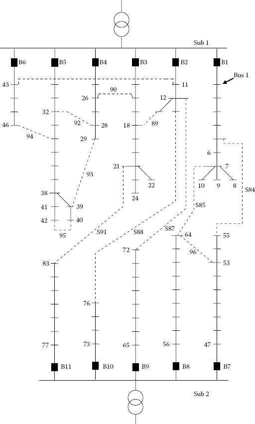
FIGURE 15.2 Distribution system with two substations and 11 feeders operating in radial structure.

TABLE 15.1
Individual Tie-Line Switch States for the 11 Possible Configurations

TABLE 15.2
Capacitor Bank Location and Capacity (kVAr)

No.	Node	Capacity
1	6	2400
2	21	2100
3	28	2400
4	37	1800
5	51	2100
6	63	1500
7	71	2400
8	75	2400
9	81	2400

TABLE 15.3
Active and Reactive Nodal Demands for Scenario 1

Step 3.  With the results of Step 2, the ES performs the reactive power control to minimize distribution losses with the connection of 300 kVAr capacitor bank blocks for each of the FRs of scenario 1. Once the ES has found all the capacitor bank blocks that should be connected in order to reduce the distribution losses to a minimal value, it goes to the next step.

Step 4.  Distribution losses for all FRs and the corresponding order with and without reactive control are shown in Table 15.4. Based on this information, the ES defines 07 as the best reconfiguration, because it has the minimum distribution losses.

The results from this table show the different order before and after applying the reactive power control; this strategy, performed by the ES to minimize losses, holds promise for helping distribution companies to achieve substantial savings, as is evident from the columns without and with reactive power control.

Step 5.  The ES finds the control actions to be performed to reach the new operating state E⁽¹⁾. The initial and final network configurations are configuration 00 and configuration 07, respectively.

It can be seen that the only changes needed to pass from the actual reconfiguration to the new one are the following:

Control action 1: Close switch S88

Control action 2: Open switch S12

Note that the control action to close tie-line switch S88 is executed first, in order to prevent the isolation of some portion of the electrical network. Since we assumed that capacitor banks were initially in disconnected status, they are connected as specified by the next control actions:

Control action 3: Connect 1200 kVAr at node 6

Control action 4: Connect 1200 kVAr at node 21

TABLE 15.4
Distribution Losses for All FRs of Scenario 1

	Without Reactive Power Control		With Reactive Power Control
Reconfiguration	Losses (MW)	Ordering	Losses (MW)	Ordering
00	0.3952	4	0.3005	5
02	0.4010	7	0.3040	6
03	0.3930	2	0.2995	3
04	0.4065	8	0.3081	8
05	0.3956	5	0.2993	2
06	0.3921	1	0.2997	4
07	0.3949	3	0.2943	1
08	0.3984	6	0.3042	7

Control action 5: Connect 1500 kVAr at node 28

Control action 6: Connect 900 kVAr at node 37

Control action 7: Connect 1200 kVAr at node 51

Control action 8: Connect 1200 kVAr at node 63

Control action 9: Connect 1500 kVAr at node 71

Control action 10: Connect 1500 kVAr at node 75

Control action 11: Connect 1500 kVAr at node 81

In this case, the control action order to connect capacitor bank blocks has been established according to Table 15.2, because no capacitor-connection sequence will cause overloads or voltages out of limits, and the final result of realizing control actions 4–11 will be the same independently of the execution order.

Note that there are many control actions for reaching the optimal reconfiguration. However, when there are small changes in reconfiguration between scenarios, the control actions will be few, mainly because we already have an optimal solution, as will be observed when scenario 2 is analyzed.

15.3.2  SCENARIO 2

The loads of scenario 2 are obtained by multiplying the active and reactive loads of scenario 1 by 1.125. Once again, the substation voltages are set to 1.01 p.u. The ES carries out Step 1 considering scenario 2, actual reconfiguration 07, and the corresponding capacitor bank status shown through the control actions 3–11 listed above.

The results of Step 2 show that reconfigurations 01, 02, 04, 09, and 10 are now unfeasible, while 00, 03, 05, 06, 07, and 08 are feasible. Application of Steps 3 and 4 produces the results shown in Table 15.5, where minimum losses are reached once again for reconfiguration 07, and the three capacitor bank control actions.

For Step 5, the ES displays the next control actions, which are the only changes with respect to the operational state E⁽¹⁾ for reaching E⁽²⁾:

Control action 1: Connect 300 kVAr at node 28

Control action 2: Connect 300 kVAr at node 37

Control action 3: Connect 300 kVAr at node 81

TABLE 15.5
Distribution Losses for All FRs of Scenario 2

According to these results, capacitor banks should be connected with the capacity listed below:

Node 6: 1200 kVAr

Node 21: 1200 kVAr

Node 28: 1800 kVAr

Node 37: 1200 kVAr

Node 51: 1200 kVAr

Node 63: 1200 kVAr

Node 71: 1500 kVAr

Node 75: 1500 kVAr

Node 81: 1800 kVAr

15.3.3  SCENARIO 3

The loads for scenario 3 are obtained by multiplying the loads of scenario 1 by 1.25 and substituting the loads at nodes 73, 74, 75, and 76 with the values of (0.8,0.2), (0.5,0.12), (2.0,1.35), and (0.9,0.38), MW and MVAr, respectively. In this case, substation voltages are set to 1.02 p.u.

For the realization of Step 1, E⁽²⁾ is taken as the actual operational state, but considering the corresponding loads of scenario 3.

The results of Step 2 show that feasible and unfeasible reconfigurations are the same as for scenario 2. Table 15.6 shows the solutions obtained by the ES after carrying out Steps 3 and 4. It is clear that now the reconfiguration 03 is the new configuration for scenario 3.

For scenario 3, the control actions displayed by the ES to the distribution system operator would be the following:

Control action 1: Close switch S12

Control action 2: Close switch S85

Control action 3: Open switch S88

Control action 4: Open switch S7

Control action 5: Disconnect 300 kVAr at node 6

Control action 6: Connect 300 kVAr at node 21

Control action 7: Connect 300 kVAr at node 28

TABLE 15.6
Distribution Losses for All Reconfigurations of Scenario 3

Control action 8: Connect 300 kVAr at node 51

Control action 9: Connect 600 kVAr at node 63

Control action 10: Connect 300 kVAr at node 71

Control action 11: Connect 600 kVAr at node 75

Control actions 1–4 are executed to change from reconfiguration 07 to 03. Control action 5 shows that the disconnection of a 300 kVAr capacitor bank block should take place, while control actions 6–11 indicate the connection of 300 or 600 kVAr capacitor bank blocks relative to their status in scenario 2. This result appears to be because the load of scenario 3 is greater than the load of scenarios 1 and 2. The final connection statuses of the capacitor banks are:

Node 6: 900 kVAr

Node 21: 1500 kVAr

Node 28: 2100 kVAr

Node 37: 1200 kVAr

Node 51: 1500 kVAr

Node 63: 1800 kVAr

Node 71: 1800 kVAr

Node 75: 1800 kVAr

Node 81: 1800 kVAr

15.4  SUMMARY

According to the results shown in this chapter, it is clear that considering only reconfiguration techniques for loss reduction may result in suboptimal reconfigurations. Also, the reactive power/voltage control significantly reduces distribution losses obtained with a reconfiguration methodology alone. Thus, we believe that this key feature for optimizing smart grid performance will give operators the ability to make “smarter” operational decisions, once the planning for optimal location of capacitors has been done. We suggest that system operators will find that the proposed approach of the ES integrated by the OPF and Volt/VAr control is highly effective for minimizing losses and achieving superior voltage profiles.

Furthermore, it is important to note that the ES-based methodology can be applied in planning operational scenarios for large periods of time, that is, seasonal load conditions, because we are considering three-phase balanced distribution system modeling, specific load profiles, and normal-state operational conditions for reconfiguration, capacitor commutation, and regulator tap adjustments. Also, in the realtime frame, coordinated network reconfiguration and Volt/VAr control can handle the time-varying effects of feeder bus loads and distributed generation outputs.

REFERENCES

1.  F. Borjas, A. Espinosa, A. Quintero, B. Sierra, and R. Torres-Abrego, An architecture for integrating an expert system with NEPLAN in a DMS/EMS operational environment, in Proceedings of the 2009 IEEE International Conference on Systems, Man, and Cybernetics, 11–14 October, San Antonio, TX, 2009.

2.  E. López, H. Opazo, L. García, and P. Bastard, Online reconfiguration considering variability demand: Applications to real networks, IEEE Trans. Power Syst., 19(1), 549–553, 2004.

3.  S.-Y. Su, C. Lu, R.-F. Chang, and G. Gutiérrez-Alcaraz, Distributed generation interconnection planning: A wind power case study, IEEE Trans. Smart Grid, 2(1), 181–189, 2011.

4.  E. Lakervi and E. J. Holmes, Electric Distribution Network Design, 2nd edn., IEE Power Engineering Series 21, Peter Peregrinus Ltd, Exeter, 1995.

5.  S.-A. Yin and C.-N. Lu, Distribution feeder scheduling considering variable load profile and outage costs, IEEE Trans. Power Syst., 24(2), 652–660, 2009.

6.  S. Civanlar, J. J. Grainger, and S. S. H. Le, Distribution feeder reconfiguration for loss reduction, IEEE Trans. Power Deliver., 3(3), 1217–1223, 1988.

7.  C.-C. Liu, S. J. Lee, and K. Vu, Loss minimization of distribution feeders: Optimality and algorithms, IEEE Trans. Power Deliver., 4(2), 1281–1289, 1989.

8.  D. Jiang and R. Baldick, Optimal electric distribution system switch reconfiguration and capacitor control, IEEE Trans. Power Syst., 11(2), 890–897, 1996.

9.  D. Zhang, Z. Fu, and L. Zhang, Joint optimization for power loss reduction in distribution systems, IEEE Trans. Power Syst., 23(1), 161–169, 2008.

10.  C.-F. Chang, Reconfiguration and capacitor placement for loss reduction of distribution systems by ant colony search algorithm, IEEE Trans. Power Syst., 23(4), 1747–1755, 2008.

11.  C. T. Su and C. S. Lee, Feeder reconfiguration and capacitor setting for loss reduction of distribution systems, Electr. Power Syst. Res., 58(2), 97–102, 2001.

12.  H. M. Khodr, J. Martínez-Crespo, M. A. Matos, and J. Pereira, Distribution systems reconfiguration based on OPF using Benders decomposition, IEEE Trans. Power Deliver., 24(4), 2166–2176, 2009.

13.  H. M. Khodr, J. Martínez-Crespo, Z. A. Vale, and C. Ramos, Optimal methodology for distribution systems reconfiguration based on OPF and solved by decomposition technique, Euro. Trans. Electr. Power, 20(6), 730–746, 2009.

14.  M. M. Salama and A. Y. Chikhani, An expert system for reactive power control of a distribution system part 1: System configuration, IEEE Trans. Power Deliver., 7(3), 940–945, 1992.

15.  J. R. P.-R. Laframboise, G. Ferland, A. Y. Chikhani, and M. M. A. Salama, An expert system for reactive power control of a distribution system part 2: System implementation, IEEE Trans. Power Syst., 10(3), 1433–1441, 1995.

16.  T. S. Dillon and M. A. Laughton, Expert System Applications in Power Systems, Prentice Hall, New York, 1990.

17.  C. Wang and H. Z. Cheng, Optimization of network configuration in large distribution systems using plant growth simulation algorithm, IEEE Trans. Power Syst., 23(1), 119–126, 2008.

18.  C. J. Dent, L. F. Ochoa, and G. P. Harrison, Network distributed generation capacity analysis using OPF with voltage step constraints, IEEE Trans. Power Syst., 25(1), 296–304, 2010.