Chapter 16 Load Data Cleansing and Bus Load Coincidence Factors

Load curve data refer to power consumptions recorded by meters at certain time intervals at buses of individual substations. Load curve data are one of the most important datasets collected and retained by utilities. The analysis of load curve data would greatly improve day-to-day operations, system analysis in smart grids, system visualization, system performance reliability, energy saving, and accuracy in system planning [1,2,3,4].

The load forecast generally provides annual peak values for the whole system, each region, and individual substations. Loads at substations (buses) never reach their peaks at the same point in time. This phenomenon is called noncoincidence. A system analysis, such as a power flow study, is often conducted at the system peak, or a regional peak, or a percentage level of the annual system peak, which may be a seasonal peak. It is a difficult task to accurately determine the load at each bus that corresponds to the annual system or regional peak or the percentage level of the peak load. Because hourly load curve data at all individual buses are generally not available, the majority of utilities have used a so-called worst-case approach by ignoring the noncoincidence among bus loads, such that the annual peaks of all bus loads are assumed to appear at the same time as the annual system peak in power flow studies. Such an assumption leads to overestimation of loading levels on the transmission network, which in turn most likely results in overinvestment in system planning or overacting in system operation. For a system with its annual peak in winter, the system summer peak is usually assumed to be a percentage (such as 60%–80%) of the system winter peak, and the same percentage for the system is applied to all buses. In other words, the bus loads corresponding to the system summer peak are obtained by proportionally scaling down the bus loads at the system winter peak. If a system has its annual peak in summer, a similar approach is used to calculate the bus loads at the system winter peak. This proportional approach to power flows at a seasonal system peak may lead to underestimation of loading levels on some network branches and overestimation of loading levels on others. An underestimation of loading levels on branches results in a system risk in planning and operation. Some utilities may consider the coincidence among several regional loads if they have collected chronological regional load curve data. However, this is not sufficient, as the coincidence among substations has not been captured.

In recent years, many utilities have implemented smart metering projects. Smart meters accurately record time-varying loads at end users or on feeders at intervals of seconds or minutes. This enables chronological load curve data to be automatically acquired at all buses (substations). With load curve data for system or region and at all buses, the bus load coincidence factors (BLCFs) at all bus loads can be easily estimated to accurately calculate bus loads corresponding to any reference point in the system or regional load curve. The concept of BLCFs will be explained in detail in Section 16.3.

Even for smart meters, however, invalid load data in the process of information collection and transfer are still unavoidable. Missing or corrupted data can be caused by various factors, including meter problems, communication failures, equipment outages, lost data, and unknown factors. Also, unexpected interruption or shutdown of power due to strikes, unscheduled maintenance, and temporary closure of production lines can produce significant, irregular deviations from the usual load pattern, resulting in the related load data records being unrepresentative of actual usage patterns. Poor quality of load curve data due to invalid information can cause errors in data analysis for capturing the coincidence relationship among bus loads. It is important to identify and repair any invalid data. Currently, most utilities handle invalid data manually in an ad hoc manner. In practice, this approach does not work, particularly for a considerable amount of time-varying information from smart meters, as it is impossible to handle a huge data pool using a manual process.

This chapter addresses two issues: (1) cleansing of load curve data; and (2) calculation of BLCFs. Load curve data cleansing is the prerequisite for calculating accurate BLCFs, while the BLCF is an application of chronological cleansed load curve data. Cleansed load curve data also have many other applications in data analytics of smart grids. Accurate BLCFs are the essential input data for system analyses of smart grids, including power flow studies, stability assessment, network loss calculation, and system reliability evaluation. An actual example is given to demonstrate the application of BLCFs in system power flow studies.

16.2 LOAD CURVE DATA CLEANSING

We can calculate accurate BLCFs by using cleansed load curves. This section discusses the basic concepts and method for cleansing outliers in load curves.

16.2.1 BASIC CONCEPTS

We call invalid data in a load curve “outliers,” including missing, corrupted, and unrepresentative data due to various different causes. A load curve is a time series with the y-axis representing power consumption and the x-axis representing time. Theoretically, outlier detection in a time series has been a topic in data mining [5,6] and statistics [7]. Outliers can be classified into two categories: y-outliers and x-outliers. y-Outliers refer to invalid y-axis values compared with the behaviors in a local neighborhood [8]. Figure 16.1 shows two examples of y-outliers, one being a localized spike and the other being a localized dip. Load curve data exhibit some loose form of periodicity (e.g., daily, weekly, monthly, seasonal, and yearly). The term loose means that the actual data values can be different, but the trend of the data repeats itself regularly at some interval. x-Outliers refer to abnormal or unrepresentative data that may occur as a deviation from such periodicities [9]. x-Outliers are caused by random events such as a malfunction of data metering or transfer systems, outages, unexpected full or partial shutdown of production lines, unscheduled strikes, temporary weather changes, and so on. Such events are unlikely to occur again in other periods, and thus are not representative of regular patterns of load curves. Figure 16.2 shows a load curve with weekly periodicity (high weekdays and low weekends), in which part of the data in the first week is an x outlier to this periodicity, although the values in this part of the data are still within the range of the normal pattern.

FIGURE 16.1 Examples of y-outliers in a load curve.

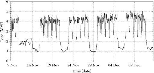
FIGURE 16.2 Examples of x-outliers in a load curve.

16.2.2 METHOD FOR CLEANSING OUTLIERS

The method for cleansing outliers includes the following steps: (1) load curve data are represented using a smoothing curve, which captures the general trend of the data; (2) a confidence interval on the smoothing curve is built to identify localized y-outliers; (3) the smoothing curve is modeled by a sequence of valleys and peaks, called ∪ shapes and ∩ shapes, which are the potential places where x-outliers could occur; (4) x-outliers are identified as the valleys, peaks, or both that do not repeat; and (5) the detected outliers are approximately repaired [8,9,10].

16.2.2.1 Kernel Function Representation of Load Curve

The first step in detecting outliers is to model the intrinsic patterns of load curve data by a smoothing curve. This step can be performed by standard smoothing techniques. Given a time series of load curve data, T = {(t_i;, y_i)} (i = 1, …, n) where y_i is the load value at the time point t_i, the regression relationship of the data can be modeled by a continuous function [10]:

$y_{i} = m (t_{i}) + ε_{i} (i = 1, \dots, n)$ $y_{i} = m (t_{i}) + ε_{i} (i = 1, \dots, n)$

(16.1)

This function is composed of the regression function m and the observation error ε_i. The estimated load value in the regression function at time t is modeled in a form of nonparametric regression by

$\overset{⌢}{m} (t) = \frac{1}{n} \sum_{i = 1}^{n} w_{i} (t) y_{i}$ $\overset{⌢}{m} (t) = \frac{1}{n} \sum_{i = 1}^{n} w_{i} (t) y_{i}$

(16.2)

where w_i(t) (i= 1,⋯,n) denotes a sequence of weights. Equation 16.2 is called the smoothing curve, in which w_i(t) is the weight of the point (t_i, y_i) at time t in the estimation of the smoothing value. The estimation is neighborhood based in the sense that the further t_i is from t, the less weight is given to the point (t_i, y_i). In the kernel smoothing, w_i(t) is given by

$w_{i} (t) = \frac{K e r n_{h} (t - t_{i})}{{\overset{⌢}{f}}_{h} (t)}$ $w_{i} (t) = \frac{K e r n_{h} (t - t_{i})}{{\overset{⌢}{f}}_{h} (t)}$

(16.3)

where

$K e r n_{h} (t) = \frac{1}{h} K e r n (\frac{t}{h})$ $K e r n_{h} (t) = \frac{1}{h} K e r n (\frac{t}{h})$

(16.4)

is the kernel with the scale factor h. By using the Rosenblatt–Parzen kernel density estimator [11] of the density of t

${\overset{⌢}{f}}_{h} (t) = n^{- 1} \sum_{i = 1}^{n} K e r n_{h} (t - t_{i})$ ${\overset{⌢}{f}}_{h} (t) = n^{- 1} \sum_{i = 1}^{n} K e r n_{h} (t - t_{i})$

(16.5)

the Nadaraya–Watson estimator [11] for Equation 16.2 is obtained as follows:

$\overset{⌢}{m} (t) = \frac{\sum_{i = 1}^{n} K e r n_{h} (t - t_{i}) y i}{\sum_{i = 1}^{n} K e r n_{h} (t - t_{i})}$ $\overset{⌢}{m} (t) = \frac{\sum_{i = 1}^{n} K e r n_{h} (t - t_{i}) y i}{\sum_{i = 1}^{n} K e r n_{h} (t - t_{i})}$

(16.6)

The shape of the kernel weights is determined by the function Kern, whereas the size of weights is parameterized by h, which is called bandwidth and referred to below as smoothing parameter. A larger h corresponds to a smoother curve. The kernel function Kern can be chosen to be the normal probability density function [11], that is,

$K e r n (t) = \frac{1}{\sqrt{2 π}} e^{- (1 / 2) t^{2}}$ $K e r n (t) = \frac{1}{\sqrt{2 π}} e^{- (1 / 2) t^{2}}$

(16.7)

16.2.2.2 Confidence Interval for Identifying y-Outliers

With a smoothing curve expressed by kernel functions, a localized y-axis outlier can be easily identified by building a confidence interval for normal load data on the smoothing curve. An observation within the confidence interval is considered normal and an observation outside the confidence interval is considered invalid data. The error term ε_i in Equation 16.1 is assumed to be normally and independently distributed with the mean of zero and constant variance σ². Under this assumption, the confidence interval of a load data point can be computed by its estimated value plus or minus a multiple of the error. The estimated error s_i(est) is given by [12]

$s_{i} (est) = \sqrt{MSE+ s_{i}^{2} ({\hat{y}}_{i})}$ $s_{i} (est) = \sqrt{MSE+ s_{i}^{2} ({\hat{y}}_{i})}$

(16.8)

where MSE is the error mean square:

$MSE = \frac{1}{n - d} {\sum_{i = 1}^{n} (y_{i} - {\hat{y}}_{i})}^{2}$ $MSE = \frac{1}{n - d} {\sum_{i = 1}^{n} (y_{i} - {\hat{y}}_{i})}^{2}$

(16.9)

and is the sampling variance of load at time point t_i and is given by $s_{i}^{2} ({\hat{y}}_{i})$ $s_{i}^{2} ({\hat{y}}_{i})$

$s_{i}^{2} ({\hat{y}}_{i}) = {WW}^{T} \times MSE$ $s_{i}^{2} ({\hat{y}}_{i}) = {WW}^{T} \times MSE$

(16.10)

where W is called the hat matrix and is calculated by [13]

$W = \frac{1}{n} [\begin{matrix} W_{1} (t_{1}) & W_{2} (t_{1}) & \dots & W_{n} (t_{1}) \\ W_{1} (t_{2}) & W_{2} (t_{2}) & \dots & W_{n} (t_{2}) \\ ⋮ & ⋮ & \dots & ⋮ \\ W_{1} (t_{n}) & W_{2} (t_{n}) & \dots & W_{n} (t_{n}) \end{matrix}]$ $W = \frac{1}{n} [\begin{matrix} W_{1} (t_{1}) & W_{2} (t_{1}) & \dots & W_{n} (t_{1}) \\ W_{1} (t_{2}) & W_{2} (t_{2}) & \dots & W_{n} (t_{2}) \\ ⋮ & ⋮ & \dots & ⋮ \\ W_{1} (t_{n}) & W_{2} (t_{n}) & \dots & W_{n} (t_{n}) \end{matrix}]$

(16.11)

where W_i(t_j) corresponds to the weight of observation at time t_i for estimating the load value at time t_j Note that d in Equation 16.9 is the number of degrees of freedom of the fitted load curve data and can be computed by the trace of the hat matrix W.

For a given significance level α, the confidence interval at time t_i is estimated by

$[{\hat{y}}_{i} - z_{1 - α / 2} \times s_{i} (est), {\hat{y}}_{i} + z_{1 - α / 2} \times s_{i} (est)]$ $[{\hat{y}}_{i} - z_{1 - α / 2} \times s_{i} (est), {\hat{y}}_{i} + z_{1 - α / 2} \times s_{i} (est)]$

(16.12)

where z_1−α/2 is the 100(1 – α/2) percentile of the standard normal distribution. For example, if the 0.05 significance level (α=0.05) is chosen, the corresponding z_1−α/2is 1.96. This means that a normal observation would fall in the confidence interval given by Equation 16.12 with a probability of 95%, or, equivalently, that the probability that a data point located outside the interval is invalid is 95%.

16.2.2.3 Candidates for x-Outliers

An x outlier has an unusual trend against the periodicity. With the trend of the load curve being modeled by the smoothing curve, an x outlier tends to occur at a “valley” or a “peak” of the smoothing curve, where the smoothing curve has local minimal or maximal values. To formally define the location of such valleys and peaks, we first introduce some terminologies.

The slope at time t_i for a smoothing curve ${(t_{i}, {\hat{m}}_{i})}_{i = 1}^{n}$ ${(t_{i}, {\hat{m}}_{i})}_{i = 1}^{n}$ is defined by △m_i/△t_i, where $Δ m_{i} = {\hat{m}}_{i} - {\hat{m}}_{i - 1}$ $Δ m_{i} = {\hat{m}}_{i} - {\hat{m}}_{i - 1}$ , △t_i = t_i—t_i-1, for 2≤i≤n. A time t in an interval is called a steep time point if the absolute value of the slope at time t is the maximum in the interval. In other words, at a steep time point, the load increases or decreases at the maximum rate in the interval. Note that there could be more than one steep time point in an interval. An interval [a, b] is maximal-decreasing if the slope at every time point in [a, b] is ≤0 and any interval containing [a, b] has at least one point with a positive slope. For two time points c and c′; in a maximal-decreasing interval [a, b], [c, b] is convex-decreasing if c is the rightmost steep time point in [a, b], and [a, c′] is concave-decreasing if c′ is the leftmost steep time point in [a, b]. In Figure 16.3, the numbers on the smoothing curve are the slopes of the smoothing curve, and the horizontal axis is time; [t₁, t₅] is a maximal-decreasing interval; and t₃ and t₄ are two steep time points in [t₁, t₅]. Since t₄ is the rightmost steep time point in [t₁, t₅], [t₄, t₅] is a convex-decreasing interval, but [t₃, t₅] is not, while [t₁, t₃] is a concave-decreasing interval.

Similarly, we can define maximal-increasing intervals, concave-increasing intervals, and convex-increasing intervals. In Figure 16.3, [t₆, t₁₀] is a maximal-increasing interval, t₈ and t₉ are steep time points, [t₆, t₈] is a convex-increasing interval because t₈ is the leftmost steep time point in [t₆, t₁₀], and [t₉, t₁₀] is a concave-increasing interval.

The following definitions formalize the notions of valleys and peaks.

Definition of ∪ shape: For a smoothing curve, a ∪ shape is a subcurve $T_{\cup} = {(t_{p}, {\hat{m}}_{p})}_{p = i}^{j}$ $T_{\cup} = {(t_{p}, {\hat{m}}_{p})}_{p = i}^{j}$ such that, for some k with i≤k≤j,[i, k] is a convex-decreasing interval and [k + 1, j] is a convex-increasing interval.

Definition of ∩ shape: For a smoothing curve, a ∩ shape is a subcurve $T_{\cap} = {(t_{p}, {\hat{m}}_{p})}_{p = i}^{j}$ $T_{\cap} = {(t_{p}, {\hat{m}}_{p})}_{p = i}^{j}$ such that, for some k with i≤k≤j, [i, k] is a concave-increasing interval and [k + 1, j] is a concave-decreasing interval.

In Figure 16.3, the curve [t₄, t₈] is a ∪ shape formed by a convex-decreasing interval [t₄, t₅] and a convex-increasing interval [t₆, t₈]. The curve [t₉, t₁₂] is a ∩ shape formed by a concave-increasing interval [t₉, t₁₀] and a concave-decreasing interval [t₁₁, t₁₂]. Notice that the adjacent ∪ shape and ∩ shape overlap at one point at most. Let us see the adjacent ∪ shape [t₄, t₈] and ∩ shape [t₉, t₁₂] in Figure 16.3. The ∪ shape [t₄, t₈] must end at the leftmost steep time point t₈ and the ∩ shape [t₉, t₁₂] must start at the rightmost steep time point t₉. Intuitively, ∪ shapes and ∩ shapes capture the regions on the smoothing curve where the raw load curve has large drops and large rises. Such regions are the potential places where x-outliers may occur. Therefore, ∪ shapes and ∩ shapes are candidate regions for outliers. All candidate regions can be found by computing ∪ shapes and ∩ shapes following their definitions.

FIGURE 16.3 Explanation of the terminologies in smoothing curve [t₁, t₁₂].

16.2.2.4 Identifying x-Outliers

Candidate regions with ∪ shapes and ∩ shapes are extracted based on local neighborhood information (i.e., valleys and peaks). Whether a candidate region contains a real outlier depends on whether the data in the region deviates from the periodicity. A candidate is not a real outlier if similar load data occur regularly in other periods according to the periodicity. The similarity should take into account background noise and time shifting of periodicity.

To identify all outliers, we consider every candidate region r found in the previous step. Let C* denote the portion of the raw load curve data contained in r. We want to emphasize that C* contains raw data in the load curve, not the data in the smoothing curve. If the data in C* occur approximately in the corresponding regions in different periods, C* is not a real outlier but a part of the periodicity. To differentiate this, we extract all the subload curves C₁, C₂, ⋯, C_k, where each C_i is the portion of the raw load curve in the corresponding region of C* in the ith period. If C* is “similar” to the majority of C₁, C₂, ⋯, C_k, C* is considered normal; otherwise, C* is considered a real outlier.

The remaining question is how to measure the similarity between two subcurves C* and C_i with the same length. There are two considerations in choosing the similarity measure. First, the similarity measure should be less sensitive to background noise. For example, the two load curves in Figure 16.4 should be considered similar despite some variability at the first peak due to background noise. Second, the similarity measure should be less sensitive to time shifting and stretching commonly observed in load curve data. For example, load curves T_A and T_B in Figure 16.5 should be considered similar despite minor time shifting and stretching.

The Euclidean distance that is commonly used is not suitable for our purpose because it is sensitive to time shifting and stretching. If the Euclidean distance were used, the two curves T_A and T_B in Figure 16.5 would be recognized as dissimilar. The dynamic time warping distance for two sequences [14] is not suitable either, since it would pair up all points of two sequences in comparison, making it impossible to skip noisy points.

What we need is a similarity measure that will examine a small neighborhood in search of matching points and skip noisy points. For this purpose, the longest common subsequence (LCSS) [15] concept can be adopted. LCSS is a coarse-grained similarity measure in the sense that it measures similarity in terms of “trends” instead of exact points. Below, we describe how LCSS is extended to measure the similarity of load curves.

FIGURE 16.4 Two similar load curves with noise.

FIGURE 16.5 Two similar load curves with time shifting and stretching.

Given two subload curves A = 〈a₁, a₂, ⋯, a_m〉 and B = 〈b₁, b₂, b_n), which correspond to C* and C_i, we want to find the LCSS common to both A and B. The idea is as follows. To allow time shifting and stretching, a_i and b_j that are within some time proximity are examined for matching. If these load points are similar, they are considered as a match and are kept. Dissimilar values in one or both load curves are dropped. Mathematically, given an integer δ and a real value ε, the cumulative similarity S_i,j(A,B) or S_i,j is defined as follows:

$S_{i, j} = {\begin{matrix} 0, & if i = 0 \lor j = 0 \\ 1 + S_{i - 1, j - 1} & if | a_{i} - b_{j} | \leq ε \land | i - j | \leq δ \\ \max (S_{i, j - 1}, S_{i - 1, j}) & otherwise \end{matrix}$ $S_{i, j} = {\begin{matrix} 0, & if i = 0 \lor j = 0 \\ 1 + S_{i - 1, j - 1} & if | a_{i} - b_{j} | \leq ε \land | i - j | \leq δ \\ \max (S_{i, j - 1}, S_{i - 1, j}) & otherwise \end{matrix}$

(16.13)

In Equation 16.13, the first if statement does the initialization for the shortest prefix. The second if statement builds the similarity recursively: if |a_i – b_j|≤ ε and if a_i and b_j are close enough in time, that is, |i –j|≤ δ, a_i and b_j are matched and the similarity is incremented. Note that ε represents a tolerance of noise in load value and δ represents a tolerance of time shifting and stretching.

Let |A| and |B| be the length of A and B, respectively. The LCSS similarity of A and B is given by

$γ (δ, ε, A, B) = \frac{S | A | \cdot | B |}{\min (| A |, | B |)}$ $γ (δ, ε, A, B) = \frac{S | A | \cdot | B |}{\min (| A |, | B |)}$

(16.14)

where S_|A|.|B| is the length of the common subsequence to both A and B, which is cumulatively computed by Equation 16.13. For a user-specified threshold θ, we say that A and B are similar if

$γ (δ, ε, A, B) \geq θ$ $γ (δ, ε, A, B) \geq θ$

(16.15)

16.2.3 REPAIRING OUTLIERS

Detected outliers should be repaired before the load curve can be used for calculating BLCFs or other applications. Suppose that we want to repair an outlier C*. Some valid data must be selected to replace the load data of C*. The replacement data can be derived from the normal data in the corresponding time interval in other periods with an adjustment for the increasing or decreasing long-term trends over time. This is expressed as the following multiplicative model [16]:

$Y (t_{i}) = T (t_{i}) \times (t_{i})$ $Y (t_{i}) = T (t_{i}) \times (t_{i})$

(16.16)

where Y(t_i) represents the value that will replace the abnormal value at a time t_i belonging to an outlier, T(t_i) represents the load value in the long-term trend, and R(t_i) represents the periodic index, that is, how much the load curve deviates from the long-term trend at time t_i.

It is possible to estimate T(t_i) by the smoothing curve defined in Equation 16.2 with an appropriate smoothness level (bandwidth). However, in the presence of outliers, the smoothing curve may contain invalid data around the outliers to be replaced. To address this problem, all outliers in the load curve are replaced, first, by the average of the data at the corresponding time in the previous and following periods. If load points at these times are also outliers themselves, the corresponding data from earlier and later periods will be examined until normal data are obtained. After filling in such average values for all outliers, a new smoothing curve is regenerated using Equation 16.2 and is used to estimate T(t_i).

The periodic index R(t_i) for a time t_i belonging to an outlier is estimated by the average of the periodic indexes at the corresponding time of its previous and following periods, that is,

$R (t_{i}) = \frac{1}{2} (R (t_{i} - l) + R (t_{i} + l))$ $R (t_{i}) = \frac{1}{2} (R (t_{i} - l) + R (t_{i} + l))$

(16.17)

where l is the length of the periodicity. If the data at the previous and next periods are outliers, earlier and later periods are examined until normal data are obtained. Note that, for a time t_i not belonging to an outlier, the periodic index at t_i is computed by its definition:

$R (t_{i}) = \frac{y_{i}}{T (t_{i})}$ $R (t_{i}) = \frac{y_{i}}{T (t_{i})}$

(16.18)

where y_i is the load at time t_i. After T(t_i) and R(t_i) for an outlier are obtained, Equation 16.16 is used to produce the replacement value Y(t_i).

16.2.4 SELECTION OF PARAMETERS

The method described above uses several parameters: the smoothing parameter h (see Equation 16.4), the load stretching threshold ε and the time stretching threshold δ (see Equation 16.13), and the LCSS similarity threshold θ (see Equation 16.15). How should the values of these parameters be set? One approach is to use some statistically “optimal” setting, such as the optimal smoothing parameter [17]. In applications where the user has background knowledge, the user often desires to have control over a small number of settings. A practical approach is to provide a mechanism that helps the user to identify a proper setting of parameters in such a case. We use the smoothing parameter h as an example below, and a similar approach can be applied to other parameters.

FIGURE 16.6 An actual load curve, the smoothing curve, and identified x-outliers.

A larger h produces a smoother smoothing curve, and thus models the load data in less detail. In practice, we do not have to make a choice in advance. A software tool with a user-friendly interface has been developed, which allows the user to slide a bar for the smoothing parameter and displays the smoothing curve and the identified outliers to the user interactively. Based on visual inspection of the raw data, smoothing curve, and identified outliers, the user can either accept the results or slide the bar again for a different choice of h and get a display of the new smoothing curve and outliers based on the new choice of h. This is analogous to sliding the bar at the lower right of the Word window for setting the font size of a document. With such sliding bars, a user often quickly converges to what he or she considers to be the best setting.

As an experiment, the method was applied to an actual industrial load curve in the system of BC Hydro, Canada. This load curve includes hourly MW loads for the 6 years from October 2004 to October 2010, with 24 ⨯ 365 ⨯ 6 = 52,560 observed records. Figure 16.6 shows the raw load records, the smoothing curve (by the bold line) obtained using a specific smoothing parameter h [8], and the x-outliers (marked by each rectangle) detected by the proposed method. It can be seen that the smoothing curve models the load curve properly and there is no false-positive or false-negative error in detecting the x-outliers.

16.3 BUS LOAD COINCIDENCE FACTORS

Once outliers in historical load curves are cleansed, calculating BLCFs using load curve data is straightforward. This section illustrates the basic concept and procedure of calculating BLCF, and Section 16.4 will present an example to demonstrate the application of BLCF to power system analysis.

16.3.1 BASIC CONCEPT OF BLCF

Once load curves at all considered buses are cleansed, it is straightforward to calculate the BLCFs. The BLCF is an important concept in power system analyses, particularly in power flow studies [4]. The load forecast generally provides annual peak values for the whole system, each region, and individual substations. As mentioned in Section 16.1, loads at substations never reach their peaks at the same point in time. To perform a power flow study at the annual system or regional peak, or at a percentage level of the annual peak, which may be a seasonal peak or valley, we must calculate bus loads corresponding to the peak or the level of the peak. The BLCFs at the buses are used for this purpose.

The concept of BLCF is illustrated using Figure 16.7. For simplicity, only two substation load curves are considered. The total load curve, which is the sum of the two substation load curves, can be viewed as the system (or regional) load curve. Points A, E, and D are the peaks of the system and two substation load curves, respectively. Apparently, they do not occur at the same time. Points C and B represent the load points of the two substations corresponding to the system (or regional) peak. The BLCFs of the two substations are defined as

${BLCF}_{1} = \frac{L_{C}}{L_{E}}$ ${BLCF}_{1} = \frac{L_{C}}{L_{E}}$

(16.19)

${BLCF}_{2} = \frac{L_{B}}{L_{D}}$ ${BLCF}_{2} = \frac{L_{B}}{L_{D}}$

(16.20)

where L_C and L_E are the loads at Points C and E in the load curve 1 for Substation 1, and L_B and L_D are the loads at Points B and D in the load curve 2 for Substation 2.

FIGURE 16.7 Concept of BLCF.

Obviously, cleansed load curve data are important to accurately calculate BLCF. For instance, if the load around Point B, C, D, or E is corrupted, we will get a distorted BLCF value. Even if the load at Point B or C is valid data, a reduced L_D or L_E will overestimate the BLCF value and an elevated L_D or L_E will underestimate the BLCF value.

Using the example shown in Figure 16.7, we defined the BLCF corresponding to the system peak. For a given load point in a system or regional load curve, the corresponding time point on the x-axis is called the reference point. In this sense, BLCFs can be calculated for any different reference points on a system or regional load curve (such as the annual peak, winter or summer peak, winter or summer valley). BLCFs can be also calculated for different load categories (such as industrial, residential, or commercial customers or their combinations) using a similar concept. Apparently, BLCFs vary dynamically from year to year, as the load curve data change every year. BLCFs should be estimated using multiple years of load data and updated each year. There are uncertainties around load data points. The system or regional peak is different in value and moves around in different years, and various periodicities in a load curve may be shifted. To tackle the uncertainties, instead of using the load value at each single point (such as A, B, C, D, or E), the average of a certain number of loads around each point should be used.

Once the BLCFs are estimated, the bus loads corresponding to any reference point on a system or regional load curve can be calculated using the BLCF values for that reference point and the forecasted peaks of substation loads.

16.3.2 PROCEDURE FOR CALCULATING BLCF

In the procedure described below, the annual system peak in a 1-year period is used as a reference point to indicate how to estimate the BLCF values and calculate bus loads corresponding to the reference point. The procedure for estimating the BLCFs corresponding to other reference points (a percentage level of the annual system peak or the maximum/minimum load value in a specified period, such as winter or summer) in a system or region is similar.

The procedure includes the following steps [18]:

1. The invalid data for yearly load curves at all considered substations are cleansed using the method given in Section 16.2, including identification and repairing of invalid data.

2. All the yearly substation load curves are summed up to obtain the yearly system load curve. The maximum hourly load value (peak) in the yearly system load curve is determined and is assumed to be X MW. The corresponding time point on the x-axis is called the reference point.

3. N hourly load points on the system load curve that are closest to the X MW in the load values are determined, where N (such as 24 or 48) is a proper number for handling the uncertainty of the system peak. In the case where the annual system peak is selected as the reference point, the N hourly load values include the system peak, itself being X MW, with others being smaller than or equal to X MW. In other cases in which a nonannual system peak is selected as the reference point, some of the N selected hourly load values may be larger than X MW but others may be smaller than X MW.

4. M annual largest hourly load values on the yearly load curve of each individual substation are determined, where M is a proper number for handling the uncertainty of the substation load peak and may or may not be equal to N, depending on a judgment on the degree of uncertainty of the substation load peak. Let L_ki(P) denote the MW load at the kth point of the M hourly load points in the ith substation load curve.

5. We locate the N points on each yearly substation load curve that correspond to the same time points as the N load points on the yearly system load curve, which have been determined in Step 3. Let L_ji denote the MW load at the jth point of the N selected hourly load points in the ith substation load curve. The BLCF corresponding to the selected reference point for the ith substation is estimated by

${BLCF}_{i} = \frac{1}{N} \sum_{j = 1}^{N} \frac{L_{j i}}{[\sum_{k = 1}^{k = M} L_{k i} (P)] / M}$ ${BLCF}_{i} = \frac{1}{N} \sum_{j = 1}^{N} \frac{L_{j i}}{[\sum_{k = 1}^{k = M} L_{k i} (P)] / M}$

(16.21)

6. There are always some differences in the yearly load curves of a substation in different years. In many cases, the differences may be relatively small, as load customers supplied by the substation usually maintain their electricity consumption behaviors. In other cases, the differences may be relatively large because the electricity consumption behaviors of some customers change over the years. To deal with the possible changes, it is better to repeat Steps 1–5 for more than 1 year’s load curve data. On the other hand, we should not use too many years’ data, since cumulative changes may be so significant that data from previous years are no longer representative of the most recent pattern. We suggest considering a time frame of the past 3 years for obtaining three BLCF values for each substation. There are three possibilities, as follows:

a. Only 1 year’s load curve data are available. In this case, the BLCF for this year is used.

b. Two years’ load curve data are available. In this case, the difference between the two BLCF values is calculated as a percentage with respect to the larger value.

i.	If the difference is smaller than or equal to a threshold (such as 5%–10%), the average of the two BLCF values is used as the final BLCF.
ii.	If the difference is larger than the threshold, the BLCF from the most recent year’s load curve is used as the final BLCF.

c. Three years’ load curve data are available. In this case, the differences between each pair of the three BLCF values are calculated as a percentage with respect to the largest value.

i.	If all the three differences are smaller than the threshold, the average of the three BLCF values is used as the final BLCF.
ii.	If two of the three differences are smaller than the threshold, the average of the larger two BLCF values is used as the final BLCF.
iii.	If only one of the three differences is smaller than the threshold, the average of the two BLCF values corresponding to this difference is used as the final BLCF.
iv.	If all the three differences are larger than the threshold, the BLCF from the most recent year’s load curve is used as the final BLCF.

7. The MW load of each substation corresponding to the selected reference point (such as the annual system peak, or a percentage level of the annual system peak, or the maximum or minimum load value in a selected period) can be calculated using the BLCF value of each substation and the forecast peak load for each substation in the considered year, by

$L_{i} (MW) = L_{i} (F) \times {BLCF}_{i}$ $L_{i} (MW) = L_{i} (F) \times {BLCF}_{i}$

(16.22)

where L_i(MW) is the MW load at the ith substation (bus) corresponding to the reference point and L_i(F) is the forecasted peak load for the ith substation.

It should be pointed out that the word “system” in the above description can refer to a whole system, a region or area, a subregion or subarea, or a substation group.

16.4 APPLICATION OF BLCF TO SYSTEM ANALYSIS

A real-life case is used in this section to demonstrate the application of BLCF to system analysis.

16.4.1 STUDIED SYSTEM AND LOAD CURVE DATA

Figure 16.8 shows a transmission network supplying power to a subarea of BC Hydro in Canada. The subarea includes three substations named YVR, SEA, and RIM. The power is supplied from the upstream substation KI2 through two 60 kV transmission circuits named 60L43 and 60L44. Each circuit includes three sections marked by A, B, and C. Sections A and B are overhead lines and Section C is an underground cable. The MVA ratings of the three sections of each circuit in winter and summer are listed in Table 16.1.

The cleansed hourly load curves at the three substations in 2006/2007 are shown in Figure 16.9. By summing up the loads of the three substations at every hour, the total load curve of the subarea is created, as shown in Figure 16.10, where the summer and winter peak periods are framed by the two dashed line rectangles. This subarea has its annual peak in winter, which appears on November 29, at 5:00 pm, for this particular year.

The maximum loading levels on the two circuits (60L43 and 60L44) occur at the same time point as the subarea peak. The power flows at the maximum loading levels on November 29, 2006 at 5:00 p.m. are displayed in Figure 16.11. It can be seen that the actual maximum loading levels in the normal state are as follows:

In the normal state, 60L44 loading = 48.2/156 = 30.9%

In N-1 contingency states, the maximum loading level can be calculated by contingency analysis. It is 105.9/156 = 67.9%.

FIGURE 16.8 The subarea power supply network.

TABLE 16.1
Rating of the Two Circuits

	Winter Rating	Summer Rating
Circuit Section	(MVA) (10°c)	(MVA) (30°c)
60L43A and 60L44A	156	121
60L43B and 60L44B	100	78
60L43C and 60L44C	68.5	63

16.4.2 BUS LOAD COINCIDENCE FACTORS AT THE THREE SUBSTATIONS

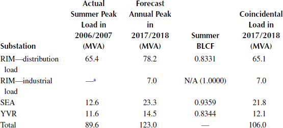
The BLCFs are calculated using the method in Section 16.3 and the historical load curve data at the three substations. The BLCF values obtained using the subarea winter peak (which is the annual peak in this example) and summer peak as the reference points are given in Tables 16.2 and 16.3, together with the forecast annual (winter) peak loads in 2017/2018 and the calculated coincidence bus loads in 2017/2018. It is important to appreciate that a coincident load for the subarea summer peak as a reference point should be, and is still, calculated using the forecasted annual peak (i.e., the winter peak in this case) multiplied by its summer BLCF, since a BLCF is always defined as a load at the reference point divided by its annual peak. To make a comparison, the winter and summer peak loads of the three substations in 2006/2007 are also given in the two tables. Note that the load at the RIM substation includes two components: distribution and industrial customers. The industrial customer at RIM will not be in service until 2017/2018, and therefore its historical load curve data are not available for calculating the BLCF. In this case, the BLCF can be assumed to be 1.0. Such an assumption creates a relatively high loading level, which can lead to a more secure decision in system operation and planning. A small part of the distribution load at RIM will be transferred to another substation by 2017/2018.

FIGURE 16.9 The cleansed hourly load curves at the three substations.

FIGURE 16.10 The load curve of the subarea.

In the normal state, 60L43 loading = 56.5/156 = 36.2%

FIGURE 16.11 The power flows at the actual annual maximum loading levels in 2006/2007.

It can be observed that the total load in the subarea is increased from 105.8 MW in 2006/2007 to 123 MW in 2017/2018. This is translated into an average annual growth rate of 1.5% (1.56 MW/year). The difference between the forecasted (noncoincidental) total load and the coincidental total load is 123–119=4.0 MW. This is equivalent to the load increase percentage in about 2 years. In other words, if the coincidental loads are used for a planning purpose, this may lead to approximately 2 years’ delay of the system reinforcement required by the load growth in this subarea. This observation can be verified by the power flow studies given in the next subsection.

TABLE 16.2
BLCFs and Coincidence Loads for the Winter Peak at the Three Substations

a —The industrial customer is not yet in service and the load profile is therefore not available.

TABLE 16.3
BLCFs and Coincidence Loads for the Summer Peak at the Three substations

16.4.3 POWER FLOW ANALYSIS USING THE BUS LOAD COINCIDENCE FACTORS

The power flow studies for the subarea network are performed using the noncoincidental and coincidental substation loads in 2017/2018. The following four cases are considered:

Case 1: Noncoincidental winter peak loads, which refer to the forecasted annual peaks at the given three substations.

Case 2: Noncoincidental summer peak loads. For utilities having the annual peak in winter, although load forecast departments at the utilities may also provide the forecasted summer peak for the whole system (or areas) in addition to the forecasted winter peaks for the whole system (areas) and all substations, they generally do not provide the forecasted summer peaks for individual substations. In the existing practice of utilities, a common approach is to calculate substation loads at the system summer peak point by proportionally scaling down from the annual substation peaks using the same ratio of the system (area) winter peak with regard to the system (area) summer peak. In this case, the noncoincidental summer peak loads are obtained using this approach.

Case 3: Coincident winter peak loads. In this case, the substation loads are calculated using their BLCFs corresponding to the winter (annual) subarea peak.

Case 4: Coincident summer peak loads. In this case, the substation loads are calculated using their BLCFs corresponding to the summer subarea peak.

The loading levels in the four cases are summarized in Table 16.4. The power flows for the four cases in the normal states (no component outage) are shown in Figures 16.12 through 16.15, respectively. The following observations can be made:

• o The difference in the maximum loading level for N-1 contingency states between noncoincidental and coincidental winter peak cases is 2.7% (78.7%-76%). This is equivalent to a loading level increase in about 2 years, as the annual average loading level increase is approximately (118.6-105.9)/11/105.9 = 1.1%. In other words, using the coincidental loads in the power flow analysis can delay the upgrade of the two circuits by approximately 2 years. This loading level analysis is consistent with the direct comparison between the forecasted and coincidental total loads, although their percentages are slightly different.

TABLE 16.4
Loading Levels in the Four Cases

FIGURE 16.12 The power flows in Case 1 (using the noncoincidental winter peak loads in 2017/2018).

FIGURE 16.13 The power flows in Case 2 (using the noncoincidental summer peak loads in 2017/2018).

FIGURE 16.14 The power flows in Case 3 (using the coincidental winter peak loads in 2017/2018).

FIGURE 16.15 The power flows in Case 4 (using the coincidental summer peak loads in 2017/2018).

• It is noticed that the difference between noncoincidence and coincidence loads for the winter peak is not significant in this particular example. However, such a difference may be quite large in other system cases.

• It should be emphasized that the noncoincidental summer peak using a traditional load-scaling method could result in an overoptimistic case because the circuit loadings based on the coincidental summer peak case are higher. This observation is opposite to that in the winter peak. As a result, the future system reinforcement in this subarea is driven by summer constraints, and therefore a coincidental summer peak case should be developed and used to capture this concern.

• By comparing the results in Cases 3 and 4, it is observed that the percentage loading level in the summer peak is higher than that in the winter peak in this subarea. This implies that the subarea is mainly constrained by the summer rating. This phenomenon can be intuitively judged from the high BLCFs in the summer peak and the high ratio of the summer peak to the winter peak (106/119 = 89.1%) (see Tables 16.2 and 16.3).

16.5 CONCLUSIONS

Load curve data at substations play an important role in data analytics of smart grids. Implementation of smart meters makes it possible to record time-varying loads at end users or on feeders at intervals of seconds or minutes and to acquire chronological load curve data at all substations. Unfortunately, invalid load data cannot be avoided in the data collection and transfer process, even for smart meters. Therefore, load curve data cleansing is an essential task. This chapter presents a method for load curve data cleansing based on techniques used in data mining and statistics. The method not only effectively identifies both y-outliers and x-outliers but it also repairs the outliers.

Cleansed load curve data are extremely useful information for system analyses and visualization in day-to-day operations and long-term planning. One straightforward application is the calculation of BLCFs at substations. The BLCFs produce an accurate coincidental bus load model in power flow studies. The use of noncoincidental loads in the system analysis may lead to overestimation or underestimation of loading levels in a transmission system and in turn result in overinvestment or system insecurity risk. This chapter proposes an approach and a procedure for estimating BLCFs in power grids. An actual utility subarea system is used to demonstrate the application and benefits of using BLCFs.

* This work is partly supported by a collaborative research and development grant from the Natural Sciences and Engineering Research Council of Canada.

REFERENCES

1. IEEE Standard 399-1990, IEEE Recommended Practice for Power Systems Analysis, IEEE Press, New York, 1990.

2. L. L. Grigsby (editor-in-chief), The Electric Power Engineering Handbook, CRC Press and IEEE Press, Boca Raton, FL, 2001.

3. W. Li, Risk Assessment of Power Systems: Models, Methods, and Applications, IEEE Press and Wiley, New York, 2005.

4. W. Li, Probabilistic Transmission System Planning, IEEE Press and Wiley, Hoboken, NJ, 2011.

5. E. Keogh, J. Lin, S. H. Lee, and H. V. Herle, Finding the most unusual time series subsequence: Algorithms and applications, Knowledge and Information Systems, 11(1), 1–27, 2006.

6. V. J. Hodge and J. Austin, A survey of outlier detection methodologies, Artificial Intelligence Review, 22(2), 5–126, 2004.

7. V. Barnett and T. Lewis, Outliers in Statistical Data, 3rd edn., Wiley, Chichester, 1994.

8. J. Chen, W. Li, A. Lau, J. Cao, and K. Wang, Automated load curve data cleansing in power systems, IEEE PES Transactions on Smart Grid, 1(2), 213–221, 2010.

9. Z. Guo, W. Li, A. Lau, T. Inga-Rojas, and K. Wang, Detecting X-outliers in load curve data in power systems, IEEE Transactions on Power Systems, 27(2), 875–884, 2012.

10. Z. Guo, W. Li, A. Lau, T. Inga-Roja, and K. Wang, Trend-based periodicity detection for load curve data, in IEEE Power and Energy Society General Meeting, July 21–25, Vancouver, BC, 2013.

11. W. Hardle, Applied Nonparametric Regression, Cambridge University Press, New York, 1990.

12. M. H. Kutner, C. J. Nachtsheim, J. Neter, and W. Li, Applied Linear Statistical Models, 5th edn., McGraw-Hill/Irwin, New York, 2004.

13. J. O. Ramsay and B. W. Silverman, Functional Data Analysis, 2nd edn., Springer, New York, 2005.

14. B. Yi, H. Jagadish, and C. Faloutsos, Efficient retrieval of similar time sequences under time warping, in Proceedings of the 14th International Conference on Data Engineering, (ICDE), pp. 201–208, February 23–27, Orlando, FL, 1998.

15. M. Vlachos, G. Kollios, and D. Gunopulos, Discovering similar multi-dimensional trajectories, in Proceedings of the 18th International Conference on Data Engineering, (ICDE), pp. 673–684, 26 February–1 March, San Jose, CA, 2002.

16. D. M. Bourg, Excel Scientific and Engineering Cookbook, O’Reilly, Sebastopol CA, 2006.

17. W. Hardle, M. Muller, S. Sperlich, and A. Werwatz, Nonparametric and Semi-parametric Models, Springer, Berlin, 2004.

18. W. Li, Architecture design and calculation method of load coincidence factor application, BCTC report, BCTC-SPPA-R012, April 1, 2007.

..................Content has been hidden....................

You can't read the all page of ebook, please click here login for view all page.

Table of Contents for Chapter 16 Load Data Cleansing and Bus Load Coincidence Factors

Create new playlist

Sign In

Sign Up

Table of Contents for
Chapter 16 Load Data Cleansing and Bus Load Coincidence Factors