4

Fuzzy Inference Systems

The previous chapter provides the basic concepts of fuzzy logic. This chapter includes a discussion on fuzzy inference system, which is a kind of input–output mapping that exploits the concepts and principles of fuzzy logic. Such systems are widely used in machine control, popularly known as fuzzy control systems. The advantage of fuzzy inference systems is that here the solution to the problem can be cast in terms of familiar human operators. Hence, the human experience can be used in the design of the controller. Engineers developed a variety of fuzzy controllers for both industrial and consumer applications. These include vacuum cleaners, autofocusing camera, air conditioner, low-power refrigerators, dish washer etc. Fuzzy inference systems have been successfully applied to various areas including automatic control, computer vision, expert systems, decision analysis, data classification, and so on. Moreover, these systems are associated with such diverse entities as rule based systems, expert systems, modeling, associative memory etc. These versatile application areas show the multidisciplinary nature of fuzzy inference systems.

4.1  INTRODUCTION

A fuzzy inference system (FIS) is a system that transforms a given input to an output with the help of fuzzy logic. The input-output mapping provided by the fuzzy inference system creates a basis for decision-making process. The procedure followed by a fuzzy inference system is known as fuzzy inference mechanism, or simply fuzzy inference. It makes use of various aspects of fuzzy logic, viz., membership function, fuzzy logical operation, fuzzy IF-THEN rules etc. There are various kinds of fuzzy inference systems. In this chapter we describe the principles of fuzzy inference systems proposed by Ebrahim Mamdani in 1975. It is the most common fuzzy inference methodology and moreover, it is employed in the earliest control system built using fuzzy logic. The fundamental concepts of a fuzzy inference system are explained subsequently along with illustrative examples.

Let us consider a person trying to cross a road while a car is approaching towards him. At what pace should he proceed? It depends on the distance of the approaching car from the person, and its speed. If the car is far away and is running slowly then the person can walk across the road quite leisurely. If the car is far away but approaching fast then he should not try to cross the road leisurely, but a bit faster, say, unhurriedly. However, in case the car is nearby, or is running fast, then he has to cross the road quickly. All these constitute the rule base that guides the pace of the person’s movement across the road.

The sequence of steps followed by a fuzzy inference system for the problem stated above is shown in Fig. 4.1. It presents the basic structure of any fuzzy inference system. The entire fuzzy inference process comprises five steps

1. Fuzzification of the input variables
2. Application of fuzzy operators on the antecedent parts of the rules
3. Evaluation of the fuzzy rules
4. Aggregation of fuzzy sets across the rules
5. Defuzzification of the resultant fuzzy set

The following sections explain these steps briefly.

4.2.  FUZZIFICATION OF THE INPUT VARIABLES

The inputs to a fuzzy inference system are a number of crisp values corresponding to some parameters. For each input, we have to determine the degree to which it belongs to the appropriate fuzzy set through membership function. This is known as fuzzification, the first step of the entire fuzzy inference process.

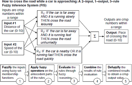
Fig. 4.1. Structure of a fuzzy inference system.

In the present example there are two inputs, the distance of the car from the man, and its speed, both scaled to the range 0–10. There are three rules, and each of them requires that the inputs should be resolved into certain fuzzy linguistic sets. The concerned linguistic values related to the antecedent parts here are, far away (‘the car is far away’), nearby (‘the car is nearby’), running slowly (‘it is running slowly’), and running fast (‘it is running fast’).

Fig. 4.2 shows fuzzification of the car’s distance with respect to the fuzzy set far away. Assuming the distance to be 7 (in the range 0–10) the fuzzy membership is seen to be 0.5 here. The third row in Fig. 4.6 shows the profile of the fuzzy set nearby where the fuzzy membership for distance = 7 is 0.2. Figs. 4.3, 4.4, and 4.6 depict the fuzzification of the other input variable speed = 3 with respect to the fuzzy sets slowly and fast.

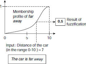
Fig. 4.2. Fuzzification of input variables.

4.3  APPLICATION OF FUZZY OPERATORS ON THE ANTECEDENT PARTS OF THE RULES

The antecedent of a fuzzy rule may consist of a single part or more than one parts joined together with AND, or OR, operators. In this example, each rule has antecedents with two parts. In rules R₁ and R₂ the parts are joined together with the AND operator, and in R₃ they are joined with the OR operator. If, however, we had a rule like ‘IF the car is very close THEN cross the road very quickly’, then, obviously, the antecedent would have been composed of a single part. Fuzzification of inputs determines the degree to which each part of the antecedent (or, just the antecedent, in case it consists of a single part) is satisfied.

When the antecedent of a given rule has more than one parts, we need to apply the appropriate fuzzy operator so that a single number representing the result of the entire antecedent is obtained. The input to the fuzzy operator is two, or more, membership values from the fuzzified input variables and the output is a single truth value. This single truth value is applied to the consequent part of the fuzzy rule to obtain the resultant fuzzy set corresponding to that rule.

 

Table 4.1. Common fuzzy AND, OR methods

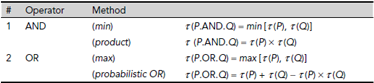
There are various methods of implementing the fuzzy AND and OR operators. The most popular among these, two for each of AND and OR, are summarized in Table 4.1. In the present example the min method of AND, and max method of OR are followed. Fig. 4.3 illustrates the process of applying fuzzy operator on the antecedent part of rule R₁. The first part and the second part of the antecedent produces the membership values 0.5 and 0.6, respectively. The resultant truth value of the entire antecedent is therefore min (0.5, 0.6) = 0.5. A similar process carried out on the rules R₂ and R₃ is shown in Fig. 4.6.

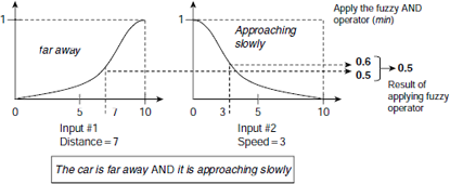
Fig. 4.3. Applying fuzzy operators on the antecedent parts of the rules.

4.4  EVALUATION OF THE FUZZY RULES

Fuzzy rules are evaluated by employing some implication process. The input to the implication process is the number provided by the antecedent and its output is a fuzzy set. This output fuzzy set is obtained by reshaping the fuzzy set corresponding to the consequent part of the rule with the help of the number given by the antecedent.

Fig. 4.4. Evaluation of fuzzy rule during fuzzy inference process.

The implication process is illustrated in Fig. 4.4. The fuzzy set for the consequent of the rule R₁, i.e., cross the road leisurely, has a triangular membership profile as shown in the figure. As a result of applying fuzzy AND operator as the minimum of its operands, the antecedent returns the value 0.5, which is subsequently passed on to the consequent to complete the implication process. The implication process reshapes the membership function of the fuzzy set leisurely by taking the minimum between 0.5, and the membership value of leisurely at any point. The result is a trapezoidal membership function as depicted in the figure. As in the case of fuzzy logic operators there are several implication methods. Among these the min method proposed by Mamdani is followed here. It effectively truncates the fuzzy membership profile of the consequent with the value returned by the antecedent.

It should be noted that the rules of an FIS may have various weights attached to them ranging from 0 to 1. In the present case all rules are assigned the same weight 1. In case a rule has a non-zero but less-than-one weight, it has to be applied on the number given by the antecedent prior to realization of the implication process.

4.5  AGGREGATION OF OUTPUT FUZZY SETS ACROSS THE RULES

Decision-making through a fuzzy inference system has to take into account the contribution of each rule in the system. Therefore the individual fuzzy sets obtained by evaluating the rules must be combined in some manner into a single resultant fuzzy set. This aggregation process takes the truncated membership profiles returned by the implication process as its input, and produces one fuzzy set for each output variable as the output.

Various aggregation methods are used in practice. Taking the maximum among all inputs (max), or taking the algebraic sum of all inputs (sum) are two methods widely employed by the professionals. Fig. 4.5 illustrates the principle of these two methods. In Fig. 4.6, all three rules R₁, R₂, and R₃ are placed together to show how the outputs of all the rules are combined into a single fuzzy set using the max aggregation method.

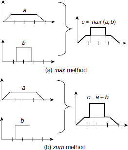
Fig. 4.5. Two popular aggregation methods – max and sum.

4.6  DEFUZZIFICATION OF THE RESULTANT AGGREGATE FUZZY SET

Defuzzification is the process of converting the aggregate output sets into one crisp value for each output variable. This is the last step of a fuzzy inference process. The final desired output for each variable is generally a single number because like the inputs, the outputs too are usually variables signifying physical parameters, e.g., voltage, pressure etc., under control. Since the aggregate of a number of fuzzy sets is itself a fuzzy set and encompass a range of output values, it is not suitable to drive a physical system. It has to be defuzzified in order to resolve into a single output value for the related output variable. There are several defuzzification methods in vogue, viz., centroid method, centre-of-sums (CoS) method, mean-of-maxima (MoM) method etc. These are briefly explained in Fig. 2.6.

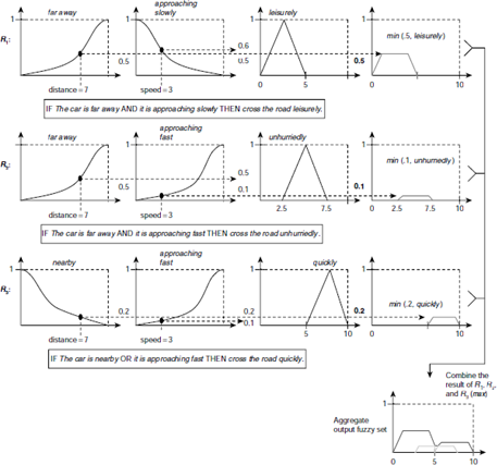
Fig. 4.6. Aggregation of fuzzy sets across the rules.

4.6.1  Centroid Method

The centroid method is also referred to as centre-of-gravity or centre-of-area method. In this method the individual output fuzzy sets are superimposed into a single aggregate fuzzy set (the max method) and then the centroid, or centre-of-gravity, or centre-of-area of the resultant membership profile is taken as the defuzzified output. Fig. 4.7 illustrates the method graphically.

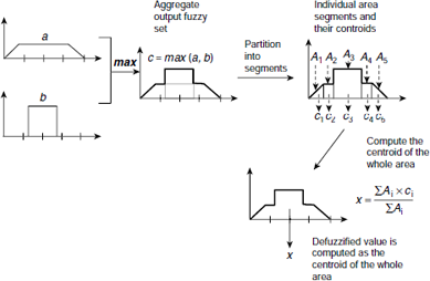
Fig. 4.7. The centroid method of defuzzification.

If the total area under the aggregate output fuzzy set is partitioned into disjoint segments A₁, …, A_k, and the corresponding centroids are c₁, …, c_k, then the centroid of the whole area is obtained as

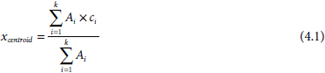
For discrete membership function, the formula is

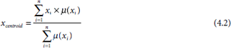
whereas the expression for the centroid in case of continuous membership function is given by

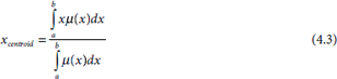
where [a, b] is the domain of x.

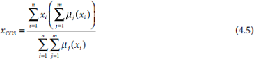
4.6.2  Centre-of-Sums (CoS) Method

The CoS method works almost in the same way as that of the centroid method described earlier. The only difference is, here the aggregate output set is obtained by the sum method rather than the max method. Effectively, this boils down to counting the overlapping areas twice instead of once. Therefore, in CoS method, the areas and the centroids of individual fuzzy sets (obtained as a result of evaluating the fuzzy rules) are computed, and then the defuzzified value of x is obtained as

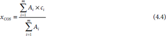
where A₁, ..., A_m, are the areas corresponding to the m number of individual output fuzzy sets and c₁, ..., c_m are respective centroids. The technique of CoS aggregation method is illustrated in Fig. 4.8.

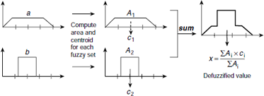
Fig. 4.8. The centre-of-sum (CoS) method of defuzzification

Now consider the situation where the fuzzy sets are discrete. Let the number of sets be m and x₁, ..., x_n be the n number of members. For each member x_i let μ₁(x_i), ..., μ_m(x_i) be the degrees of membership of x_i to the respective fuzzy sets. Then according to the CoS method of defuzzification, the defuzzified value is computed as

4.6.3  Mean-of-Maxima (MoM) Method

MoM is a simple defuzzification method where the highest degree of membership among all fuzzy sets is taken as the output defuzzified value. In case there are more than one elements, say x₁, ..., x_k, having the same highest degree of membership, then the mean of those points is taken as the defuzzified value.

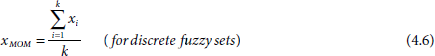
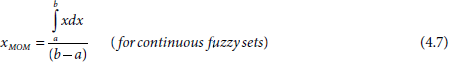
Fig. 4.9 illustrates the MoM method of defuzzification.

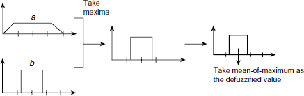
Fig. 4.9. The mean-of-maxima (MoM) method of defuzzification.

In the present example defuzzification is carried out using the CoS method as detailed in Table 4.2. The defuzzified value is computed as

This implies that if the distance of the car is 7 (in the scale of 0–10) and it is approaching with a speed 3 (again in the scale 0–10) then according to the FIS exemplified here the person should cross the road with a pace of 4.25 (in the scale 0–10). The entire fuzzy inference process is schematically depicted in Fig. 4.10.

 

Table 4.2. Computation of areas and centroids

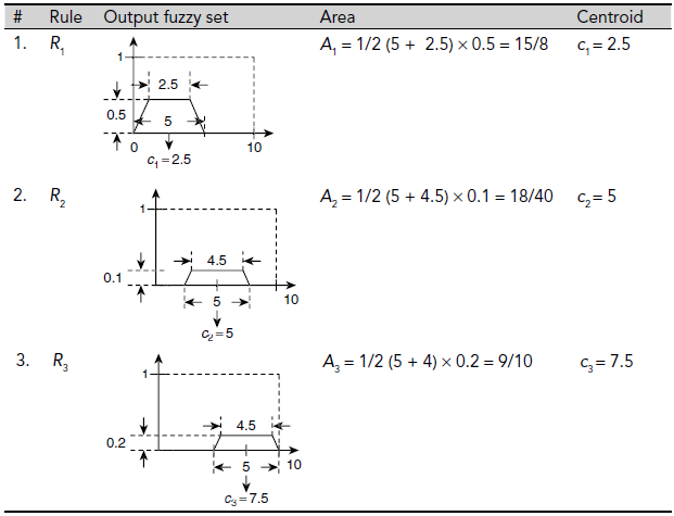
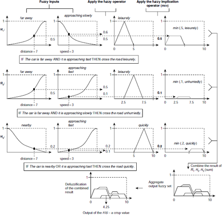
Fig. 4.10. Fuzzy inference process using centre of sums (CoS) method.

4.7  FUZZY CONTROLLERS

Most obvious examples of fuzzy inference systems are the so called fuzzy controllers. These are controlling and decision-making systems that exploit rules involving fuzzy linguistic descriptions for the purpose of controlling a physical process. They employ fuzzy inference process as their functional principle. E. H. Mamdani and S. Assilian have shown in 1974 that a model steam engine could be regulated with the help of a set of fuzzy IF-THEN rules. Since then innumerable fuzzy controllers have been developed for such diverse applications areas as blast furnace, mobile robots, cement kilns, unmanned helicopters, subway trains and so on. As a result of the advent of fuzzy microprocessors, the realm of fuzzy controllers have been extended to consumer electronics and home appliances, e.g., washing machine, vacuum cleaner, camera, air conditioner.

The basic structure of a fuzzy controller is rather simple. It consists of three stages, viz., the input stage, the processing stage, and the output stage (Fig. 4.11).

Fig. 4.11. Basic structure of a fuzzy controller.

Sensor or any other inputs are fed to the controller through the input values and mapped to membership values of appropriate fuzzy sets. This is the fuzzification step. The processing stage utilizes a fuzzy rule base that consists of a number of fuzzy rules. The basic form of a fuzzy rule, as mentioned earlier, is

 

 

where x and y are the input and the output parameters, and A and B are linguistic values. A typical fuzzy rule may look like ‘IF room temperature is cool THEN heater is high’. The ‘IF’ part of a fuzzy rule is known as the ‘antecedent’ and the ‘THEN’ part is called the ‘consequent’. In case of the rule ‘IF room temperature is cool THEN heater is high’ the antecedent is ‘room temperature is cool’ while ‘heater is high’ is the consequent. However, the antecedent of a practical fuzzy rule may consist of several statements of the form ‘x is A’. The general form of a rule in the rule base is

 

The fuzzification step produces the truth values of various statements and depending on these values certain rules of the rule base are fired. The processing stage carries some manipulations on the basis of the fired rules to obtain fuzzy sets relating to the consequent parts of the fired rules. Finally, the outcome of the processing stage on each rule are combined together to arrive at a crisp value for each control parameter. This is carried out during the output stage and is termed as defuzzification. The block diagram shown in Fig. 4.12 gives a bit more detailed picture of a fuzzy controller than provided in Fig. 4.11.

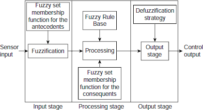
Fig. 4.12. Block diagram of a fuzzy controller.

As discussed earlier in the context of fuzzy inference systems, there are various defuzzification techniques, e.g., centroid, CoS, MoM etc. The designer is to choose the technique most appropriate for his application. In the subsequent parts of this section we present the essential features of two model fuzzy controllers, viz., a fuzzy air-conditioner controller, and a fuzzy cruise controller.

4.7.1  Fuzzy Air Conditioner Controller

Let us consider a highly simplified version of an air-conditioner (AC). Its function is to keep track of the room temperature and regulate the temperature of the air flown into the room. The purpose is to maintain the room temperature at a predefined value. For the sake of simplicity we assume that the AC does not regulate the flow of air into the room, but only the temperature of the air to be flown.

Let T₀ be the desired room temperature. The air conditioner has a thermometer to measure the current room temperature T. The difference ΔT =T – T₀ is the input to the controller. When ΔT > 0, the room is hotter than desired temperature and the AC has to blow cool air into the room so that the room-temperature comes down to T₀. If, on the other hand, ΔT < 0, the room needs to be warmed up and so, the AC is to blow hot air into the room. In order to achieve the required temperature of the air to be blown into the room, a ‘dial’ is turned at the appropriate position within the range [–1, +1]. The scheme is shown in Fig. 4.13.

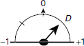
Fig. 4.13. Air-conditioning dial

A positive value of the dial means hot air will be blown, and a negative value means cold air will be blown. The degree of hotness, or coldness, is determined by the magnitude of the dial position. No air is blown when the dial is at 0. The input to the fuzzy controller is ΔT = T – T₀, and the output is D, i.e., the position to which the AC dial is to be turned. Both ΔT and D are crisp values, but the mapping of ΔT to D takes place with the help of fuzzy logic. Various features of the controller are briefly described below.

 

(a) Fuzzy sets: Occasionally, for fuzzy control systems, it is convenient to categorize the strength of the input and the output parameters with the help of certain fuzzy sets referred to as Large Negative (LN), Medium Negative (MN), Small Negative (SN), Zero (ZE), Small Positive (SP), Medium Positive (MP), Large Positive (LP) etc. These are indicative of the magnitude of the respective parameters in the context of the given application. For the system under consideration, the fuzzy sets defined on the input parameter ΔT and D are LN, MN, ZE, MP, and LP. Fig. 4.14 and Fig. 4.15 show the membership profiles of these fuzzy sets. For example, membership of ΔT to Medium Positive (MP) is zero for ΔT ≤ 0, and ΔT ≥ 6. The said membership increases uniformly as ΔT increases from 0 to 3, becomes 1 at 3, and then uniformly diminishes to 0 as ΔT approaches 6 from 3 (Fig. 4.14).

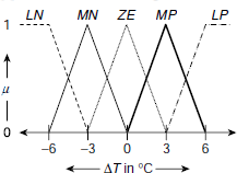
Fig. 4.14. Fuzzy membership functions on ΔT

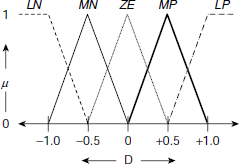
Fig. 4.15. Fuzzy membership functions on D.

All membership functions stated above are of a triangular type, which is widely used in fuzzy controllers. If required, other kinds of membership functions can also be employed.

(b) Fuzzy rule base: The system under consideration has a simple rule base consisting of five fuzzy rules. These are listed below.

 

	R1 :	IF ΔT is LN THEN D is LP.
	R2 :	IF ΔT is MN THEN D is MP.
	R3 :	IF ΔT is ZE THEN D is ZE.
	R4 :	IF ΔT is MP THEN D is MN.
	R5 :	IF ΔT is LP THEN D is LN.

 

The block diagram of the fuzzy inference process for this controller is shown in Fig. 4.16. The input to the system is ΔT, which is first fuzzified with the help of the fuzzy sets membership functions LN, MN, ZE, MP, LP for ΔT. Depending on the result of this fuzzification, some of the rules among R₁, ..., R₅ are fired. As a result of this firing of rules, certain fuzzy sets are obtained out of the specification of LN, MN, ZE, MP, LP for D. These are combined and defuzzified to obtain the crisp value of D as the output.

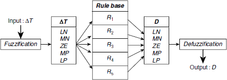
Fig. 4.16. Inference process of the simplified fuzzy air-conditioner controller.

We shall now work out the functionality of the system for the crisp input ΔT = –2.

(a) Fuzzification: Given ΔT = – 2, we compute the degree of membership of ΔT with respect to the fuzzy sets LN, MN, ZE, MP, LP using the respective membership profiles (Fig. 4.17) as follows.

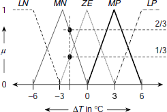
Fig. 4.17. Fuzzy memberships for ΔT = – 2

Since only MN and ZE attain non-zero values, rules R₂, and R₃ are fired. Hence, we have to map these membership values of the antecedents of rules R₂, and R₃ to the corresponding D values in the respective consequents. This is done in the implication phase. Moreover, as the antecedents of all the rules consist of only single parts, the phase of applying fuzzy operators is not relevant here.

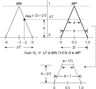
Fig. 4.18. Evaluation of rule R₂

(b) Rule implication: The rule implication process is illustrated in Fig. 4.18 and Fig. 4.19. Fig. 4.18 shows the implication process of Rule R₂ and Fig. 4.19 depicts that for Rule R₃. In case of R₂ the fuzzy membership of input ΔT = – 2 with respect to the fuzzy set MN, i.e., μ_MN (– 2) = 2 / 3, is used to reshape the fuzzy set MP of the consequent part. The result is a fuzzy set with trapezoidal membership function which is shown in the lower region in Fig. 4.18. The area and the centroid (i.e., centre-of-area) this trapezoidal region are computed as area₁ = 4/9, centroid₁ = 0.5. Similarly, area₂ = 5/18, and centroid₂ = 0 are obtained as a result of the implication process carried out on Rule R₂.

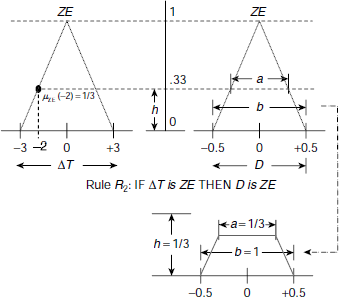
Fig. 4.19. Evaluation of rule R₃

(c) Aggregation and defuzzification: The aggregation and defuzzification process according to the CoS method, centroid method, and MoM method are described below.

(i) Centre-of-sums: Here the defuzzified output is obtained as

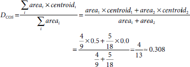
Therefore, when the room temperature is below the set temperature T₀ by 2 degrees (ΔT = –2) the fuzzy AC controller under consideration will set the AC dial at + 0.308 so that air, hot to the extent indicated by the value just mentioned, is blown into the room to bring the room temperature back to T₀.

(ii) Centroid: The first step in this method is to superimpose the outputs of the rule implication process. Accordingly, the trapezoidal regions of Fig. 4.18 and Fig. 4.19 are superimposed to obtain the polygon ABCDEF shown in Fig. 4.20. The polygon ABCDEF is then partitioned into six regions, ΔABJ (A₁), BCIJ (A₂), CKHI (A₃), ΔCDK (A₄), DEGH (A₅), and ΔEFG (A₆). These regions are either rectangles or right-angled triangles. It is easily seen that when the membership functions of the fuzzy sets related to the rules are triangular in shape, the aggregated polygonal region can be partitioned into a numbers of rectangles and right-angled triangles.

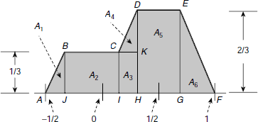
Fig. 4.20. Aggregate region obtained in centroid method of defuzzification.

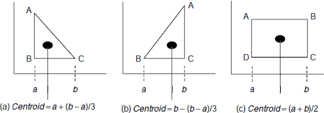
Fig. 4.21. Computing the centroids of rectangular and right-angled triangular regions.

Computation of centroids, i.e., centre-of-areas, of rectangular and right-angled triangular regions is illustrated in Fig. 4.21 (a), (b) and (c). Table 4.3 shows the details of computation of the areas and the centroids of various segments of Fig. 4.20. The crisp output of the fuzzy controller obtained through the centroid method is

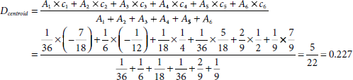
Table 4.3. Computation of areas and centroids of various regions

Region	Areas	Centroids
Δ ABJ (A1)	1/2 × (1/2 −1/3) × 1/3 = 1/36	−7/18 (c1)
BCIJ (A2)	1/3 × (1/3 + 1/6) = 1/6	−1/12 (c2)
CKHI (A3)	1/3 × (1/3 −1/6) = 1/18	1/4 (c3)
Δ CDK (A4)	1/2 × (1/3 −1/6) ×1/3 = 1/36	5/18 (c4)
DEGH (A5)	2/3 ×1/3 = 2/9	1/2 (c5)
Δ EFG (A6)	1/2 ×1/3 × 2/3 = 1/9	2/9 (c6)

Hence according to the centroid method, the AC dial is to be set at D = + 0.227.

(iii) Mean of Maxima: As it is seen from Fig. 4.20, the maximal membership is 2/3 = 0.667, and this maxima is attained from point H to point G along the D-axis. Distances of H and G from the origin are + 1/3, and + 2/3 respectively. Therefore the value of D in MoM method is obtained as below:

Therefore, the AC dial D should be set at 0.5 as per MoM method of defuzzification.

4.7.2  Fuzzy Cruise Controller

This fuzzy controller was proposed by Greg Viot in 1993. Its purpose is to maintain a vehicle at a desired speed. Fig 4.22 shows the high level block diagram of the system. There are two inputs, viz., speed difference (Δu) and acceleration (a). The only output is the Throttle control (T).

Fig. 4.22. Block diagram of fuzzy cruise controller.

The speed difference is computed as Δu = u – u₀, where u₀ is the desired speed and u is the current speed. For the sake of simplicity all the parameters, Δu, a, T, are normalized here to the range 0–63 and all of them are categorized by the fuzzy sets LN, MN, SN, ZE, SP, MP, LP. Under normalization, the membership profiles of these sets for various parameters are identical and appear as shown in Fig. 4.23.

Fig. 4.23. Membership profiles of fuzzy sets on speed difference (Δu), acceleration (a) and throttle control (T).

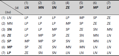
The rule base can be constituted with various sets of rules corresponding to combinations of fuzzy sets on Δu and a. In this example we consider the exhaustive set of rules obtained by taking all possible combinations of fuzzy sets on Δu and a. This is depicted in Table 4.4. This way of tabular representation of a fuzzy rule base is often referred to as a fuzzy associative memory (FAM) table. The entries in the table can be interpreted in the following way: consider the cell at the intersection of row 3 and column 4. Row 3 corresponds to the fuzzy set Small Negative (SN) of Δu and Column 4 corresponds to ZE of acceleration a. The entry in their intersecting cell is SP. Therefore, this entry represents the rule

 

 

Table 4.4. Fuzzy associative memory (FAM) table

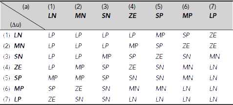
Usually the FAM table may contain some empty cells. An empty cell in the FAM table, if there exists one, indicates the absence of the corresponding rule in the rule base.

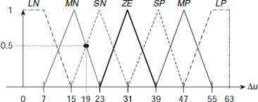
Fig. 4.24.

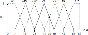
Fig. 4.25.

Let us now work out the output of the controller when the normalized speed difference (Δu) and acceleration (a) are 19 and 35 respectively. It is apparent from Fig. 4.24 that for Δu = 19, all fuzzy sets except MN and SN have zero membership. Similarly, for a = 35 only the fuzzy sets ZE and SP have non-zero memberships. Moreover, it is observed from Fig. 4.24 that at Δu =19 membership to MN is 0.5, Similarly Also, from Fig. 4.25 we get, and Therefore the rules corresponding to cells (MN, ZE), (MN, SP), (SN, ZE), and (SN, SP), cells (2, 4), (2, 5), (3, 4) and (3, 5) of the FAM table, R₂₄, R₂₅, R₃₄, R₃₅ are fired. These rules are

 

R24	:	IF (Δu is MN) AND (a is ZE) THEN (T is MP)
R25	:	IF (Δu is MN) AND (a is SP) THEN (T is SP)
R34	:	IF (Δu is SN) AND (a is ZE) THEN (T is SP)
R35	:	IF (Δu is SN) AND (a is SP) THEN (T is ZE)

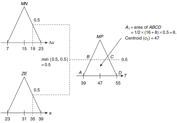
Fig. 4.26. Processing of Rule R₂₄.

Let us employ min function to implement the ‘AND’ operation in the antecedent part of a rule. Accordingly, the processing of R₂₄ is shown in Fig. 4.26. Table 4.5 shows the complete set of areas and their centroids obtained through processing the rules R₂₄, R₂₅, R₃₄, R₃₅.

 

Table 4.5. Areas and centroids

Rule	Area	Centroid
R24	A1 = 6	c1 = 47
R25	A2 = 6	c2 = 39
R34	A3 = 6	c3 = 39
R35	A4 = 6	c4 = 31

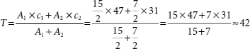
The defuzzified output, according to the CoS method is computed as shown below.

However, to compute T_centroid, the defuzzified output value of throttle control, we have to consider the superimposed region ABCD shown in Fig. 4.27.

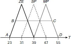
Fig. 4.27. Region for computation of T_centroid.

It is evident from Fig. 4.27 that the region ABCD is a trapezium. The centroid of a trapezium passes through the middle of its parallel sides. Hence, centroid of ABCD is 39. Moreover,

 

Therefore,

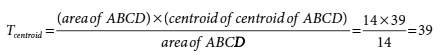
Hence, the value of the throttle control, when computed through the centroid method, too is 39. It may be verified that the defuzzified output, obtained by employing the MoM is also 39. Hence, for this instance of the fuzzy cruise controller we have T_cos = T_centroid = T _MoM = 39.

CHAPTER SUMMARY

The main points of foregoing discussions on fuzzy inference systems are summarized below.

1. A fuzzy inference system (FIS) is a system that transforms a given input to an output with the help of fuzzy logic. The procedure followed by a fuzzy inference system is known as fuzzy inference mechanism, or simply fuzzy inference.
2. The entire fuzzy inference process comprises five steps, fuzzification of the input variables, application of fuzzy operators on the antecedent parts of the rules, evaluation of the fuzzy rules, aggregation of fuzzy sets across the rules, and defuzzification of the resultant aggregate fuzzy set.
3. The first step, fuzzification, determines the degree to which each input belongs to various fuzzy sets through the respective membership function.
4. When the antecedent of a given rule has more than one parts, the appropriate fuzzy operator is applied to obtain a single number representing the result of the entire antecedent. This constitutes the second step of fuzzy inference process.
5. In the third step fuzzy rules are evaluated through some implication process. The output fuzzy set is obtained by reshaping the fuzzy set corresponding to the consequent part of the rule with the help of the number given by the antecedent.
6. The aggregation process takes the truncated membership profiles returned by the implication process as its input, and produces one fuzzy set for each output variable as the output. This constitutes the fourth step of the fuzzy inference process.
7. Defuzzification is the process of converting the aggregate output sets into one crisp number per output variable. This is the fifth, and last, step in a fuzzy inference process.
8. There are various defuzzification methods. The most popular among them are the centroid method, CoS method and the MoM method.

SOLVED PROBLEMS

Problem 4.1 (Fuzzy air conditioner) Consider the fuzzy air conditioner controller discussed in subsection 4.7.1. What is the dial position for ΔT = + 0.5 ?

 

Solution 4.1 The step by step computational process is described below.

(i) Fuzzification Given ΔT = + 0.5, we compute the degree of membership of ΔT with respect to the fuzzy sets LN, MN, ZE, MP, LP using the respective membership profiles depicted in Fig. 4.14. All memberships, except ZE and MP are 0 (Fig. 4.28). For ZE and MP the membership values are 5/6 and 1/6, respectively.

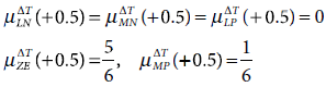
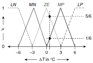
Fig. 4.28. Fuzzy memberships for ΔT = + 0.5

(ii) Rule implication The fuzzy rule base employed is given by

 

	R1 :	IF ΔT is LN THEN D is LP.
	R2 :	IF ΔT is MN THEN D is MP.
	R3 :	IF ΔT is ZE THEN D is ZE.
	R4 :	IF ΔT is MP THEN D is MN.
	R5 :	IF ΔT is LP THEN D is LN.

 

As ZE and MP are the only fuzzy sets having non-zero membership values for ΔT = + 0.5, the fired rules are R₃ and R₄. The rule implication processes are shown in Fig. 4.29 and Fig. 4.30.

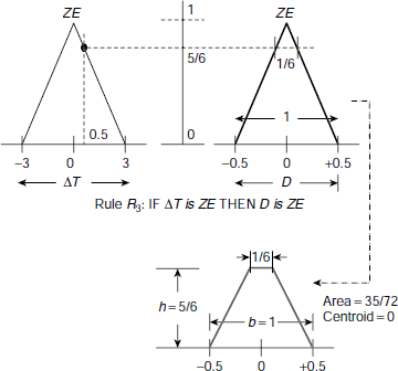
Fig. 4.29. Evaluation of rule R₃.

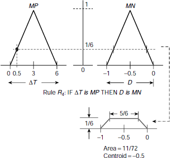
Fig. 4.30. Evaluation of rule R₄.

The implication of the rules R₃ and R₄ results in two regions of areas 35/72 and 11/72 respectively. The corresponding centroids are 0 and – 0.5.

(iii) Aggregation Calculation of the dial value in the CoS method is as follows

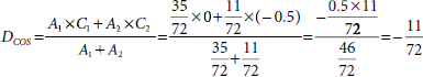
Hence, the output of the fuzzy controller is D = – 11/72.

 

Problem 4.2 (Fuzzy cruise controller) Consider the fuzzy cruise controller discussed in subsection 4.7.2. What will be the value of the throttle control for normalized speed difference (Δu) = 41, and acceleration (a) = 15?

 

Solution 4.2 The step by step computational process is given below.

(i) Fuzzification    Since there are two input parameters, Δu and a, we need to fuzzify both. Considering Δu, we see that the non-zero memberships are and rest of the membership values are all zeros (see Fig. 4.31). Therefore,

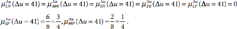
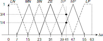
Fig. 4.31.

Similarly, for a, all membership values except MN are zeros (Fig. 4.32), so that

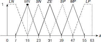
Fig. 4.32.

(ii) Rule implication    The results of the fuzzification phase imply that rules R₅₂ and R₆₂ are fired (see Table 4.6 which is a repetition of Table 4.4 with relevant portions highlighted). Hence we need to process the following fuzzy rules:

 

R52	:	IF (Δu is SP) AND (a is MN) THEN (T is MP)
R62	:	IF (Δu is MP) AND (a is MN) THEN (T is ZE)

 

Table 4.6. Fired Rules in the FAM Table

The rule implication process is graphically shown in Fig. 4.33 and Fig. 4.34.

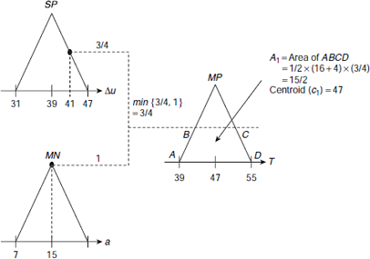
Fig. 4.33. Processing of Rule R₅₂.

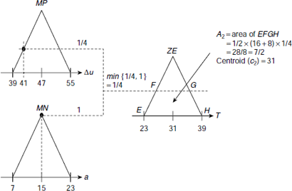
Fig. 4.34. Processing of Rule R₆₂.

The rule implication process yields two trapeziums ABCD and EFGH with areas A₁ = 15/2 and A₂ = 7/2, and centroids c₁ = 47 and c₂ = 31 respectively.

(iii) Aggregation For aggregation, we consider the CoS method only. The calculations are given below.

Hence, the throttle control value will be approximately 42 for normalized speed difference (Δu) = 41, and acceleration (a) = 15.

 

Problem 4.3 (Fuzzy tipper) This problem, popularly known as the tipping problem, concerns the amount of tip to be given to a waiter at a restaurant. It is a typical situation where the principles of fuzzy inference system may be applied successfully. Given a number between 0 and 10 that represents the quality of service at a restaurant (where 10 is excellent), and another number between 0 and 10 that represents the quality of the food at that restaurant (again, 10 is excellent), what should the tip be?

 

Solution 4.3 The starting point is to write down the three golden rules of tipping as given below.

1. If the service is poor or the food is rancid, then tip is cheap.
2. If the service is good, then tip is average.
3. If the service is excellent or the food is delicious, then tip is generous.

The procedure to solve the problem using the relevant MatLab toolbox is being described as a sequence of steps, along with MatLab snapshots.

 

Step 1.

Open Toolboxes → Fuzzy Logic → FIS Editor GUI (Fuzzy).(Fig. 4.35)

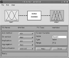
Fig. 4.35. Step 1 of Fuzzy tipper

Step 2.

Open Edit → Add variable → Input. (Normally there is one input and one output available, but we would need two inputs here) (Fig. 4.36)

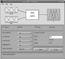
Fig. 4.36

Step 3.	Double click on one of the yellow boxes to go to the Membership Function Editor.
Step 4.	Select Input1 (Service), Input2 (Food) and Output(Tip) to change the variables of the membership functions to suitable values. (Fig. 4.37–4.44)

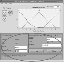
Fig. 4.37

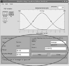
Fig. 4.38

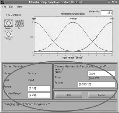
Fig. 4.39

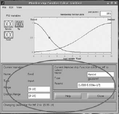
Fig. 4.40

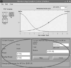
Fig. 4.41

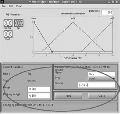
Fig. 4.42

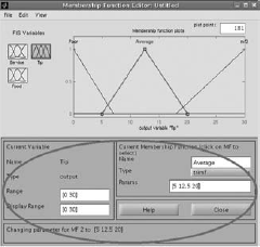
Fig. 4.43

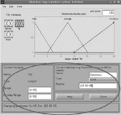
Fig. 4.44

Step 5.	Close the Membership Function Editor to return to FIS Editor.
Step 6.	Double click on the white box in the middle to go to the Rule Editor.
Step 7.	From the options available, add rules as above. (Fig. 4.45)

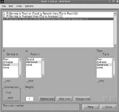
Fig. 4.45

Step 8.	Close the Rule Editor.
Step 9.	Press CTRL + T to export your FIS to Workspace/File or do so from FILE → EXPORT → TO FILE
Step 10.	Now press CTRL + 5 to see the Graphical Rule Viewer where you can vary the input parameter values and see the corresponding output values. (Fig. 4.46)

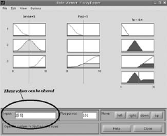
Fig. 4.46

Step 11.

The surface viewer can be invoked by CTRL+6. (Fig. 4.47)

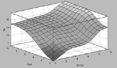
Fig. 4.47

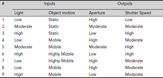
Problem 4.4 (Fuzzy controlled camera) Present day digital cameras have fuzzy controllers to control the aperture and shutter speed of the camera based upon light conditions and the state of motion of the object. Table 4.7 shows the behavior pattern of such a camera. Design a fuzzy inference system to control the aperture and the shutter speed on the basis of light and object motion.

 

Table 4.7. Camera adjustments

Solution 4.4 The MatLab implementation of the fuzzy inference system is described below in a stepwise manner.

Step 1.

Open Toolboxes → Fuzzy Logic → FIS Editor GUI (Fuzzy). (Fig. 4.48)

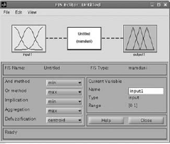
Fig. 4.48

Step 2.	Open Edit → Add variable → Input (Normally there is one input and one output available, but we would need two each here.)
Step 3.	Open Edit → Add variable → Output (To add the second output variable)
Step 4.	Double click on one of the yellow boxes to go to the Membership Function Editor.
Step 5.	Select Input 1 (Light) and change the variables of the membership functions to suitable values. (Fig. 4.49, 4.50, 4.51)

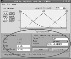
Fig. 4.49

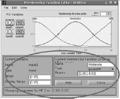
Fig. 4.50

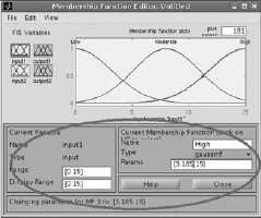
Fig. 4.51

Step 6.

Repeat steps for Input 2 (Object Motion)

Step 7.

Repeat steps for Output 1 (Aperture)

Step 8.

Repeat steps for Output 2 (ShutterSpeed)

Step 9.	Close the Membership Function Editor to return to FIS Editor.
Step 10.	Double click on the white box in the middle to go to the Rule Editor.
Step 11.	From the options available, add rules that appear in the table above.
Step 12.	Close the Rule Editor.
Step 13.	Press CTRL + T to export your FIS to Workspace/File or do so from FILE → EXPORT → TO FILE.
Step 14.	Now press CTRL + 5 to see the Graphical Rule Viewer where you can vary the input parameter values and see the corresponding output values. (Fig. 4.52)

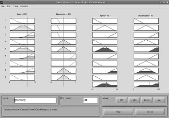
Fig. 4.52

Step 15.

The Surface Viewer can be invoked by CTRL + 6. (Fig. 4.53 and 4.54)

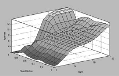
Fig. 4.53

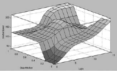
Fig. 4.54

TEST YOUR KNOWLEDGE

4.1 Which of the following is the first step of a fuzzy inference process ?

1. Fuzzification
2. Defuzzification
3. Either (a) or (b)
4. None of the above

4.2 Which of the following is the last step of a fuzzy inference process ?

1. Fuzzification
2. Defuzzification
3. Either (a) or (b)
4. None of the above

4.3 An input to a fuzzy inference system is a

1. A crisp value
2. A linguistic variable
3. A fuzzy set
4. None of the above

4.4 An output of a fuzzy inference system is a

1. A crisp value
2. A linguistic variable
3. A fuzzy set
4. None of the above

4.5 Which of the following is not a defuzzification method?

1. Centroid
2. Centre-of-sums (CoS)
3. Mean-of-maxima (MoM)
4. None of the above

4.6 Fuzzy controllers are built on the basis of

1. Fuzzy Inference Systems
2. Fuzzy Extension Principle
3. Both (a) or (b)
4. None of the above

4.7 Which of the following is used to store a fuzzy rule base of a fuzzy controller?

1. Fuzzy Relation Matrix
2. Fuzzy Associative Memory table
3. Both (a) or (b)
4. None of the above

4.8 Which of the following defuzzification methods is never used in a fuzzy controller?

1. Centroid
2. Center-of-sums (CoS)
3. Mean-of-Maxima (MoM)
4. None of the above

4.9 An empty cell in a Fuzzy Associative Memory (FAM) table indicates

1. An error in the FAM specification
2. A rule that is absent in the rule base
3. Both (a) and (b)
4. None of the above

4.10 Which of the following phases of a fuzzy controller uses the fuzzy rule base?

1. Fuzzification
2. Rule implication
3. Both (a) and (b)
4. None of the above

Answers

4.1 (a)

4.2 (b)

4.3 (a)

4.4 (a)

4.5 (d)

4.6 (a)

4.7 (b)

4.8 (d)

4.9 (b)

4.10 (b)

EXERCISES

4.1 A test is being conducted to ascertain the creative and logical ability of a person. The test has two parts, viz., a reasoning part, and a design part. The score of each part is normalized to the scale of 0–10. There are two output indices, viz., the creative index, and the logical index, both are within the range [0, 1]. The scores of the tests, as well as the outputs, i.e., the creative index, and the logical index, are categorized by the linguistic variables low, medium, and high.

Propose suitable fuzzy set membership functions for each linguistic variable described above. Also propose a fuzzy rule base involving the input and output parameters mentioned above. Design a fuzzy inference system, structurally similar to a fuzzy controller, to find the values of the two indices when the normalized score of the test is given. Find the values of the creative and logical indices for the following sets scores:

 

 

4.2 In Solved Problem No. 4.1 and 4.2, calculate the outputs through centroid method and mean-of-maxima method.

BIBLIOGRAPHY AND HISTORICAL NOTES

Zadeh introduced the idea of a linguistic variable defined as a fuzzy set in 1973. In 1975 Ebrahim Mamdani proposed a fuzzy control system for a steam engine combined with a boiler by employing a set of linguistic control rules provided by human operators from their past experience. In 1987 Takeshi Yamakawa applied fuzzy control, with the help of a set of fuzzy logic chips, in the famous inverted pendulum experiment. In this control problem, a vehicle tries to keep a pole mounted on its top by a hinge upright by moving back and forth. Numerous fuzzy controllers built upon the concepts of fuzzy inference systems were developed for both industrial and consumer applications such as vacuum cleaners, autofocusing camera, air conditioner, low-power refrigerators, dish washer etc. Fuzzy inference systems have been successfully applied to various areas including automatic control, computer vision, expert systems, decision analysis, data classification, and so on. A brief list of the literature in this area is given below.

 

Hirota, K. (ed.) (1993). Industrial Applications of Fuzzy Technology. Springer, Tokyo,

Holmblad L.P. and Ostergaard J.-J. (1982). Control of a cement kiln by fuzzy logic. In Fuzzy Information and Decision Processes, Gupta, M.M. and Sanchez, E. (ed.), pp. 389–399. North-Holland.

Jantzen, J. (2007). Foundations of Fuzzy Control. Wiley.

Mamdani E.H. and Assilian S. (1975). An experiment in linguistic synthesis with a fuzzy logic controller. International Journal of Man-Machine Studies, Vol. 7, pp. 1–13.

Passino, K. M. and Yurkovich, S. (1998). Fuzzy Control. Addison Wesley Longman, Menlo Park, CA.

Santhanam S. and Langari R. (1994). Supervisory fuzzy adaptive control of a binary distillation column. In Proceedings of the 3^rd IEEE International Conference on Fuzzy Systems, Vol. 2, pp. 1063–1068, Orlando, FL.

Tanaka, K. and Wang, H. O. (2001). Fuzzy Control Systems Design and Analysis: a Linear Matrix Inequality Approach. John Wiley and Sons, New York.

Terano, T., Asai, K., and Sugeno, M. (1994). Applied Fuzzy Systems. Academic Press, Boston.

Vadiee, N. (1993). Fuzzy rule based expert systems. In Fuzzy Logic and Control. Prentice-Hall.

Yager, R. and Filev, D. (1994). Essentials of Fuzzy Modeling and Control. John Wiley and Sons, New York.

Yasunobu, S. and Miyamoto, S. (1985). Automatic train operation system by predictive fuzzy control. In Industrial Applications of Fuzzy Control, M. Sugeno (ed.), pp. 1–18. North-Holland.