6
Artificial Neural Networks: Basic Concepts
Key Concepts
Activation, Activation function, Artificial neural network (ANN), Artificial neuron, Axon, Binary sigmoid, Code-book vector, Competitive ANN, Correlation learning, Decision plane, Decision surface, Delta learning, Dendrite, Epoch of learning, Euclidean distance, Exemplar, Extended delta rule, Heaviside function, Heb learning, Hebb rule, Hidden layer, Hopfield network, Hyperbolic tangent function, Identity function, Learning rate, Least-mean square (LMS) learning, Linear separability, Logistic sigmoid, McCulloch–Pitts neural model, Multi-layer feed forward, Neuron, Outstar learning, Parallel relaxation, Pattern, Pattern association, Pattern classification, Perceptron, Perceptron convergence theorem, Perceptron learning, Processing element (PE), Recurrent network, Sigmoid function, Single layer feed forward, Soma, Steepness parameter, Step function, Supervised learning, Synapse, Threshold function, Training vector, Unsupervised learning, Widrow–Hoff rule, Winner takes all, XOR problem
Chapter Outline
6.2 Computation in Terms of Patterns
6.3 The McCulloch–Pitts Neural Model
Artificial neural networks (ANNs) follow a computational paradigm that is inspired by the structure and functionality of the brain. The brain is composed of nearly 100 billion neurons each of which is locally connected to its neighbouring neurons. The biological neuron possesses very elementary signal processing capabilities like summing up the incoming signals and then propagating to its neighbours depending on certain conditions. However the sum total of the parallel and concurrent activities of these 100 billion neurons gives rise to the highly sophisticated, complex, and mysterious phenomenon that we call ‘consciousness’. This chapter provides an overview of the basic concepts of ANNs. Unlike mainstream computation where information is stored as localized bits, an ANN preserves information as weights of interconnections among its processing units. Thus, as in the brain, information in ANNs too resides in a distributed manner, resulting in greater fault tolerance. Moreover, multiple information may be superimposed on the same ANN for storage purpose. We will see that like the human brain, ANNs also perform computation in terms of patterns rather than data. This chapter presents the major artificial neural models, as well as the various ANN architectures and activation functions. The basic learning strategies are also discussed in this chapter.
6.1 INTRODUCTION
Computation is generally perceived as a sequence of operations that processes a set of input data to yield a desired result. The agent that carries out the computation is either an intelligent human being or a typical Von Neumann computer consisting of a processor and a memory, along with the input and the output units (Fig. 6.1). The memory contains both instruction and data. Computation is accomplished by the CPU through a sequence of fetch and execute cycles.
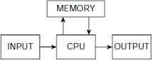
Fig. 6.1. Block diagram of a stored program computer
The sequential fetch and execute model of computation, based on a single-processor stored program digital computer as the hardware platform, has been immensely successful in the history of computers. Its notorious member-crunching and symbol-manipulating capacity has rendered it an indispensable tool for the civilized world. Innumerable applications in everyday activities and other enterprises, e.g. commerce, industry, communication, management, governance, research, entertainment, healthcare, and so on, were developed, are being developed, and shall be developed on the basis of the this model.
However, the power of such a computational model is not unchallenged. There are activities that a normal human being may require a fraction of a second to perform while it would take ages by even the fastest computer. Take, for example, the simple task of recognizing the face of a known person. We do it effortlessly, in spite of the infinite variations due to distance, angle of vision, lighting, posture, distortion due to mood, or emotion of the person concerned, and so on. Occasionally, we recognize a face after a gap of, say, twenty years, even though the face has changed a lot through aging, and has little semblance to its appearance of twenty year ago. This is still very difficult, if not impossible, to achieve for a present day computer.
Where does the power of a human brain, vis-à-vis a stored program digital computer, lie? Perhaps it lies in the fact that we, the human beings, do not think in terms of data as a computer does, but in terms of patterns. When we look at a face, we never think in terms of the pixel values, but perceive the face as a whole, as a pattern. Moreover, the structure of the human brain is drastically different from the Von-Neuman architecture. Instead of one, or a few, processors, the brain consists of 100 billion interconnected cells called the neurons. Individually, a neuron can do no more than some primitive tasks like collecting stimuli from the neighboring neurons and then passing them on to other neighbouring neurons after some elementary processing. But the sum of these simultaneous activities of 100 billion neurons is what we call the human consciousness. Artificial neural network, occasionally abbreviated as ANN, is an alternative model of computation that is inspired by the structure and functionality of the human brain.
6.1.1 The Biological Neuron
The building block of a human brain is the biological neuron. The main parts of the cross-section of a common biological neuron and their functions are shown in Fig. 6.2.
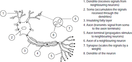
Fig. 6.2. Structure of a biological neuron
It consists of three primary parts, viz., the dendrites, soma, and the axon. The dendrites collect stimuli from the neighbouring neurons and pass it on to soma which is the main body of the cell. The soma accumulates the stimuli received through the dendrites. It ‘fires’ when sufficient stimuli is obtained. When a neuron fires it transmits its own stimulus through the axon. Eventually, this stimulus passes on to the neighboring neurons through the axon terminals. There is a small gap between the end of an axon terminal and the adjacent dendrite of the neighbouring neuron. This gap is called the synapse. A nervous stimulus is an electric impulse. It is transmitted across a synaptic gap by means of electrochemical process.
The synaptic gap has an important role to play in the activities of the nervous system. It scales the input signal by a weight. If the input signal is x, and the synaptic weight is w, then the stimulus that finally reaches the soma due to input x is the product x × w. The significance of the weight w provided by the synaptic gap lies in the fact that this weight, together with other synaptic weights, embody the knowledge stored in the network of neurons. This is in contrast with digital computers where the knowledge is stored as a program in the memory. The salient features of biological neurons are summarized in Table 6.1.
Table 6.1. Salient features of a biological neuron
# | Feature |
|---|---|
1 | The body of the neuron is called the soma that acts as a processing element to receive numerous signals through the dendrites simultaneously. |
2 | The strengths of the incoming signals are modified by the synaptic gaps. |
3 | The role of the soma, i.e., the processing element of a neuron, is simple. It sums up the weighted input signals and if the sum is sufficiently high, it transmits an output signal through the axon. The output signal reaches the receiving neurons in the neighbourhood through the axon terminals. |
4 | The weight factors provided by the synaptic gaps are modified over time and experience. This phenomenon, perhaps, accounts for development of skills through practice, or loss of memory due to infrequent recall of stored information. |
6.1.2 The Artificial Neuron
An artificial neuron is a computational model based on the structure and functionality of a biological neuron. It consists of a processing element, a number of inputs and weighted edges connecting each input to the processing element (Fig. 6.3). A processing unit is usually represented by a circle, as indicated by the unit Y in Fig. 6.3. However, the input units are shown with boxes to distinguish them from the processing units of the neuron. This convention is followed throughout this book. An artificial neuron may consist of m number of input units X1, X2, …, Xm. In Fig. 6.3 the corresponding input signals are shown as x1, x2, , xm, and y_out is the output signal of the processing unit Y.
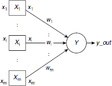
Fig. 6.3 Structure of an artificial neuron
The notations used in Fig. 6.3 are summarized in Table 6.2. These notational conventions are followed throughout this text unless otherwise stated.
Table 6.2. Notational convention
Symbol Used | Description |
|---|---|
Xi | The ith input unit. |
Y | The output unit. In case there are more than one output units, the jth output unit is denoted as Yj. |
xi | Signal to the input unit Xi. This signal is transmitted to the output unit Y scaled by the weight wi. |
wi | The weight associated with the interconnection between input unit Xi and the output unit Y. In case there are more than one output units, wij denotes the weight between input unit Xi and the jth output unit Yj. |
y_in | The total (or net) input to the output unit Y. It is the algebraic sum of all weighted inputs to Y. |
y_out | Signal transmitted by the output unit Y. It is known as the activation of Y. |
The net input y_in to the processing element Y is obtained as
If there are more than one output units, then the net input to the jth output unit Yj, denoted as y_inj, is given by
The weight wi associated with the input Xi may be positive, or negative. A positive weight wi means the corresponding input Xi has an excitatory effect on Y. If, however, wi is negative then the input Xi is said to have an inhibitory effect on Y. The output signal transmitted by Y is a function of the net input y_in. Hence,
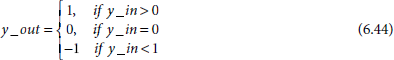
In its simplest form f(.) is a step function. A binary step function for the output unit is defined as
Taking Equation 6.1 into consideration we get
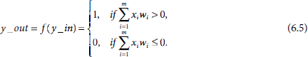
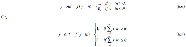
When a non-zero threshold θ is used Equations 6.4 and 6.5 take the forms
The function f(.) is known as the activation function of the neuron, and the output y_out is referred to as the activation of Y. Various activation functions are discussed in later parts of this chapter.
The structure of an artificial neuron is simple, like its biological counterpart. It’s processing power is also very limited. However, a network of artificial neurons, popularly known as ANN has wonderful capacities. The computational power of ANNs is explored in the subsequent chapters with greater details.
6.1.3 Characteristics of the Brain
Since brain is the source of inspiration, as well as the model that ANNs like to follow and achieve, it is worthwhile to ponder over the characteristics of a brain as a computing agent. The most striking feature of a brain is its extremely parallel and decentralized architecture. It consists of more or less 100 billion neurons interconnected among them. The interconnections are local in the sense that each neuron is connected to its neighbours but not to a neuron far away. There is practically no centralized control in a brain. The neurons act on the basis of local information. These neurons function in parallel mode and concurrently. Apparently the brain is very slow compared to the present day computers. This is due to the fact that neurons operate at milliseconds range while the modern VLSI microchip process signals at nanosecond scale of time. The power of the brain lies not in the signal processing speed of its neuron but in the parallel and concurrent activities of 100 billion neurons. Another fascinating fact about the brain is its fault tolerance capability. As the knowledge is stored inside the brain in a distributed manner it can restore knowledge even when a portion of the brain is damaged. A summary of the essential features of a brain is presented in Table 6.3.
Table 6.3. Essential features of a brain
# | Aspect | Description |
|---|---|---|
1 | Architecture | The average human brain consists of about 100 billion neurons. There are nearly 1015 number of interconnections among these neurons. Hence the brain’s architecture is highly connected. |
2 | Mode of operation | The brain operates in extreme parallel mode. This is in sharp contrast with the present day computers which are essentially single-processor machines. The power of the brain lies in the simultaneous activities of 100 billion neurons and their interactions. |
3 | Speed | Very slow, and also very fast. Very slow in the sense that neurons operate at milliseconds range which is miserably slow compared to the speed of present day VLSI chips that operate at nanoseconds range. So computers are tremendously fast and flawless in number crunching and data processing tasks compared to human beings. Still the brain can perform activities in split-seconds (e.g., converse in natural language, carry out common sense reasoning, interpret a visual scenery, etc.) which a modern supercomputer may take ages to carryout. |
4 | Fault tolerance | The brain is highly fault tolerant. Knowledge is stored within the brain in a distributed manner. Consequently, if a portion of the brain is damaged, it can still go on functioning by retrieving or regenerating the lost knowledge from the remaining neurons. |
5 | Storage mechanism | The brain stores information as strengths of the interconnections among the neurons. This accounts for the adaptability of the brain. New information can be added by adjusting the weights without destroying the already stored information. |
6 | Control | There is no global control in the brain. A neuron acts on local information available with its neighbouring neurons. The neurons pass on the results of processing only to the neurons adjacent to them. |
6.2 COMPUTATION IN TERMS OF PATTERNS
It was observed earlier in this chapter that the brain perceives the physical world in terms of patterns, rather than data. Since ANNs are inspired by the brain, both structurally and behaviourally, it is worthwhile to consider the nature of pattern-oriented computation vis-a-vis computation on the basis of stored program. Two fundamental operations relating to patterns, pattern classification and pattern association, are explained in this subsection with the help of simple illustrative examples.
6.2.1 Pattern Classification
Classification is the process of identifying the class to which a given pattern belongs. For example, let us consider the set S of all 3-bit patterns. We may divide the patterns of S into two classes A and B where A is the class of all patterns having more 0s than 1s and B the converse. Therefore
S = {000, 001, 010, 011, 100, 101, 110, 111}
A = {000, 001, 010, 100}
B = {011, 101, 110, 111}
Now, given an arbitrary 3-bit pattern, the classification problem here is to decide whether it belongs to the class A, or class B. In other words, we have to establish the mapping shown in Fig. 6.4.
The simplest way to achieve this is to execute a table look-up procedure, as shown in Fig. 6.5(a). All we have to do is to find the appropriate row in the table corresponding to the given pattern and read the class name to which it belongs. However, creation and storage of the table becomes impractical as the volume of stored patterns increases. In practice, we may have to deal with billions of multidimensional patterns.
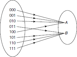
Fig. 6.4. Classification of 3-bit patterns based on the number of 0s and 1s.
Fig. 6.5(b) presents a conventional computer program to perform this task. The program is written in a pseudo-language. The technique is to count the number of 0s and 1s in the given patterns and store them in the local variables n0 and n1. Then depending on whether n0 > n1 or n0 < n1 the program returns the class name A or B respectively. The algorithm has a time complexity of O(nb) where nb is the number of bits in the given pattern.
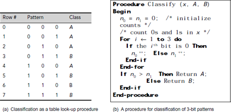
Fig. 6.5. Two methods for classification of 3-bit patterns
Is it possible to solve the problem in a different way? Fig. 6.6 shows an artificial neuron with three inputs x1, x2, x3 connected to a processing element Y through the weight factors as shown in the figure. It is a simplified version of a neural model called perception, proposed by Rosenblatt in 1962.
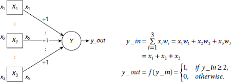
Fig. 6.6 An artificial neuron to classify 3-bit binary patterns based on the number of 0s and 1s
The weights w1, w2, w3 associated with the interconnection paths from the inputs x1, x2, x3 to Y are chosen in a way that the net input y_in to Y is greater than or equal to 2 when there are two or more 1s among x1, x2, x3. The activation y_out then becomes 1, indicating that the patterns belongs to the class B. On the other hand, when there are more 0s than 1s, the net (total) input ![]() so that the output signal, the activation, is y_out = 0. This implies that the given pattern belongs to the class A. Time complexity of this method is O(1) because the inputs are fed to the processing element parallely.
so that the output signal, the activation, is y_out = 0. This implies that the given pattern belongs to the class A. Time complexity of this method is O(1) because the inputs are fed to the processing element parallely.
An alternative arrangement of two output nodes Y1 and Y2 to solve the same classification problem is shown in Fig. 6.7. Here both the units Y1 and Y2 are connected to the same inputs x1, x2, x3 and these units explicitly correspond to the classes A and B respectively. If the input pattern belongs to the class A then Y1 fires (i.e., computes the activation as y_out1 = 1), otherwise, unit Y2 fires. Y1 and Y2 never fire simultaneously.
It should be noted that Fig. 6.5(a) and 6.5(b) presents the classification knowledge in the form of an algorithm. On the other hand, the ANN counterpart of the concerned classification task embodies the same knowledge in the form of certain interconnection weights and the activation functions. If we change the weights, or the activation functions f(y_in), the capability of the ANN changes accordingly.
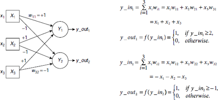
Fig. 6.7. Classification of 3-bit patterns with two output units
6.2.2 Pattern Association
Associating an input pattern with one among several patterns already stored in memory, in case such a mapping exists, is an act that we, the human beings, carry out effortlessly in our daily life. A person, with his eyes closed, can visualize a rose by its fragrance. How does it happen? It seems that various odours are already stored in our memory. When we smell an odour, our brain tries to map this sensation to its stored source. It returns the nearest match and this correspond to recognizing the odour, or the sensation in general. However, in case there is no match between the input sensation and any of the stored patterns – we fail to associate the input, or, to be more precise, we conclude that the input is unknown to us.
Given an input pattern, and a set of patterns already stored in the memory, finding the closest match of the input pattern among the stored patterns and returning it as the output, is known as pattern association. The basic concept of pattern association is explained below with the help of a simple illustrative example. The example is inspired by Hopfield network [1982] which is discussed later in greater details.
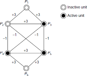
Fig. 6.8. A network for pattern recognition
Let us consider a network of six processing elements (PEs) or units as shown in Fig. 6.8. The essential features of the network are described below.
- PE states At any instant, a unit may either be in an active or an inactive state. Moreover, depending on the circumstances, the state of a unit may change from active to inactive, and vice versa. In Fig. 6.8 an active unit is shown with a black circle and an inactive unit is indicated by a hollow circle.
- Interconnections All interconnections are bidirectional. Magnitude of the weight associated with an interconnection gives the strength of influence the connected units play on each other.
- Signed weights A negative weight implies that the corresponding units tend to inhibit, or deactivate, each other. Similarly, positively interconnected units tend to activate each other.
- Initialization The network is initialized by making certain units active and keeping others inactive. The initial combination of active and inactive units is considered as the input pattern. After initialization, the network passes through a number of transformations. The transformations take place according to the rules described below.
- Transformations At each stage during the sequence of transformations, the next state of every unit Pi, i = 1, …, 6, is determined. The next state of a unit Pi is obtained by considering all active neighbours of Pi and taking the algebraic sum of the weights of the paths between Pi and the neighbouring active units. If the sum is greater than 0, then Pi becomes active for the next phase. Otherwise it becomes inactive. The state of a unit without any active unit in its neighbourhood remains unaltered. This process is known as parallel relaxation.
For example, let the network be initialized with the pattern shown in Fig. 6.9(a). Initially, all units except P2 and P5 are inactive. To find the state of P1 in the next instant, we look for the active neighbours of P1 and find that P2 is the only active unit connected to P1 through an interconnection link of weight +3. Hence P1 becomes active in the next instant. Similarly, for P3, both P2 and P5 are active units in its neighbourhood. The sum of the corresponding weights is w23 + w35 = +3 −1 = +2. Hence P3 also becomes active. However P2 itself becomes inactive because the only active unit in its vicinity, P5, is connected to it through a negatively weighted link. Table 6.4 shows the details of computations for transformation of the network from Fig. 6.9(a) to Fig. 6.9(b). The configuration of Fig. 6.9(b) is not stable. The network further transforms itself from Fig. 6.9(b) to Fig. 6.9(c), which is a stable state. Therefore, we can say that the given network associates the pattern shown in Fig. 6.9(a) to that shown in Fig. 6.9(c).
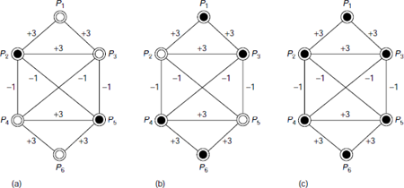
Fig. 6.9. Pattern association through parallel relaxation
A little investigation reveals that the given network has three non-trivial stable states as shown in Fig. 6.10(a)-(c). The trivial state is that where all units are inactive. It can be easily verified that if one or more of the units P1, P2, P3 is/are active initially while the rest, P4, P5, P6 are inactive, the network converges to the pattern shown in Fig. 6.10(a). Similarly, the pattern of Fig. 6.10(b) is associated with any input pattern where at least one unit of the group {P4, P5, P6} is/are active. Finally, an input pattern having active units from both the groups {P1, P2, P3} and {P4, P5, P6} would associate to with the patterned depicted in Fig. 6.10(c). Hence, the given network may be thought of as storing three non-trivial patterns as discussed above. Such networks are also referred to as associative memories, or content-addressable memories.
Table 6.4. Computation of parallel relaxation on Fig. 6.9 (a)
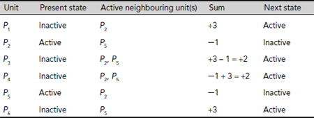
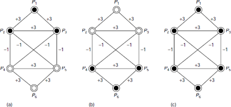
Fig. 6.10. Non-trivial patterns stored in a Hopfield network
6.3 THE McCULLOCH–PITTS NEURAL MODEL
The earliest artificial neural model was proposed by McCulloch and Pitts in 1943. Fig. 6.11 depicts its structure. It consists of a number of input units connected to a single output unit. The interconnecting links are unidirectional. There are two kinds of inputs, namely, excitatory inputs and inhibitory inputs. The salient features of a McCulloch and Pitts neural net are summarized in Table 6.5.
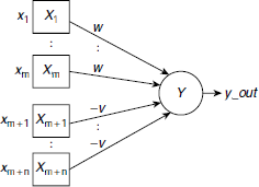
Fig. 6.11. Structure of a McCulloch-Pitts neuron
Table 6.5. Salient features of McCulloch-Pitts artificial neuron
1 | There are two kinds of input units, excitatory, and inhibitory. In Fig. 6.11 the excitatory inputs are shown as inputs X1, …, Xm and the inhibitory inputs are Xm+1, …, Xm+n. The excitatory inputs are connected to the output unit through positively weighted links. Inhibitory inputs have negative weights on their connecting paths to the output unit. |
2 | All excitatory weights have the same positive magnitude w and all inhibitory weights have the same negative magnitude −v. |
3 | The activation y_out = f(y_in) is binary, i.e., either 1 (in case the neuron fires), or 0 (in case the neuron does not fire). |
4 | The activation function is a binary step function. It is 1 if the net input y_in is greater than or equal to a given threshold value θ, and 0 otherwise. |
5 | The inhibition is absolute. A single inhibitory input should prevent the neuron from firing irrespective of the number of active excitatory inputs. |
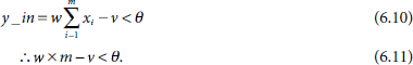
The net input y_in to the neuron Y is given by
If θ be the threshold value, then the activation of Y, i.e., y_out, is obtained as
To ensure absolute inhibition, y_in should be less than the threshold even when a single inhibitory input is on while none of the excitatory inputs are of. Assuming that the inputs are binary, i.e., 0 or 1, the criterion of absolute inhibition requires
Simple McCulloch-Pitts neutrons can be designed to perform conventional logical operations. For this purpose one has to select the appropriate number of inputs, the inter connection weights and the appropriate activation function. A number of such logic-performing McCulloch-Pitts neural nets are presented below as illustrative examples.
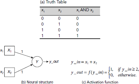
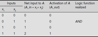
Fig. 6.12. A McCulloch-Pitts neuron to implement logical AND operation
Fig. 6.12 shows a McCulloch-Pitts neuron to perform the logical AND operation. It should be noted that all inputs in Fig. 6.12(b) are excitatory. No inhibitory input is required to implement the logical AND operation. The interconnection weights and the activation functions are so chosen that the output is 1 if and only if both the inputs are 1, otherwise it is 0.
Example 6.2 (Implementation of logical OR with McCulloch-Pitts neural model)
The McCulloch-Pitts neuron to perform logical OR operation is shown in Fig. 6.13. It is obvious from the figure that the neuron outputs a 1 whenever there is at least one 1 at its inputs. The neuron is structurally identical to the AND-performing neuron. Only the activation function is changed appropriately so that the desired functionality is ensured.
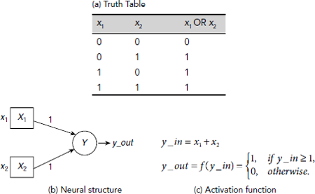
Fig. 6.13. A McCulloch-Pitts Neuron to implement logical OR operation
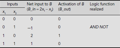
Example 6.3 (Implementation of logical AND-NOT with McCulloch-Pitts neural model)
The logical AND-NOT operation is symbolically expressed as x1. x2´, or x1 AND (NOT x2). It produces a 1 at the output only when x1 is 1 and x2 is 0. The McCulloch-Pitts neuron to perform this operation is shown in Fig. 6.14. The inhibitory effect of x2 is implemented by attaching a negative weight to the path between x2 and Y. The arrangement ensures that the output is 1 only when x1 = 1 and x2 = 0. For all other combinations of x1 and x2 the output is 0.
Example 6.4 (Implementation of logical XOR with McCulloch-Pitts neural model)
As in digital logic design, simple McCulloch-Pitts neurons performing basic logical operations can be combined together to implement complex logic functions. As an example, Fig. 6.15 shows the implementation of the XOR function with two AND-NOT operations. Unlike the previous examples, here we had to implement the function with the help of a network of neurons, rather them a single neuron. Moreover, the neurons are placed at various levels so that the outputs from a lower level are fed as inputs to the next level of neurons. All the three processing elements, Y1, Y2, and Z, have the same activation function as described in Fig. 6.15 (c). The net_in is the net input to a processing element. For example, net-in for Y1, is y_in1 = x1 − x2. The same for the units Y2 and Z are y_in2 = − x1 + x2, and z_in = y_out1 + y_out2 respectively, where y_out1 and y_out2 are the respective activations of the units Y1 and Y2.
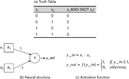
Fig. 6.14. Logical AND-NOT operation with a McCulloch-Pitts neuron
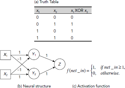
Fig. 6.15. McCulloch-Pitts neural network to implement logical XOR operation
Consider the McCulloch-Pitts neural network shown in Fig. 6.16. All the units, except those at the input level, have the activation function
What are the responses of the output unit Z with respect to various input combinations? We assume the inputs are binary. What logical function the whole network realizes?

Fig. 6.16. A McCulloch-Pitts neural network
Let us first compute the responses of the intermediate units A and B. The responses of the output unit Z will be determined subsequently.
a) Responses of unit A
b) Responses of unit B
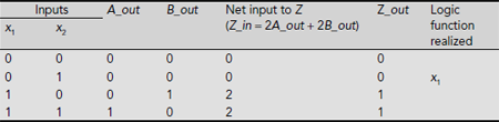
Hence the logic function realized by the whole network is f(x1, x2) = x1.
6.4 THE PERCEPTRON
The perceptron is one of the earliest neural network models proposed by Rosenblatt in 1962. Early neural network enthusiasts were very fond of the perceptron due to its simple structure, pattern classifying behaviour, and learning ability. As far as the study of neural networks is concerned the perceptron is a very good starting point. This section provides the fundamental features of perceptron, namely, its structure, capability, limitations, and clues to overcome the limitations.

Fig. 6.17. Structure of a perceptron
6.4.1 The Structure
The structure of a perceptron is essentially same as that presented in subsection 6.1.2 and is shown here as Fig. 6.17(a). It consists of a number of input units X1, …, Xm and a processing unit Y. The connecting path from input Xi to Y is unidirectional and has a weight wi. The weight wi is positive if xi is an excitatory input and is negative if it is inhibitive. The net input y_in of the perceptron to Y is the algebraic sum of the weighted inputs.
Equation 6.12 can be expressed concisely in matrix notation as given in Equations 6.13(a) and 6.13(b).
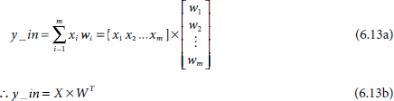
Here X = [x1, …, xm] and W = [w1, …, wm] are the input and the weight vectors.
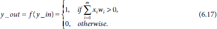
The perceptron sends an output 1 if the net input y_in is greater than a predefined adjustable threshold value θ, otherwise it sends output 0. Hence, the activation function of a perceptron is given by Equation 6.6, repeated below.
Therefore, in matrix notation,
It is customary to include the adjustable threshold θ as an additional weight w0. This additional weight w0 is attached to an input X0 which is permanently maintained as 1. The modified structure inclusive of the adjustable weight w0 and the additional input unit X0 replacing the threshold θ is shown in Fig. 6.17(b). The expressions for the net input y_in and the activation y_out of the perceptron now take the forms
and
The following points should be noted regarding the structure of a perceptron.
- The inputs to a perceptron x0, …, xm are real values.
- The output is binary (0, or 1).
- The perceptron itself is the totality of the input units, the weights, the summation processor, activation function, and the adjustable threshold value.
The perceptron acts as the basic ANN structure for pattern classification. The next subsection describes the capabilities of a perceptron as a pattern classifier.
6.4.2 Linear Separability
As mentioned earlier, perceptrons have the capacity to classify patterns. However, this pattern-classifying capacity is not unconditional. In this subsection, we investigate the criteria for a perceptron to act properly as a pattern classifier.
Let us consider, for example, two sets of points on a two-dimensional Cartesian plane A = {a, b, c} = {(–1, 3), (1, 2), (3, 3)}, and B = {p, q, r} = {(0, –1), (2, 1), (3, 0)}. These points are shown in Fig. 6.18. The points belonging to the set A, or B are indicated with white, and black dots respectively.
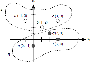
Fig. 6.18. A classification problem consisting for two sets of patterns A, and B.
We look for a classifier that can take an input pattern of the form (x1, x2) and decide to which class, A or B, the pattern belongs. A perceptron that carries out this job is shown in Fig. 6.19. The weights of the perceptron are carefully chosen so that the desired behaviour is achieved. However, we shall see that the weights need not to be chosen, but be learnt by the perceptron. The activation y_out = 1 if the input pattern belongs to class A, and y_out = 0 if it belongs to class B. Table 6.6 verifies that the perceptron shown in Fig. 6.19 can solve the classification problem posed in Fig. 6.18.
In fact, the pattern classifying capability of a perceptron is determined by the equations
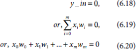
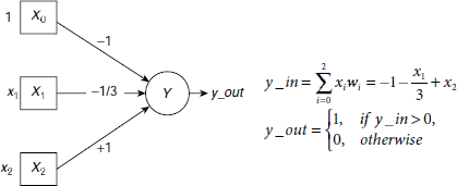
Fig. 6.19. A perceptron to solve the classification problem shown in Fig. 6.17.
Table 6.6. Details of classification of patterns between sets A and B
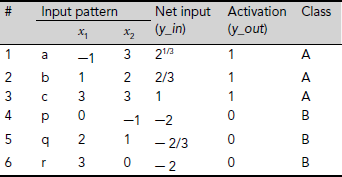
Applying Equations 6.18–6.20 for the perceptron under consideration we get
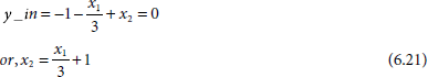
Equation 6.21 represents a straight line that separates the given sets of patterns A and B (Fig. 6.20). For two dimensional patterns of the form (x1, x2) the equation in terms of the weights looks like
Similarly, when the patterns are 3-dimensional and of the form (x1, x2, x3), Equation 6.20 would be
which represents a plane surface. In general, for n-dimensional patterns, Equation 6.20 represents a hyperplane in the corresponding n-dimensional hyperspace. Such a plane for a given perceptron capable of solving certain classification problem is known as a decision plane, or more generally, the decision surface.
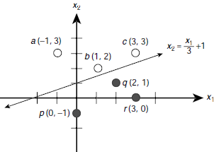
Fig. 6.20. Linearly separable set of patterns
A linearly separable set of patterns is one that can be completely partitioned by a decision plane into two classes. The nice thing about the perceptrons is, for a given set of linearly separable patterns, it is always possible to find a perceptron that solves the corresponding classification problem. The only thing we have to ensure is to find the appropriate combination of values for the weights w0, w1, …, wm. This is achieved through a process called learning or training by a perceptron. The famous perceptron convergence theorem (Rosenblatt [1962]) states that a perceptron is guaranteed to learn the appropriate values of the weights w0, w1, …, wm so that the given a set of linearly separable patterns are properly classified by the perceptron. There are various techniques for training neural networks. A brief overview of these techniques is presented in the later parts of this chapter.
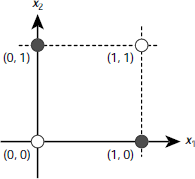
Fig. 6.21. The XOR problem offers patterns that are not linearly separable
6.4.3 The XOR Problem
Real life classification problems, however, rarely offer such well-behaved linearly separable data as required by a perceptron. Minsky and Papert [1969] showed that no perceptron can learn to compute even a trivial function like a two bit XOR. The reason is, there is no single straight line that may separate the 1-producing patterns {(0, 1), (1, 0)} from the patterns 0-producing patterns {(0, 0), (1, 1)}. This is illustrated in Fig. 6.21. Is it possible to overcome this limitation? If yes, then how? There are two ways. One of them is to draw a curved decision surface between the two sets of patterns as shown in Fig. 6.22(a) or 6.22(b). However, perceptron cannot model any curved surface.
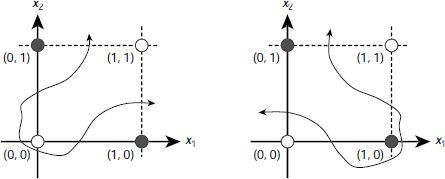
Fig. 6.22. Solving the XOR problem with curved decision surface
The other way is to employ two, instead of one, decision lines. The first line isolates the point (1, 1) from the other three points, viz., (0, 0), (0, 1), and (1, 0). The second line partitions {(0, 0), (0, 1), (1, 0)} into the classes {(0, 1), (1, 0)} and {(0, 0)}. The technique is shown is Fig. 6.23. Fig. 6.23(b) shows another pair of lines that solve the problem in a different way.
Using this idea, it is possible design a multi-layered perceptron to solve the XOR problem. Such a multilayered perceptron is shown in Fig. 6.24. Here the first perceptron Y fires only when the input is (1, 1). But this sends a large inhibitive signal of magnitude –2.0 to the second perceptron Z so that the excitatory signals from x1 and x2 to Z are overpowered. As a result the net input to Z attains a negative value and the perceptron fails to fire. On the other hand, the remaining three input patterns, (0, 0), (0, 1), and (1, 0), for which perceptron Y does not influence Z, are processed by Z in the desired way.

Fig. 6.23. Solving the XOR problem with two decision lines
Hence, the arrangement of perceptrons shown in Fig. 6.24 successfully classifies the patterns posed by the XOR problem. The critical point is, the perceptron convergence theorem is no longer applicable to multilayer perceptrons. The perceptron learning algorithm can adjust the weights of the interconnections between the inputs and the processing element, but not between the processing elements of two different perceptrons. The weight –2.0 in Fig. 6.24 is decided through observation and analysis, not by training.
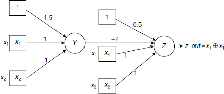
Fig. 6.24. A multi-layer perceptron to solve the XOR problem
6.5 NEURAL NETWORK ARCHITECTURES
An ANN consists of a number of artificial neurons connected among themselves in certain ways. Sometime these neurons are arranged in layers, with interconnections across the layers. The network may, or may not, be fully connected. Moreover, the nature of the interconnection paths also varies. They are either unidirectional, or bidirectional. The topology of an ANN, together with the nature of its interconnection paths, is generally referred to as its architecture. This section presents an overview of the major ANN architectures.
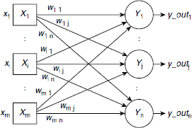
Fig. 6.25. Structure of a single-layer feed forward ANN
6.5.1 Single Layer Feed Forward ANNs
Single layer feed forward is perhaps the simplest ANN architecture. As shown in Fig. 6.25, it consists of an array of input neurons connected to an array of output neurons. Since the input neurons do not exercise any processing power, but simply forward the input signals to the subsequent neurons, they are not considered to constitute a layer. Hence, the only layer in the ANN shown in Fig. 6.25 is composed of the output neurons Y1, …, Yn.
The ANN shown in Fig. 6.25 consists of m inputs X1, …, Xm and n outputs Y1, …, Yn. The signal transmitted by input Xi is denoted as xi. Each input Xi is connected to each output Yj. The weight associated with the path between Xi and Yj is denoted as wij. The interconnection paths are unidirectional and are directed from the input units to the output units.
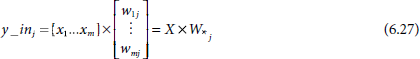
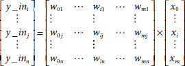
The net input y_in1 to the output unit Y1 is given by
In vector notation, Equation 6.24 can be expressed as
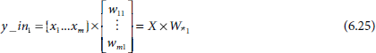
where X = [x1 … xm] is the input vector of the input signals and W*1 is the first column of the weight matrix
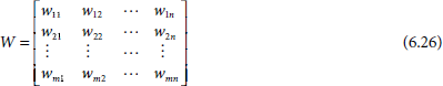
In general, the net input y_inj to the output unit Yj is given by
If Y_in denotes the vector for the net inputs to the array of output units
then the net input to the entire array of output units can be expressed concisely in matrix notation as
The signals transmitted by the output units, of course, depend on the nature of the activation functions. There are various kinds of activation functions and these are discussed in greater details in the next subsection. The basic single layer feed forward network architecture presented in this section has its own variations. For example, in some cases the network may allow interconnections among the input or output units themselves. These will be discussed later in greater details.
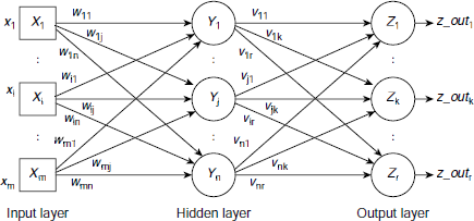
Fig. 6.26. A multi-layer feed forward network with one hidden layer
6.5.2 Multilayer Feed Forward ANNs
A multilayer feed forward net is similar to single layer feed forward net except that there is (are) one or more additional layer(s) of processing units between the input and the output layers. Such additional layers are called the hidden layers of the network. Fig. 6.26 shows the architecture of a multi-layer feed forward neural net with one hidden layer.
The expressions for the net inputs to the hidden layer units and the output units are obtained as
where
X = [x1, x2, …, xm], X is the input vector,
Y_in = [y_in1, y_in2, …, y_inn], is the net input vector to the hidden layer,
Z_in = [z_in1, z_in2, …, z_inr], is the net input vector to the output layer,
Y_out = [y_out1, y_out2, …, y_outn], is the output vector from the hidden layer,
W and V are the weight matrices for the interconnections between the input layer, hidden layer, and output layer respectively.
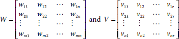
Fig. 6.26 shows the structure of a multi-layered feed forward net with one hidden layer. Obviously, it is possible to include more than one hidden layers in such networks.
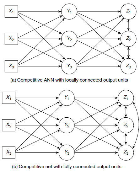
Fig. 6.27. Competitive ANN architectures
6.5.3 Competitive Network
Competitive networks are structurally similar to single layer feed forward nets. However, the output units of a competitive neural net are connected among themselves, usually through negative weights. Fig. 6.27(a) and 6.27(b) show two kinds of competitive networks. In Fig. 6.27(a), the output units are connected only to their respective neighbours, whereas the network of Fig. 6.27(b) shows a competitive network whose output units are fully connected. For a given input pattern, the output units of a competitive network tend to compete among themselves to represent that input. Thus the name competitive network.
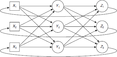
Fig. 6.28 A recurrent network with feedback paths from the output layer to the input layer
6.5.4 Recurrent Networks
In a feed forward network signals flow in one direction only and that is from the input layer towards the output layer through the hidden layers, if any. Such networks do not have any feedback loop. In contrast, a recurrent network allows feedback loops. A typical recurrent network architecture is shown in Fig. 6.28. Fig. 6.29(a) shows a fully connected recurrent network. Such networks contain a bidirectional path between every pair of processing elements. Moreover, a recurrent network may contain self loops, as shown in Fig. 6.29(b).
6.6 ACTIVATION FUNCTIONS
The output from a processing unit is termed as its activation. Activation of a processing unit is a function of the net input to the processing unit. The function that maps the net input value to the output signal value, i.e., the activation, is known as the activation function of the unit. Some common activation functions are presented below.
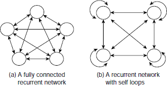
Fig. 6.29. Recurrent network architectures
6.6.1 Identity Function
The simplest activation function is the identity function that passes on the incoming signal as the outgoing signal without any change. Therefore, the identity activation function g(x) is defined as
Fig. 6.30 shows the form of the identity function graphically. Usually, the units of the input layer employ the identity function for their activation. This is because in ANN, the role of an input unit is to forward the incoming signal as it is to the units in the next layer through the respective weighted paths.
6.6.2 Step Function
Another frequently used activation function is the step function. The basic step function produces a 1 or 0 depending on whether the net input is greater than 0 or otherwise. This is the only activation function we have used so far in this text. Mathematically the step function is defined as follows.
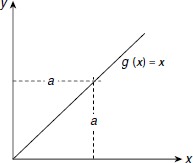
Fig. 6.30. The identity activation function
Fig. 6.31(a) shows the shape of the basic step function graphically. Occasionally, instead of 0 a non-zero threshold value θ is used. This is known as the threshold function and is defined as
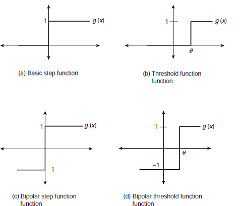
Fig. 6.31. Step functions
The shape of the threshold function is shown in Fig. 6.31(b). The step function is also known as the heaviside function. The step functions discussed so far are binary step functions since they always evaluates to 0 or 1.
Occasionally, it is more convenient to work with bipolar data, –1 and +1, than the binary data. If a signal of value 0 is sent through a weighted path, the information contained in the interconnection weight is lost as it is multiplied by 0. To overcome this problem, the binary input is converted to bipolar form and then a suitable bipolar activation function is employed. Accordingly, binary step functions have their bipolar versions. The output of a bipolar step function is –1, or +1, not 0, or 1. The bipolar step function and threshold function are shown in Fig. 6.31(c) and (d) respectively. They are defined as follows.
Bipolar step function:
Bipolar threshold function:
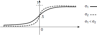
Fig. 6.32. Binary Sigmoid function
6.6.3 The Sigmoid Function
As the step function is not continuous it is not differentiable. Some ANN training algorithm requires that the activation function be continuous and differentiable. The step function is not suitable for such cases. Sigmoid functions have the nice property that they can approximate the step function to the desired extent without losing its differentiability. Binary sigmoid, also referred to as the logistic sigmoid, is defined by Equation 6.36.
The parameter σ in Equation 6.36 is known as the steepness parameter. The shape of the sigmoid function is shown in Fig. 6.32. The transition from 0 to 1 could be made as steep as desired by increasing the value of σ to appropriate extent.
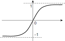
Fig. 6.33. Bipolar Sigmoid function
The first derivative of g(x), denoted by g′(x) is expressed as
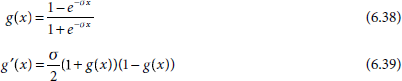
Depending on the requirement, the binary sigmoid function can be scaled to any range of values appropriate for a given application. The most widely used range is from –1 to +1, and the corresponding sigmoid function is referred to as the bipolar sigmoid function. The formulae for the bipolar sigmoid function and its first derivative are given below as Equations 6.38 and 6.39 respectively. Fig. 6.33 presents its form graphically.
6.6.4 Hyperbolic Tangent Function
Another bipolar activation function that is widely employed in ANN applications is the hyperbolic tangent function. The function, as well as its first derivative, are expressed by Equations 6.40 and 6.41 respectively.
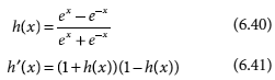
The hyperbolic tangent function is closely related to the bipolar sigmoid function. When the input data is binary and not continuously valued in the range from 0 to 1, they are generally converted to bipolar form and then a bipolar sigmoid or hyperbolic tangent activation function is applied on them by the processing units.
6.7 LEARNING BY NEURAL NETS
An ANN is characterized by three entities, it’s architecture, activation function, and the learning technique. Learning by an ANN refers to the process of finding the appropriate set of weights of the interconnections so that the ANN attains the ability to perform the designated task. The process is also referred to as training the ANN.
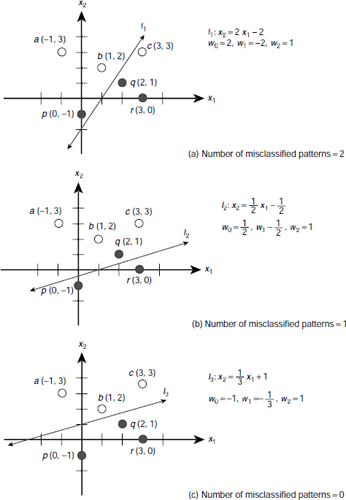
Fig. 6.34. Learning a pattern classification task by a perceptron
Let us, once again, consider the classification problem posed in Section 6.4.2 (Fig. 6.18). A perceptron is presented (Fig. 6.19) to solve the problem. It has the following combination of interconnection weights : w0 = –1, w1 = –1/3, w2 = 1. It is easy to verify that an arbitrary set of weights may not be able to solve the given classification problem. The question is, how to find the appropriate set of weights for an ANN so that the ANN is able to solve a given problem? One way is to start with a set of weights and then gradually modify them to arrive at the final set of weights. This is illustrated in Fig. 6.34(a), (b), (c). Suppose we start with a set of randomly chosen values, say w0 = 2, w1 = –2, w2 = 1. The corresponding decision line is l1 (Fig. 6.34(a)) which is algebraically expressed by the equation x2 = 2 x1 – 2. As Fig. 6.34(a) shows, line l1 classifies the points a (–1, 3), b (1, 2), q (2, 1), and r (3, 0) correctly. But it misclassifies the points c (3, 3) (wrongly put in the class B) and the point p(0, –1) (wrongly put in the class A). In the next step the weights are modified to w0 = 1/2, w1 = –1/2, w2 = 1, so that the new decision line l2 : x2 = 1/2 x1 – 1/2 reduces the number of misclassified data to 1, only the point q(2, 1). This is shown in Fig. 6.34(b). Then the weights are further modified to obtain the decision line l3 : x2 = 1/3 x1 + 1, that leaves no pattern misclassified (Fig. 6.34(c)).
This learning instance illustrates the basic concept of supervised learning, i.e., learning assisted by a teacher. However, quite a number of issues are yet to be addressed. For example, given a set of interconnection weights, how to determine the adjustments required to compute the next set of weights? Moreover, how do we ensure that the process converges, i.e., the number of misclassified patterns are progressively reduced and eventually made 0? The subsequent parts of this section briefly introduce the popular learning algorithms employed in ANN systems.
The basic principle of ANN learning is rather simple. It starts with an initial distribution of interconnection weights and then goes on adjusting the weights iteratively until some predefined stopping criterion is satisfied. Therefore, if w(k) be the weight of a certain interconnection path at the kth iteration, then w(k + 1), the same at the (k + 1)th iteration, is obtained by
where Δw(k) is the kth adjustment to weight w. A learning algorithm is characterized by the method undertaken by it to compute Δw(k).
6.7.1 Supervised Learning
A neural network is trained with the help of a set of patterns known as the training vectors. The outputs for these vectors might be, or might not be, known beforehand. When these are known, and that knowledge is employed in the training process, the training is termed as supervised learning. Otherwise, the learning is said to be unsupervised. Some popular supervised learning methods are perceptron learning, delta learning, least-mean-square (LMS) learning, correlation learning, outstar learning etc. These are briefly introduced below.
(a) Hebb Rule
The Hebb rule is one of the earliest learning rules for ANNs. According to this rule the weight adjustment is computed as
where t is the target activation.
There are certain points to be kept in mind regarding the Hebb learning rule. First, Hebb rule cannot learn when the target is 0. This is because the weight adjustment Δwi becomes zero when t = 0, irrespective of the value of xi. Hence, obviously, the Hebb rule results in better learning if the input / output both are in bipolar form. The most striking limitation of the Hebb rule is it does not guarantee to learn a classification instance even if the classes are linearly separable. This is illustrated in Chapter 7. The Example 6.6 below gives an instance of Hebb Learning.
Example 6.6 (Realizing the logical AND function through Hebb learning)
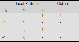
To realize a two input AND function we need a net with two input units and one output unit. A bias is also needed. Hence the structure of the required neural net should be as shown in Fig. 6.35. Moreover, the input and output signals must be in bipolar form, rather than the binary form, so that the net may be trained properly. The advantage of bipolar signals over binary signals is discussed in greater detail in Chap. 7. Considering the truth table of AND operation, and the fact that the bias is permanently set to 1, we get the training set depicted in Table 6.7.
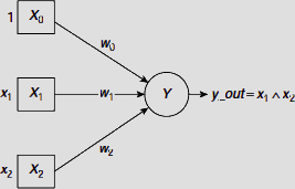
Fig. 6.35. Structure of a neural net to realize the AND function
Table 6.7 Training set for AND function
During the training process, all weights are initialized to 0. Therefore initially
At each training instance, the weights are changed according to the formula
where Δwi, the increment in wi, is computed as Δwi = xi.× t. After initialization, the progress of the learning process by the network is shown in Table 6.8.
Table 6.8. Hebbian learning of AND function
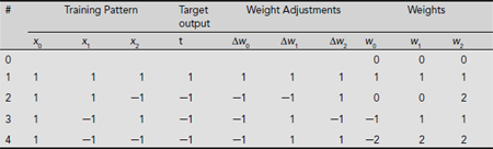
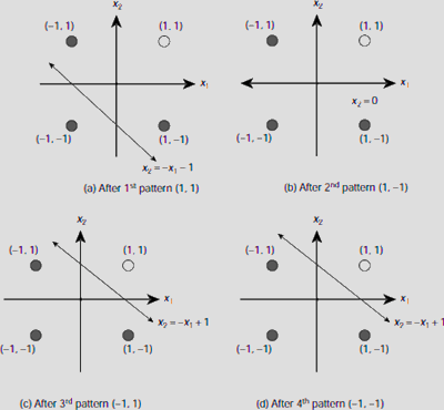
Fig. 6.36. Hebbian training to learn AND function
Hence, on completion of one epoch of training, the weight vector is W = [w0, w1, w2] = [–2, 2, 2]. The progress in learning by the net can be visualized by observing the orientation of the decision line after each training instance. Putting the values of the interconnection weights in the equation
we get
(i) |
x2 = −x1 – 1, |
after the 1st training instance, |
(ii) |
x2 = 0, |
after the 2nd training instance, |
(iii) |
x2 = −x1 + 1, |
after the 3rd training instance, and finally, |
(iv) |
x2 = −x1 + 1, |
after the 4th training instance. |
This progress in the learning process is depicted in Fig. 6.36(a)-(d). We see that after training with the first pattern [x0, x1, x2] = [1, 1, 1], the ANN learns to classify two patterns (–1, –1) and (1, 1) successfully. But it fails to classify correctly the other two patterns (–1, 1) and (1, –1). After learning with the second pattern (1, –1) the situation is better. Only (–1, 1) is still misclassified. This is corrected after training with the third pattern (–1, 1). Now all the –1 producing patterns are, i.e., (1, –1), (–1, 1) and (–1, –1) are in the same class and the remaining pattern (1, 1) constitutes the other class.
(b) Perceptron Learning Rule
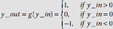
Let us consider a simple ANN consisting of a single perceptron Y with m+1 input units X0, …, Xm as shown in Fig. 6.17(b). The corresponding weights of the interconnections are w0, …, wm. The bias is introduced as the weight w0 connected to the input X0 whose activation is fixed at 1. For the output unit, it is convenient to use the bipolar activation function :
Now, let X = (x0, …, xm) be a training vector for which the output of the perceptron is expected to be t, where t = 1, 0, or –1. The current combination of the weights is given by the weight vector W = (w0, …, wm). If the perceptron produces the desired output, then the weights w0, …, wm need not be changed and they are to be kept unaltered. If, however, the perceptron misclassifies X negatively (meaning, it erroneously produces –1 instead of the desired output +1) then the weights should be appropriately increased. Conversely, the weights are to be decreased in case the perceptron misclassifies X positively (i.e., it erroneously produces +1 instead of the desired output –1). The learning strategy of the perceptron is summarized in Table 6.9.
Hence the perceptron learning rule is informally stated as
IF the output is erroneous THEN adjust the interconnection weights
ELSE leave the interconnection weights unchanged.
In more precise terms,
IF y_out ≠ t THEN
FOR i = 0 TO m DO wi(new) = wi(old) + η × t × xi
ELSE
FOR i = 0 TO m DO wi(new) = wi(old).
Table 6.9. Perceptron learning rules
# | Condition | Action |
|---|---|---|
1 | The perceptron classifies the input pattern correctly (y_out = t) | No change in the current set of weights w0, w1, …, wm. |
2 |
The perceptron misclassifies the input pattern negatively (y_out = –1, but t = +1) | Increase each wi by Δwi, where Δwi is proportional to xi, for all i = 0, 1, …, m. |
3 |
The perceptron misclassifies the input pattern positively (y_out = +1, but t = –1) |
Decrease each wi by Δwi, where Δwi is proportional to xi, for all i = 0, 1, …, m. |
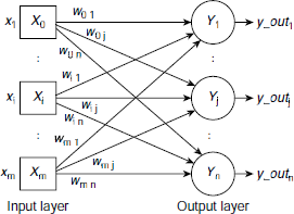
Fig. 6.37. Structure of an ANN with several perceptrons
Thus the perceptron learning rule can be formulated as
Here η is a constant known as the learning rate. It should be noticed that when a training vector is correctly classified then y_out = t, and the weight adjustment Δwi= 0. When y_out = –1 but t = +1, i.e., the pattern is misclassified negatively, then t – y_out = +2 so that Δwi is incremental and is proportional to xi. If, however, the input pattern is misclassified positively, the adjustment is decremental, and obviously, proportional to xi. Using matrix notation, the perceptron learning rule may now be written as
where, ΔW and X are the vectors corresponding to the interconnection weights and the inputs.
Equation 6.45 can be easily extended to a network of several perceptrons at the output layer. Such architecture is shown in Fig. 6.37. The net inputs to the perceptrons are
or,
For such an ANN, the adjustment Δwij of the weight wij is given by
Let us assume the following matrix notations :
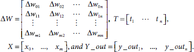
Then the expression of the perceptron learning rule for the architecture shown in Fig. 6.34 becomes
Example 6.7 (Learning the logical AND function by a perceptron)
Let us train a perceptron to realize the logical AND function. The training patterns and the corresponding target outputs for AND operation where the input and outputs are in bipolar form are given in Table 6.7. The structure of the perceptron is same as shown in Fig. 6.35. Activation function for the output unit is :
The successive steps of computation with the first training pair are given below.
- Initialize weights : w0 = w1 = w2 = 0, and the learning rate η = 1.
- For the training pair s : t = (1, 1, 1) : (1), compute the net input y_in and the activation y_out:
y_in = w0 × x0 + w1 × x1 + w2 × x2= 0 × 1 + 0 × 1 + 0 × 1= 0∴ y_out = 0.
- Apply the perceptron learning rule to find the weight adjustments. The rule is :
If y_out = t, then the weights are not changed, otherwise change the weights according to the formula wi (new) = wi (old) + Δwi where Δwi = ηt xi. In the present case, y_out =0, and t = 1, and y_out ≠ t. Therefore the weights are to be adjusted.
Similarly,
And,
Putting these values of the weights in the formula
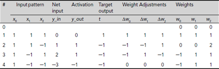
we get the separating line as x2 = −x1 − 1, which classifies the patterns (1, 1) and (–1, –1) correctly but misclassifies the patterns (–1, 1) and (1, –1) (Fig. 6.36(a)). A trace of the remaining steps of the first epoch of training (an epoch of training consists of successive application of each and every training pair of the training set for once) are noted in Table 6.10.
Hence, the set of weights obtained at the end of the first epoch of training is (–1, 1, 1) which represents to the decision line
It can be easily verified that this line (and the corresponding set of weights) successfully realizes the AND function for all possible input combinations. Hence, there is no need of further training.
Table 6.10. Perceptron learning of AND function
(c) Delta / LMS (Least Mean Square), or, Widrow-Hoff Rule
Least Mean Square (LMS), also referred to as the Delta, or Widrow-Hoff Rule, is another widely used learning rule in ANN literature. Here the weight adjustment is computed as
where the symbols have their usual meanings. In LMS learning, the identity function is used as the activation function during the training phase. The learning rule minimizes mean squared error between the activation and the target value. The output of LMS learning is in binary form. Example 6.8 illustrates LMS learning of the AND function.
The training patterns and the corresponding target outputs for AND operation where the input and outputs are in bipolar form are given in Table 6.7. The structure of the perceptron is same as shown in Fig. 6.35. The successive steps of computation for the first epoch are given below.
- Initialize weights : w0 = w1 = w2 = .3, and the learning rate η = .2 (These values are randomly chosen)
- For the training pair s : t = (1, 1, 1) : (1), compute the net input y_in as
y_in = w0 × x0 + w1 × x1 + w2 × x2= .3 × 1 + .3 × 1 + .3 × 1= .9
- Apply the LMS learning rule to find the weight adjustments. The rule is, wi (new) = wi (old) + Δwi, where Δwi = η(t − y_in) xi. Hence
wi (new) = wi (old) + η(t – y_in) xi,
In the present case, y_in = .9, and t = 1. Therefore
w0 (new) = w0 (old) + Δw0= w0 (old) + η(t – y_in) x0= .3 + .2 × (1 − .9) × 1= .3 + .02= .32Similarly,
w1 (new) = w2 (new) = .32Second iteration is to be carried out with the training pair s : t = (1, 1, −1) : (−1). The net input y_in is now
y_in = w0 × x0 + w1 × x1 + w2 × x2= .32 × 1 + .32 × 1 + .32 × (−1)= .32The new weights are computed as follows :
w0 (new) = w0 (old) + Δw0= w0 (old) + η(t – y_in) x0= .32 + .2 × (−1 − .32) × 1= .32 − .264= .056Similarly,
w1 (new) = .056However,
w2 (new) = .32 + .2 × (−1 − .32) × (−1)= .32 + .264= .584
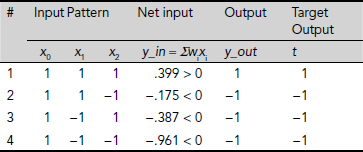
Hence, at the end of the second iteration, we get w0 = .056, w1 = .056, and w2 = .584. The details of the computation for the first epoch are recorded in Table 6.11. We see that the weights arrived at the end of the first epoch are w0 = –.281, w1 = .393, and w2 = .287. Table 6.12 shows that this set of weights is appropriate to realize the AND function. Hence there is no need to iterate further.
Table 6.11. LMS Learning of AND function
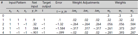
Table 6.12. Performance of the net after LMS learning
(d) Extended Delta Rule
The Extended Delta Rule removes the restriction of the output activation function being the identity function only. Any differentiable function can be used for this purpose. Here the weight adjustment is given by
where g(.) is the output activation function and g′(.) is its first derivative.
6.7.2 Unsupervised Learning
So far we have considered only supervised learning where the training patterns are provided with the target outputs. However, the target output may not be available during the learning phase. Typically, such a situation is posed by a pattern clustering problem, rather than a classification or association problem.
Let us, for instance, consider a set of points on a Cartesian plane as shown in Fig. 6.38 (a). The problem is to divide the given patterns into two clusters so that when the neural net is presented with one of these patterns, its output indicates the cluster to which the pattern belongs. Intuitively, the patterns those are close to each other should form a cluster. Of course we must have a suitable measure of closeness. Fig. 6.38(b) shows the situation after the neural net learns to form the clusters, so that it ‘knows’ the cluster to which each of the given pattern belongs.
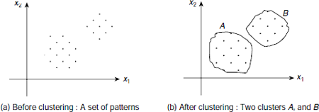
Fig. 6.38. Clustering a given set of patterns
Clustering is an instance of unsupervised learning because it is not assisted by any teacher, or, any target output. The network itself has to understand the patterns and put them into appropriate clusters. The only clue is the given number of clusters. Let us suppose that the network output layer has one unit for each cluster. In response to a given input pattern, exactly one among the output units has to fire. To ensure this, additional features need to be included in the network so that the network is compelled to make a decision as to which unit should fire due to certain input pattern. This is achieved through a mechanism called competition. The most commonly used competitive learning mechanism is the so called winner-takes-all learning. The basic principle of winner-take-it-all is discussed below.
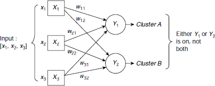
Fig. 6.39. A 3 input 2 output clustering network
Winner-takes-all Let us consider a simple ANN consisting of three input units and two output units as shown in Fig. 6.39. As each input unit of a clustering network corresponds to a component of the input vector, this network accepts input vectors of the form [x1, x2, x3]. Each output unit of a clustering network represents a cluster. Therefore the present network will divide the set of input patterns into two clusters. The weight vector for an output unit in a clustering network is known as the exemplar or code-book vector for the vectors of the cluster represented by the corresponding output unit. Hence, for the net in Fig. 6.39, the weight vector [w11, w21, w31] is an exemplar (or code-book vector) for the patterns of cluster A. Similarly, [w12, w22, w32] is the exemplar for the patterns of cluster B.
In the winner-takes-all strategy, the network finds the output unit that matches best for the current input vector and makes it the winner. The weight vector for the winner is then updated according to the learning algorithm. One way of deciding the winner is to employ the square of the Euclidean distance between the input vector and the exemplar. The unit that has the smallest Euclidean distance between its weight vector and the input vector is chosen as the winner. The algorithmic steps for an m-input n-output clustering network are given below:
- For each output unit Yj, j = 1 to n, compute the squared Euclidean distance as
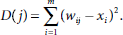
- Let YJ be the output unit with the smallest squared Euclidean distance D(J).
- For all output units within a specified neighbourhood of YJ, update the weights as follows :
wij (new) = wij (old) + η × [xi – wij (old)]
The concepts of neighbourhood, and winner-takes-all, in general, will be discussed in greater detail in the chapter on competitive neural nets. Example 6.9 illustrates the winner-takes-all strategy more explicitly.
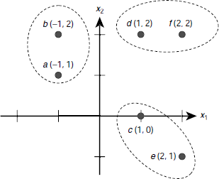
Fig. 6.40. A clustering problem showing the expected clusters
Example 6.9 (Competitive learning through Winner-takes-all strategy)
Let us consider a set of six patterns S = {a (–1, 1), b (–1, 2), c (1, 0), d (1, 2), e (2, –1), f(2, 2)}. The positions of these points on a two dimensional Eucledian plane are shown in Fig. 6.40. Intuitively, the six points form three clusters {a, b}, {d, f}, and {c, e}. Given the number of clusters to be formed as 3, how should a neural net learn the clusters by applying the winner-takes-all as its learning strategy? Let us see.
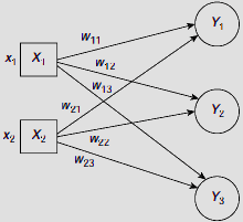
Fig. 6.41. A 2 input 3 output ANN to solve the clustering problem of Example 6.9
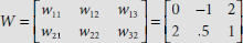
The input patterns are of the form (x1, x2) and the whole data set is to be partitioned into three clusters. So the target ANN should have two input units and three output units (Fig. 6.41). Let the initial distribution of (randomly chosen) weights be
This means that the exemplars, or code vectors, are initially C1 = (w11, w21) = (0, 2), C2 = (w12, w22) = (–1, 0), and C3 = (w13, w23) = (2, 1). The positions of the code vectors as well as the patterns to be clustered are shown in Fig. 6.42.
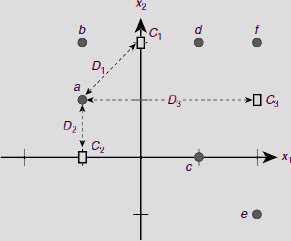
Fig. 6.42. Initial positions of the code vectors
Clusters are formed on the basis of the distances between a pattern and a code vector. For example, to determine the cluster for the pattern a (–1, 1) we need to compute the Euclidean distance between the point a and each code vector C1, C2, C3. The pattern is then clustered with nearest among the three code vectors. Let D1, D2, D3 be the squares of the Euclidean distances between a pattern and C1, C2, C3 respectively. For a (–1, 1) the computations of D1, D2, D3 are as follows.
Since D2 is the minimum among these the pattern a (–1, 1) the corresponding exemplar C2 is declared the winner and the pattern is clustered around the code vector C2. Similar computations for the pattern b (–1, 2) are given below.
In this case D1 is the minimum making C1 the winner. Table 6.13 summarizes the initial clustering process yielding the clusters C1 = {b, d}, C2 = {a} and C3 = {c, e, f} (Fig. 6.43). The minimum distance is indicated by a pair of parentheses.
Table 6.13. Initial cluster formation
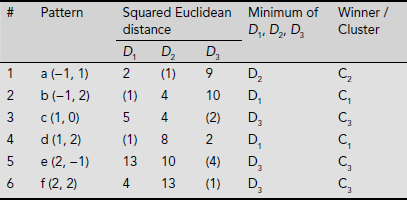
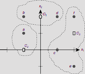
Fig. 6.43. Initial clusters
The initial clustering depicted in Fig. 6.43 is neither perfect, nor final. This will change as the learning proceeds through a number of epochs. This is explained below.
We take the value of the learning rate η =0.5 and follow the steps of winner-takes-all strategy to modify the positions of the exemplars so that they represent the respective clusters better. The process is described below.
(a) 1st Epoch
- Find the winner for the pattern a (–1, 1) and adjust the corresponding code-vector
D1 = (w11 – x1)2 + (w21 – x2)2 = (0 + 1)2 + (2 – 1)2 = 2D2 = (w12 – x1)2 + (w22 – x2)2 = (−1 + 1)2 + (0 – 1)2 = 1D3 = (w13 – x1)2 + (w23 – x2)2 = (2 + 1)2 + (1 – 1)2 = 9
Since D2 is the minimum among these, the winner is C2. Hence the weights w12 and w22 are to be changed. The new weights are obtained as
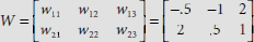
w12 (new) = w12 (old) + η (x1 − w12 (old)) = −1 + .5 × (−1 + 1) = −1w22 (new) = w22 (old) + η (x2 – w22 (old)) = 0 + .5 × (1 − 0) = .5The new code vector C2 is (–1, .5). It is closer to the training vector a (–1, 1) than the old code vector (–1, 0) (Fig. 6.44(b)). The weight matrix now changes to
- Find the winner for the pattern b (–1, 2) and adjust the corresponding code-vector
D1 = (w11 – x1)2 + (w21 – x2)2 = (0 + 1)2 + (2 – 2)2 = 1D2 = (w12 – x1)2 + (w22 – x2)2 = (−1 + 1)2 + (.5 – 2)2 = 2.25D3 = (w13 – x1)2 + (w23 – x2)2 = (2 + 1)2 + (1 – 2)2 = 10
Since D1 is the minimum among these, the winner is C1. Hence the weights w11 and w21 are to be changed. The new weights are obtained as
w11 (new) = w11 (old) + η (x1 − w11 (old)) = 0 + .5 × (−1 − 0) = −.5w21 (new) = w21 (old) + η (x2 – w21 (old)) = 2 + .5 × (2 − 2) = 2The new code vector C1 is (–.5, 2). It is closer to the training vector b (–1, 2) than the old code vector (0, 2) (Fig. 6.44(c)). The new weight matrix is
The successive iterations of the 1st epoch with the rest of the training vector are carried out in a similar fashion and are summarized in Table 6.14. The corresponding changes in the positions of the code vectors are depicted in Fig. 6.44(b)-(g).
Table 6.14. Clustering process during the 1st epoch
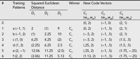
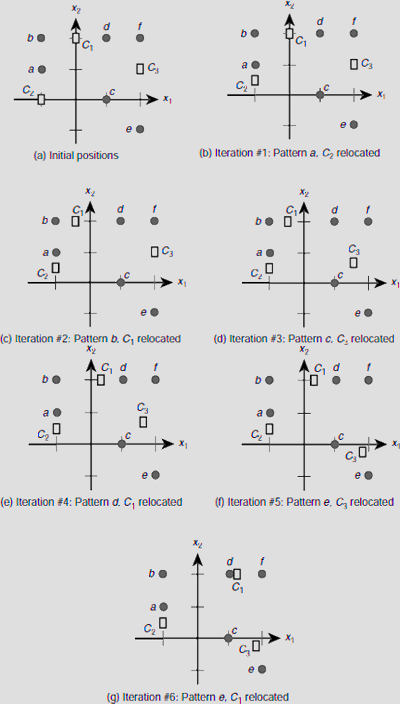
Fig. 6.44. Successive positions of the code vectors during the 1st epoch of the clustering process
Table 6.15. Clusters after the 1st epoch
# |
Training Vector |
Cluster |
|---|---|---|
1 |
a (−1, 1) |
C2 |
2 |
b (−1, 2) |
C2 |
3 |
c (1, 0) |
C3 |
4 |
d (1, 2) |
C1 |
5 |
e (2, −1) |
C3 |
6 |
f (2, 2) |
C1 |
Clusters formed
C1 |
: |
{d, f} |
C2 |
: |
{a, b} |
C3 |
: |
{c, e} |
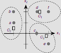
Fig. 6.45. Clusters formed after the 1st epoch
Therefore, the weight matrix at the end of the first epoch is obtained as
The corresponding clusters can be easily found by computing the distance of each training vector from the three code vectors and attaching it to the cluster represented by the nearest code vector. Table 6.15 summarizes these results and Fig. 6.45 shows the clusters formed at the end of the 1st epoch. It is obvious from Fig. 6.45 that the clusters formed conform to our intuitive expectation. However, this should be further consolidated by a second epoch of training.
(b) 2nd Epoch
Table 6.16. Clustering process during the 2nd epoch
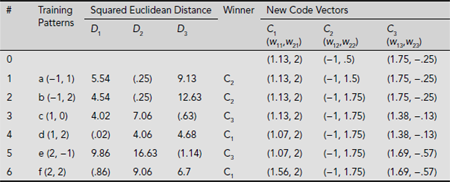
The summary of the second epoch of training is given in Table 6.16. Table 6.17 shows the clusters formed at the end of this epoch and Fig. 6.46 depicts the location of the code vectors as well as the corresponding clusters. It should be noted that though the clusters has not changed from the first epoch, the positions of the exemplars has changed. In fact, these have moved towards the ‘centre’ of the respective clusters. This is expected, because the exemplar is the representative of a cluster.
Table 6.17. Clusters after the 2nd epoch
# |
Training Vector |
Cluster |
|---|---|---|
1 |
a (−1, 1) |
C2 |
2 |
b (−1, 2) |
C2 |
3 |
c (1, 0) |
C3 |
4 |
d (1, 2) |
C1 |
5 |
e (2, −1) |
C3 |
6 |
f (2, 2) |
C1 |
Clusters formed
C1 |
: |
{d, f} |
C2 |
: |
{a, b} |
C3 |
: |
{c, e} |
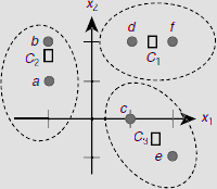
Fig. 6.46. Clusters formed after the 2nd epoch
CHAPTER SUMMARY
Certain fundamental concepts of artificial neural networks have been presented in this chapter. The main points of the foregoing text are summerized below.
- ANNs are inspired by the biological brain that processes data in terms of patterns rather than sequential fetch and execute cycle of instruction execution by a classical Von Neuman digital computer.
- Information is stored in brain as strengths of the synaptic gaps between the neurons. Similarly, knowledge is stored in an ANN as weights of interconnection between neural processing units. Thus both the brain and the ANN stores information in a distributed manner.
- ANNs are suitable for problem related to pattern classification and pattern association.
- The earliest artificial neural model was proposed by McCulloch and Pitts in 1943.
- The perceptron model was proposed by Rosenblatt in 1962. It has the nice property of being able to learn to classify a linearly separable set of patterns.
- ANNs have various architectures, such as, single-layer feed forward, multy-layer feed forward, competitive networks, recurrent networks etc.
- Certain functions such as the identity function, the step function, the sigmoid function, the hyperbolic tangent function etc. are widely used as activation functions in an ANN.
- There are two kinds of learning methods for an ANN, supervised and unsupervised. Learning takes place with the help of a set of training patterns. Under supervised learning each training pattern is accompanied by its target output. These target outputs are not available during unsupervised learning.
- The formulae for interconnection weight adjustment Δwi for different learning rules are shown in Table 6.18.
Table 6.18. Summary of ANN learning rules
#Learning RuleFormula for Δwi1
Hebb
Δwi = xi × t
2
Perceptron
Δwi = η × (t – y_out) × xi,
3
Delta/LMS/Widrow-Hoff
Δwi = η × (t – y_in) × xi
4
Extended delta
Δwij = η × (tj – y_outj) × x1 × g′(y_inj)
5
Winner-takes-all
Δwij = η ×[xi − wij (old)]
- The weight vector associated with an output of a clustering ANN is called the exemplar or the code-book vector. It represents the cluster corresponding to the output unit of the clustering ANN.
SOLVED PROBLEMS
Problem 6.1 Write MATLAB Code to realize the logical AND function with a neural net that learns the desired function through Hebb learning.
Solution 6.1 The MATLAB code and the output are given below as Fig. 6.47 and Fig. 6.48.
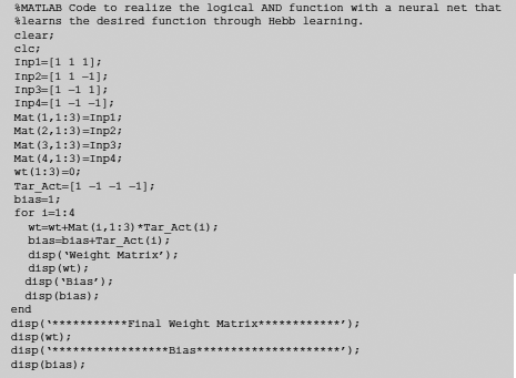
Fig. 6.47. MATLAB code for Hebb learning of AND function by an ANN
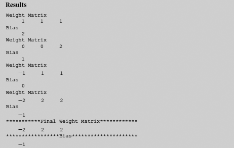
Fig. 6.48. MATLAB results for Hebb learning of AND function
Problem 6.2 Write MATLAB Code to realize the logical AND function with a neural net that learns the desired function through Perceptron learning.
Solution 6.2 The MATLAB code for the purpose is given below in Fig. 6.49. Fig. 6.50 presents the corresponding screenshot.
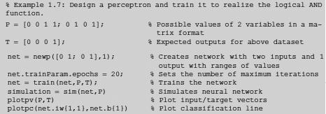
Fig. 6.49. MATLAB code for perceptron learning of AND function
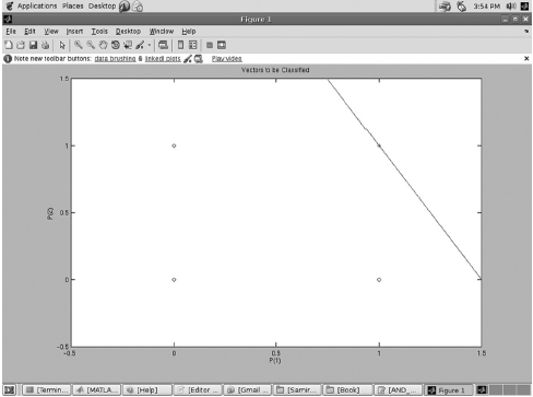
Fig. 6.50. MATLAB output for perceptron implementing AND function
Problem 6.3 Write MATLAB Code to realize the logical AND function with a neural net that learns the desired function through LMS learning.
Solution 6.3 The MATLAB code for the purpose is given in Fig. 6.51. Fig. 6.52 shows the results and screenshot is shown in Fig. 6.53.
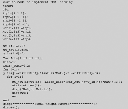
Fig. 6.51. MATLAB code for LMS learning of AND function by an ANN
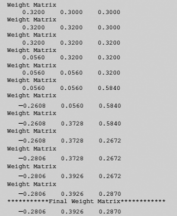
Fig. 6.52. MATLAB results for LMS learning of AND function

Fig. 6.53. MATLAB screen showing results of LMS learning of AND function
Problem 6.4 Write MATLAB Code to implement the Winner-takes-all strategy of pattern clustering.
Solution 6.4 The MATLAB code is shown in Fig. 6.54. The data set is taken from Example 6.9.
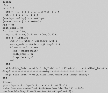
Fig. 6.54. MATLAB code for clustering through winner-takes-all
TEST YOUR KNOWLEDGE
6.1 Which of the following parts of a biological neuron is modeled by the weighted interconnections between the input units and the output unit of an artificial neural model?
- Dendrite
- Axon
- Soma
- Synapse
6.2 The effect of the synaptic gap in a biological neuron is modeled in artificial neuron model as
- The weights of the interconnections
- The activation function
- The net input to the processing element
- None of the above
6.3 In an artificial neural model, the activation function of the input unit is
- The step function
- The identity function
- The sigmoid function
- None of the above
6.4 Which of the following is not true about Perceptrons ?
- It can classify linearly separable patterns
- It does not have any hidden layer
- It has only one output unit
- None of the above
6.5 Recognition of hand written characters is an act of
- Pattern classification
- Pattern association
- Both (a) and (b)
- None the above
6.6 Identification of an object, e.g., a chair, a tree, or a human being, from the visual image of our surroundings, is an act of
- Pattern classification
- Pattern association
- Both (a) and (b)
- None the above
6.7 The interconnections of a Hopfield network are
- Unidirectional
- Bidirectional
- Both (a) and (b)
- None the above
6.8 The interconnections of a perception are
- Unidirectional
- Bidirectional
- Both (a) and (b)
- None the above
6.9 Parallel relaxation is a process related to the functionality of
- Perceptrons
- McCulloch-Pitts neurons
- Hopfield networks
- None the above
6.10 In which of the following ANN models the inhibition is absolute, i.e., a single inhibitive input can prevent the output to fire, irrespective of the number of excitatory inputs?
6.11 Which of the following is not true about McCulloch-Pitts neurons?
- The interconnections are unidirectional
- All excitatory interconnections have the same weight
- All inhibitory interconnections have the same weight
- The activation is bipolar
6.12 Which of the following operations can be realized by a network of McCulloch-Pitts neurons, but not a network of perceptions?
- Logical AND
- Logical OR
- Logical XOR
- None the above
6.13 Which of the following kinds of classification problems can be solved by a perception?
- Linearly separable
- Non-linearly separable
- Both (a) and (b)
- None the above
6.14 Which of the following entities is guaranteed by the Perceptron Convergence Theorem to converge during the learning process?
- The output activation
- The interconnection weights
- Both (a) and (b)
- None the above
6.15 The XOR function cannot be realized by a Perceptron because the input patterns are
- Not bipolar
- Not linearly separable
- Discrete
- None the above
6.16 The XOR function can be realized by
- A Perceptron
- A network of Perceptrons
- A Hopfield network
- None the above
6.17 Which of the following ANN architectures contains bidirectional interconnections?
- Single-layered feed forward
- Multi-layered feed forward
- Competitive networks
- None the above
6.18 Which of the following activation functions is not differentiable?
- Identity function
- Heaviside function
- Sigmoid function
- None the above
6.19 Which of the following ANN learning algorithms is not a supervised learning?
- Perceptron learning
- Widrow-Hof learning
- Winner-takes-all
- None the above
6.20 During learning, if a Perceptron misclassifies a training data negatively, i.e., erroneously yields an output –1 instead of +1, the interconnection weights are to be
- Increased
- Decreased
- Kept unaltered
- None the above
6.21 During learning, if a Perceptron misclassifies a training data positively, i.e., erroneously yields an output +1 instead of –1, the interconnection weights are
- Increased
- Decreased
- Kept unaltered
- None the above
6.22 Which of the following learning rules does not guarantee to learn a classification instance even if the classes are linearly separable ?
- Perceptron learning rule
- Hebb rule
- Both (a) and (b)
- None of the above
6.23 Which of the following is a competitive learning method?
- Winner-takes-all
- Least-Mean-square
- Extended delta
- None the above
6.24 The weight vector attached to an output unit of a clustering network is known as
- an exemplar
- a code vector
- Both (a) and (b)
- None of the above
6.25 Which of the following ANN learning methods use Euclidean distance between the weight vector and the input vector to compute the output ?
- Perceptron learning
- Widrow-Hoff learning
- Winner-takes-all learning
- None of the above
Answers
6.1 (d) |
6.2 (a) |
6.3 (b) |
6.4 (d) |
6.5 (b) |
6.6 (a) |
6.7 (b) |
6.8 (a) |
6.9 (c) |
6.10 (c) |
6.11 (d) |
6.12 (d) |
6.13 (a) |
6.14 (b) |
6.15 (b) |
6.16 (b) |
6.17 (c) |
6.18 (b) |
6.19 (c) |
6.20 (a) |
6.21 (b) |
6.22 (b) |
6.23 (a) |
6.24 (c) |
6.25 (c) |
EXERCISES
6.1 There are two ways to interpret the role of the brain while considering the human body as a computational agent. One of them is to view the entire brain as a single unit that acts as the CPU for the whole body. The other is to consider the brain as a huge network of billions of processing units called neurons. Compare and contrast between these two views from computational perspective.
6.2 The majority function outputs a 0 if there are more 0s in the inputs than 1s, and outputs a 1 if there are more 1s in the inputs than 0s. In short, it returns the majority input to the output. The truth table for a 3 input majority function is given as Table 6.19. Design a McCulloch-Pitts neural net to realize the 3-input majority function.
Table 6.19. Three input majority function
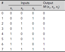
6.3 Consider the sets of points A and B shown in Fig. 6.54 where A = {a (–1, 1), b (–1, 0), c (–1, –1), e (0, 0), f (0, –1)} and B = {d (0, 2), g (1, 2), h (1, 1), i (2, 2), j (2, 1)}. Propose two different Perceptrons to classify these sets of patterns by observation, analysis, and understanding only (and not by learning).
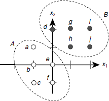
Fig. 6.54. A classification problem instance
6.4 Consider the 3-input majority function cited in Exercise No. 6.2. Fig. 6.55 shows the positions of the input patterns in a 3-dimensional space, classified on the basis of the corresponding output values. Are these patterns linearly separable? If so, propose a perceptron to realize this function.
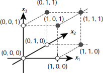
Fig. 6.55. Three input majority function
6.5 Draw the structure of a 3-3-2 multi-layered feed forward neural net. Also, present the matrix algebraic expression for the net inputs and the outputs of each layer.
6.6 Train a neural net through the Hebb rule to realize the logical OR function.
6.7 Realize the 3-input majority function through the Perceptron learning rule.
6. 8 Train a neural net through the LMS rule to realize the logical OR function.
6.9 Let S be a set of six points on an Euclidean plane where S = {a (0, –1), b (0, –2), c (1, 2), d (1, 1), e(1, –1), f (2, 1)} (Fig. 6.56). Taking the initial code vectors as C1 = (0, 0), and C2 = (–1, –2) find i) the initial clusters, and ii) final cluster with the help of winner-takes-all strategy.

Fig. 6.56. A clustering problem with initial code vectors
BIBLIOGRAPHY AND HISTORICAL NOTES
Research in the area of ANNs started in early 40s, when neuro-physiologist, Warren McCulloch and mathematician Walter Pitts proposed their celebrated McCulloch-Pitts Theory of Formal Neural Networks. They even designed and developed a primitive ANN using simple electric circuits. The theories of McCulloch and Pitts on the nature and functionalities of neurons were further supported by Donald Hebb in his 1949 book ‘The organization of behaviour’. In 1954 Marvin Minsky wrote his Ph.D. thesis entitled ‘Theory of Neural-Analog Reinforcement Systems and its Application to the Brain-Model Problem’, which is widely acclaimed as an important early research into neural networks. Then in 1958 Frank Rosenblatt, a neuro-biologist at Cornell University, proposed the Perceptron, the first ‘practical’ ANN. However, Marvin Minsky and Seymour Papert proved in their book of 1969 entitled ‘Perceptrons’ that the capabilities of perceptrons are very limited. As a consequence, enthusiasm declined over the subsequent few years. The first neural networks that could be applied to real problems, ADALINE (ADAptive LINear Elements) and MADALINE (Multiple ADAptive LINear Elements), were developed by Bernard Wildrow and Marcian Hoff of Stanford University between 1959 and 1960. In 1982 John Hopfield of Caltech presented some new ideas in neural networks that eventually came to be known as Hopfield networks. A new era in neural networks started in 1986 when Rumelhart, Hinton and Williams proposed the back-propagation algorithm to overcome the limitations of perceptron. Many more developments took place in the last few decades in the field of ANNs. A few seminal works in this area are referred below.
Anderson, J. A. and Rosenfield, E., (eds). (1988). Neurocomputing: Foundations of research. Cambridge, MA, MIT Press.
Angeniol, B., Vaubois, G., and Le Texier, J.-Y. (1988). Self-organizing feature maps and the traveling salesman problem. Neural Networks, 1(4), pp. 289–293.
Block, H. D. (1962). The perceptron: A model for brain functioning. Reviews for modern physics. Vol. 34, pp. 123–135.
Cohen, M. A. and Grossberg, S. (1983). Absolute stability of global pattern formation and parallel memory storage by competitive neural networks. IEEE transactions on Systems, Man and Cybernetics, SMC-13, pp. 815–826.
Hopfield, J. J. (1982). Neural networks and physical systems with emergent collective computational properties. Proc. of the National Academy of Sciences of the USA, 79, pp. 2554–2588.
Hopfield, J. J. and Tank, D. W. (1985). Neural computation of decisions in optimization problems. Biological cybernetics, 52(3), pp. 141–152.
Hopfield, J. J. and Tank, D.W. (1986). Computing with neural circuits. Science, 233, pp. 625–633.
Grossberg, S. (1973). Contour enhancement, short-term memory, and constancies in reverberating neural networks. Studies in Applied Mathematics, 52.
Grossberg, S. (1982). Studies of mind and brain. Boston, Reidel.
Hebb, D. O. (1949). The organization of behaviour. New York, John Wiley and Sons.
Kohonen, T. (1982). Self-organized formation of topologically correct feature maps. Biological cybernetics, 43, pp. 59–69.
McCulloch, W. and Pitts, W. (1943). A logical calculus of the ideas immanent in nervous activity. Bulletin of Mathematical Biophysics, 7, pp. 115–133.
Minsky, M. and Papert, S. (1969). Perceptrons. MIT Press.
Rosenblatt, F. (1959). Two theorems of statistical separability in the perceptron. Mechanization of thought process: proceedings of the symposium at National Physical Laboratory, London, pp. 421–456.
Rosenblatt, F. (1962). Principles of Neurodynamics. Spartan Books.
Rumelhart, D. E., Hinton, G. E. and Williams, R. J. (1986). Learning representations by back-propagating errors. Nature, 323, pp. 533–536.
Tank, D. W., and Hopfield, J. J. (1987). Collective computation in neuronlike circuits. Scientific American, 257, pp. 104–114.
Von Neumann, J. (1958). The computer and the brain. New Haven : Yale University Press.
Widrow, B. and Hoff, M. E. (1960). Adaptive switching circuits. IRE WESCON convention record, part 4, pp. 96–104.