9
Competitive Neural Nets
Key Concepts
Adaptive resonance theory (ART), ART–1, ART–2, Clustering, Code vector, Competition, Exemplar, Inhibitory weight, Learning vector quantization (LVQ), MaxNet self-organizing map (SOM), Stability-plasticity dilemma, Topological neighbourhood, Vigilance parameter, Winner-takes-all
Chapter Outline
9.2 Kohonen’s Self-organizing Map (SOM)
9.3 Learning Vector Quantization
The last two chapters presented certain neural networks for pattern classification and pattern association. Artificial neural nets are inherently structured to suit such purposes. However, there are situations when the net is responded by more than one outputs even though it is known that only one of several neurons should respond. Therefore, such nets must be designed in a way so that it is forced to make a decision as to which unit would respond. This is achieved through a mechanism called competition and neural networks which employ competition are called competitive neural nets.
Winner-takes-all is a form of competition where only one among a group of competing neurons has a non-zero output at the end of computation. However, quite often the long iterative process of competition is replaced with a simple search for the neuron with the largest input, or some other criteria, to select as the winner.
There are various forms of learning by competitive nets. Maxnet, an elementary competitive net, does not require any training because its weights are fixed and pre-determined. Learning Vector Quantization (LVQ) nets avail training pairs to learn and therefore, the learning is supervised. However, an important type of competitive nets called the self-organizing map (SOM) which groups data into clusters employs unsupervised learning. A net employing unsupervised learning seeks to find patterns, or regularity, in the input data. Adaptive Resonance Theory (ART) nets are also clustering nets.
There are two methods to determine the closeness of a pattern vector to the weight vector. These are, Euclidean distance, and the dot product. The largest dot product corresponds to the smallest angle between the input and the weight vector if they are both of unit length.
The rest of this chapter presents brief discussions on four important competitive networks, viz., the Maxnet, Kohonen’s self-organizing maps, Learning Vector Quantization (LVQ) nets, and the Adaptive Resonance Theory (ART) nets.
9.1 THE MAXNET
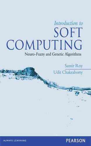
MAXNET is the simplest artificial neural net that works on the principle of competition. It is a fully connected network with symmetric interconnections and self-loops. The architecture of an m-unit MAXNET is shown in Fig. 9.1. It consists of m number of cluster units denoted as Y1,…, Ym. Each unit is directly connected to each other through a link. All the links have the same, fixed, inhibitory weight −δ. Each unit has a self-loop. The weight of a self-loop is 1. Each unit of a MAXNET represents a cluster. When the net is presented with an unknown pattern, the net iteratively modifies the activations of its units until all units except one attain zero activation. The remaining unit with positive activation is the winner.
Fig. 9.1. Architecture of an m-node MAXNET
9.1.1 Training a MAXNET
There is no need to train a MAXNET because all weights are fixed. While the self-loops have the weight 1, other interconnection paths have the same inhibitory weight −δ, where δ has to satisfy the condition ![]() , m being the number of units in the net.
, m being the number of units in the net.
9.1.2 Application of MAXNET
During application, the MAXNET is presented with an input vector x = [x1,…, xm] by initializing the activation of the ith unit Yi by xi, for all i = 1 to m. It then iteratively updates the activations of the cluster units using the activation function

Fig. 9.2. Algorithm MAXNET Clustering

Fig. 9.3. Flow chart for MAXNET Clustering
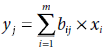
The net input to a cluster unit Yi is computed as
As the clustering process advances, more and more clustering units get deactivated (by attaining an activation of value 0) until all units except one are deactivated. The only one remaining positively activated unit is the winner. The procedure followed by MAXNET to identify the cluster to which a given pattern x = [x1,…, xm] belongs is described in Algorithm MAXNET–Clustering (Fig. 9.2). Fig. 9.3 presents a flowchart of the procedure. Example 9.1 illustrates the procedure followed by a MAXNET.
Example 9.1 (Clustering by MAXNET)
Let us consider the 4-unit MAXNET shown in Fig. 9.4. The inhibitory weight is taken as δ = 0.2 which satisfies the condition ![]() . The input pattern x = [x1, x2, x3, x4] = [0.5, 0.8, 0.3, 0.6] is to be clustered. The step-by-step execution of Algorithm MAXNET–Clustering is given below.
. The input pattern x = [x1, x2, x3, x4] = [0.5, 0.8, 0.3, 0.6] is to be clustered. The step-by-step execution of Algorithm MAXNET–Clustering is given below.

Fig. 9.4. A 4-unit MAXNET
Step 0. |
Initialize the net inputs to the cluster units. |
|
y_in1 = 0.5, y_in2 = 0.8, y_in3 = 0.3, y_in4 = 0.6
|
Iteration #1 |
|
Step 1. |
Compute the activation of each cluster unit. |
|
y_out1 = 0.5, y_out2 = 0.8, y_out3 = 0.3, y_out4 = 0.6. |
Step 2. |
Test for stopping condition. If all units except one have 0 activation Then return the unit with non-zero activation as the winner. Stop. |
|
There are four units with non-zero activations. Therefore the stopping criterion (that all units except one have zero activations) is not satisfied. Hence, continue to Step 3. |
Step 3. |
Update the net input to each cluster unit. |
|
= 0.5 − 0.2 × 1.7 = 0.5 − 0.34 = 0.16
|
|
|
|
y_in2 = 0.8 − 0.2 × (0.5 + 0.3 + 0.6) = 0.8 − 0.28 = 0.52 y_in3 = 0.3 − 0.2 × (0.5 + 0.8 + 0.6) = 0.3 − 0.38 = − 0.08 y_in4 = 0.6 − 0.2 × (0.5 + 0.8 + 0.3) = 0.6 − 0.32 = 0.28 |
Step 4. |
Go to Step 1. |
Iteration #2 |
|
Step 1. |
Compute the activation of each cluster unit. |
|
y_out1 = 0.16, y_out2 = 0.52, y_out3 = 0, y_out4 = 0.28 |
Step 2. |
Test for stopping condition. If all units except one have 0 activation Then return the unit with non-zero activation as the winner. Stop. |
|
There are three units with non-zero activations. Therefore the stopping criterion (that all units except one have zero activations) is not satisfied. Hence, continue to Step 3. |
Step 3. |
Update the net input to each cluster unit. |
|
= 0.16 − 0.2 × 0.8 = 0.16 − 0.16 = 0
|
Similarly, |
|
|
y_in2 = 0.432 |
|
y_in3 < 0 |
|
y_in4 = 0.144 |
Step 4. |
Go to Step 1. |
|
The calculations till the net comes to a halt is shown in Table 9.1. We see that the net successfully identifies the unit Y2 as having maximum input as all the other activations have been reduced to 0. Hence Y2 is the winner and the given input pattern is clustered to the cluster unit Y2. |
Table 9.1. Clustering by MAXNET

9.2 KOHONEN’s SELF-ORGANIZING MAP (SOM)
Kohonen’s self-organizing map (SOM) is a clustering neural net that works on the principle of winner-takes-all. The unique feature of Kohonen’s self-organizing map is the existence of a topological structure among the cluster units. It is assumed that the output (or, cluster) units are arranged in one- or two-dimensional arrays. Given a cluster unit Yj, its neighborhood of radius R is the set of all units within a distance of R around Yj. The idea is, patterns close to each other should be mapped to clusters with physical proximity.
A SOM that is used to cluster patterns of length m into n clusters should have m number of input units and n number of output, or cluster, units. The number of clusters is restricted by the number of output units n. Learning takes place with the help of a given set of patterns, and the given number of clusters into which the patterns are to be clustered. Initially, the clusters are unknown, i.e., the knowledge about the patterns that form a particular cluster, or the cluster to which a pattern belongs, is absent at the beginning. During the clustering process, the network organizes itself gradually so that patterns those are close to each other form a cluster. Hence, the learning here is unsupervised. The weight vector associated with a cluster unit acts as the exemplar for all patterns belonging to the cluster. During training, the cluster unit whose weight vector is closest to the given input pattern is the winner. The weight vectors of all cluster units in the neighborhood of the winner are updated.
Let s1, s2, …, sp be a set of p number of patterns of the form si = [xi1, xi2, …, xim], to be clustered into n clusters C1, C2, …, Cn. The subsequent neural net architecture and algorithm enables a Kohonen’s SOM to accomplish the clustering task stated above.
9.2.1 SOM Architecture
The architecture of a SOM is shown in Fig. 9.5. It consists of m input units X1, X2, …, Xm and n output units Y1, Y2, …, Yn. Each input unit Xi is connected to each output unit Yj through an edge with weight wij. Each output unit represents a cluster and these cluster units may be arranged in one, or two, dimensional arrays. The topological neighbourhood of a cluster unit in the Kohonen’s SOM is shown in Fig. 9.6. Fig. 9.6(a), (b), and (c) show 0, 1, 2 neighbourhood of a given cluster (represented as ⊗) in one and two dimensional array.

Fig. 9.5. Architecture of an m-input n-output SOM net
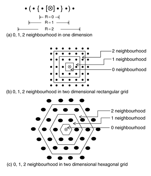
Fig. 9.6. Neighbourhood of a cluster unit in SOM
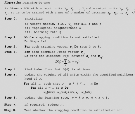
Fig. 9.7. Algorithm Learning-by-SOM
9.2.2 Learning by Kohonen’s SOM
Let {s1, s2, …, sp} be the set of training patterns where each si = [xi1, xi2, …, xim] is an m-dimensional vector. Learning by the SOM net starts with initializing the weights, the topological neighbourhood parameters, and the learning rate parameters. As mentioned earlier, SOM employs winner-takes-all strategy to organize itself into the desired clusters. The weight vector associated with a cluster unit represents an exemplar, or code-vector. Training takes place through a number of epochs. During an epoch of training, each training vector is compared with the exemplars and its distance from each exemplar is calculated. The cluster unit with least distance is the winner. The weight vector of the winner, along with the weight vectors of all units in its neighbourhood, is updated. After each epoch, the learning rate, and if necessary, the topological neighbourhood parameter, are updated. The learning algorithm is presented in Algorithm Learning-by-SOM (Fig. 9.7). The corresponding flowchart is given in Fig. 9.8.

Fig. 9.8. Flow chart for SOM learning
9.2.3 Application
During application, the input pattern is compared with the exemplar/code vector in terms of the distance between them. The cluster unit whose code vector is at a least distance from the input pattern is the winner. The input pattern belongs to the corresponding cluster.
The learning and application process of Kohonen’s self-organizing map are illustrated in Example 9.2 and Problem 9.1 in the Solved Problems section respectively.
Example 9.2 (Learning by Kohonen’s self-organizing map)
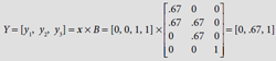
Suppose there are four patterns s1 = [1, 0, 0], s2 = [0, 0, 1], s3 = [1, 1, 0] and s4 = [0, 1, 1] to be clustered into two clusters. The target SOM, as shown in Fig. 9.9, consists of three input units and two output units.

Fig. 9.9. Target SOM network
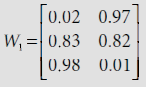
The exemplar, or code-vector, for the clusters C1 and C2, represented by the cluster units Y1 and Y2 respectively, are given by the 1st and the 2nd column of the weight matrix

Hence W*1 = [w11, w21, w31]T and W*2 = [w12, w22, w32]T are the code-vectors for the clusters C1 and C2 respectively. Now les us denote the input vectors as s1 = [1, 0, 0], s2 = [0, 0, 1], s3 = [1, 1, 0] and s4 = [0, 1, 1]. The successive steps of the learning process are described below.
Step 0. |
Initialize |
|
|
While stopping condition is not satisfied |
|
|
Do Steps 2–8. |
|
When the weight adjustment Δwij < 0.01 the net is assumed to have converged. Initially the stopping condition is obviously false. Hence we continue to Step 2. |
Step 2. |
For each training vector si Do Step 3 to 5. |
|
We start training with the first vector s1 = [1, 0, 0]. |
Step 3. |
For each exemplar /code vector w*j |
|
Do find the distance D(j) between si and w*j. |
|
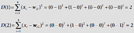
D (1) = distance between s1 and W*1
= (1 − 0.5)2 + (0 − 0.8)2 + (0 − 0.4)2
= 0.25 + 0.64 + 0.16
= 1.05
D (2) = distance between s1 and W*2
= (1 − 0.3)2 + (0 − 0.5)2 + (0 − 0.3)2
= 0.49 + 0.25 + 0.09
= 0.83
|
Step 4. |
Find index J so that D(J) is minimum. |
Since, D(2) < D(1), s1 is closer to C2, and Y2 is the winner. Therefore, the code vector W*2 is to be adjusted. |
|
Step 5. |
Update the weights of all units within the specified neighbourhood of J. |
For all J, such that J − R ≤ j ≤ J + R Do |
|
For all i = 1 to m Do |
|
|
wij (new) = wij (old) + η × [xi – wij (old)] |
|
Since R = 0, we need to adjust the weight vector of the winner only. |
|
|
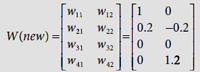
w12 (new) = w12 (old) + η × (x1 – w12 (old))
= 0.3 + 0.8 × (1 − 0.3)
= 0.3 + 0.8 × 0.7
= 0.86
w22 (new) = w22 (old) + η × (x2 – w22 (old))
= 0.5 + 0.8 × (0 − 0.5)
= 0.5 − 0.4
= 0.1
w32 (new) = w32 (old) + η × (x3 – w32 (old))
= 0.3 + 0.8 × (0 − 0.3)
= 0.3 − 0.24
= 0.06 | |
Hence, the weight matrix after training with the 1st input vector in the 1st epoch is |
|
 |
|
We now proceed to train the SOM with the second pattern. |
|
Step 2. |
|
After training with the first vector s1 = [1, 0, 0], we proceed with the second pattern s2 = [0, 0, 1]. |
|
Step 3. |
For each exemplar /code vector w*j |
Do find the distance D(j) between si and w*j. |
|
D (1) = distance between s2 and W*1
= (0 − 0.5)2 + (0 − 0.8)2 + (1 − 0.4)2
= 0.25 + 0.64 + 0.36
= 1.25
D (2) = distance between s2 and W*2
= (0 − 0.86)2 + (0 − 0.1)2 + (1 − 0.06)2
= 0.74 + 0.01 + 0.88
= 1.63
|
|
Step 4. |
Find index J so that D(J) is minimum. |
Since, D(1) < D(2), s2 is closer to C1, and Y1 is the winner. Therefore, the code vector W*1 is to be adjusted. |
|
Step 5. |
Update the weights of all units within the specified neighbourhood of J. |
For all J, such that J − R ≤ j ≤ J + R Do |
|
For all i = 1 to m Do |
|
|
wij (new) = wij (old) + η × [xi – wij (old)] |
|
Since R = 0, we need to adjust the weight vector of the winner only. |
|
|
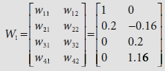
= 0.5 + 0.8 × (0 − 0.5)
= 0.5 − 0.8 × 0.5
= 0.1
w21 (new) = w21 (old) + η × (x2 – w21 (old))
= 0.8 + 0.8 × (0 − 0.8)
= 0.8 − 0.64
= 0.16
w31 (new) = w31 (old) + η × (x3 – w31 (old))
= 0.4 + 0.8 × (1 − 0.4)
= 0.4 + 0.48
= 0.88
|

Hence, the weight matrix W after training with the second vector in the first epoch is

In this way learning with the rest of the patterns s3 = [1, 1, 0] and s4 = [0, 1, 1] takes place by repeating Steps 3–5. Table 9.2 shows the outline of learning during the first epoch.
Table 9.2. Learning by the SOM during the first epoch

So, code-vector W*2 gets modified as a result of training with the patterns s1 and s3 while training with the patterns s2 and s4 results in adjustment of the code-vector W*1.
The weight matrix obtained after the first epoch is
On further computation, the weight matrix after the second epoch becomes

The training process converges after 19 epochs when the weight matrix becomes (approximately)

Fig. 9.10 shows the SOM obtained for the given clustering problem.
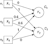
Fig. 9.10. Resultant net after training
9.3 LEARNING VECTOR QUANTIZATION (LVQ)
Another pattern clustering net based on the winner-takes-all strategy is Learning Vector Quantization (LVQ) nets. However, unlike Kohonen’s SOM, LVQ follows supervised learning, instead of unsupervised learning. The architecture of LVQ is essentially same as that of SOM except that the concept of topological neighbourhood is absent here. There are as many input units as the number of components in the input patterns and each output unit represents a known cluster. The details of LVQ learning are described below.
9.3.1 LVQ Learning
LVQ nets undergo a supervised learning process. The training set consists of a number of training vectors, each of which is designated with a known cluster. After initializing the weight matrix of the LVQ net, it undergoes training through a number of epochs. During each epoch, the weights are adjusted to accommodate the training vectors on the basis of their known clusters. The objective is to find the output unit that is closest to the input vector. In order to ensure this the algorithm finds the code vector w closest to the input vector s. If s and w map to the same cluster, then w is moved closer to s. Otherwise, w is moved away from x. Let t be the cluster for the training vector s, and Cj be the cluster represented by Yj, the jth output unit of the LVQ net. The procedure followed by LVQ learning is presented in Algorithm LVQ-Learning (Fig. 9.11). Fig. 9.12 presents the LVQ learning process in flowchart form.

Fig. 9.11. Algorithm LVQ-Learning

Fig. 9.12. Flow chart for LVQ Learning
9.3.2 Application
During application, the input pattern is compared with the exemplar/code vector in terms of the distance between them. The cluster unit whose code vector is at a least distance from the input pattern is the winner. The input pattern belongs to the corresponding cluster.
The learning and application process of LVQ nets are illustrated in Examples 9.3 and 9.4 respectively.
Five patterns and their corresponding designated clusters are given in Table 9.3. A neural net is to be obtained through Learning Vector Quantization (LVQ) method for the given set of vectors.
As there are 4 components in the training vectors and two clusters, the target net shall have 4 inputs and 2 cluster units. The exemplars, or code vectors, are initialized with the input vectors 1 and 4. The rest of the vectors, i.e., 2, 3, 5 are used for training. Fig. 9.13 shows the initial situation. Subsequent steps of the learning process are described below.
Table 9.3. Training set
# |
Training Vector s = [x1, x2, x3, x2] |
Cluster |
|---|---|---|
1 |
s1 = [1, 0, 0, 0] |
C1 |
2 |
s2 = [0, 1, 0, 0] |
C1 |
3 |
s3 = [1, 1, 0, 0] |
C1 |
4 |
s4 = [0, 0, 0, 1] |
C2 |
5 |
s5 = [0, 0, 1, 1] |
C2 |

Fig. 9.13. Initial configuration
Step 0. |
Initialize the weight matrix, and the learning rate. |
|
|
The weight matrix is initialized with the patterns s1 = [1, 0, 0, 0] and s4 = [0, 0, 0, 1]. The resultant weight vector is shown in Fig. 9.13. We fix the learning rate η = 0.2 and decrease it geometrically after each iteration by a factor of 0.5. |
Step 1. |
While stopping condition is not satisfied Do Step 2 to Step 7. |
We stop when the process converges, i.e., there is no perceptible change in the code vectors. Obviously, initially the stopping condition is false. |
|
Step 2. |
For each input training vector s Do Step 3 to Step 5. The first training vector is s2 = [0, 1, 0, 0] that maps to cluster C1. |
Step 3. |
Find the distance D(j) of s from each exemplar / code-vector W*j. |
|
 |
|
The distance of s2 = (0, 1, 0, 0) from the two code-vectors are calculated. |
|
 |
Step 4. |
Find the index J for which D(J) is minimum. |
|
As D(1) = D(2), we resolve the tie by arbitrarily selecting J = 2. |
Step 5. |
Update code-vector W*J. |
|
|
If t = = Cj Then /* bring Cj closer to s */
w*J (new) = w*J (old) + η ×[s – w*j (old)]
Else /* take Cj away from s */
w*J(new) = w*J(old) − η × [s – w*j(old)]
As per Table 9.4, t = C1 and therefore, t ≠ Cj here. Hence, the code vector W*2 should be moved away from the training pattern s2 = (0, 1, 0, 0) . Therefore,
w12(new) = w12(old) − η × [x1 – w12(old)]
= 0 − 0.2 × (0 − 0)
= 0.
w22(new) = w22(old) − η × [x2 – w22(old)]
= 0 − 0.2 × (1 − 0)
= −0.2
Similarly, w32(new) = 0, and w42(new) = 1.2. Hence the new weight matrix is, |
 |
|
|
We now go back to Step 2 to train the net with the next training pattern. |
Step 2. |
For each input training vector s Do Steps 3 to Step 5. The second training pattern is s3 = [1, 1, 0, 0] that maps to cluster C1. |
Step 3. |
Find the distance D(j) of s from each exemplar / code-vector W*j. |
|
 |
|
The distance of s3 = [1, 1, 0, 0] from the two code-vectors are calculated. |
|
 |
Step 4. |
Find the index J for which D(J) is minimum. |
|
As D(1) < D(2), J = 1. |
Step 5. |
Update code-vector W*J. |
|
If t = = Cj Then /* bring Cj closer to s */
w*J(new) = w*J(old) + η × [s – w*j(old)]
Else /* take Cj away from s */
w*J(new) = w*J(old) − η × [s – w*j(old)]
As per Table 9.4, t = C1 and therefore, t = Cj here. Hence, the code vector W*1 should be moved closer to the training pattern s3 = [1, 1, 0, 0]. Therefore,
w11(new) = w11(old) + η × [x1 – w11(old)]
= 1 − 0.2 × (1 − 1)
= 1
w21(new) = w21(old) + η × [x2 – w21(old)]
= 0 + 0.2 × (1 − 0)
= 0.2
|
|
Similarly, w31(new) = 0, and w41(new) = 0. Hence the new weight matrix is, |
|
|
 |
The calculations go on in this way. Details of the training during the first epoch are shown in Table 9.4.
Table 9.4. First epoch of LVQ learning

Hence, the weight matrix after the first epoch is
Through calculations we see that the weight matrices W2 and W3 after the second and the third epoch, respectively, take the forms

The process takes 12 epochs to converge, when the weight matrix becomes

Hence the code vectors arrived at are W*1 = [0.836, 0.471, 0, 0]T, and W*2 = [0, –0.13, 0.35, 1.13]T representing the clusters C1 and C2, respectively. Fig. 9.14 shows the LVQ net obtained.

Fig. 9.14. Final LVQ net obtained
Example 9.4 (Clustering application of LVQ net)
The LVQ net constructed in Example 9.3 can now be tested with the input patterns given in Table 9.3. Moreover, we apply a new input pattern s = [1, 1, 1, 0] which is to be clustered by the resultant net. The clustering method is rather simple and is based on the principle of the winner-takes-all. It consists of finding the distance of the given input pattern from each of the code vectors. The nearest code vector, i.e., the code vector have least distance, is the winner. Table 9.5 presents the summary of calculations for these patterns.
Results shown in Table 9.5 reveal that the LVQ net arrived at through the aforesaid learning process is working correctly. All the input patterns are clustered by the net in expected manner. Clusters returned by the net for patterns s1 to s5 match with their designated clusters in the training data. The new pattern s = [1, 1, 1, 0] is placed in cluster C1. This is expected because this pattern has greater similarity with patterns s1, s2, and s3, than with the rest of the patterns s4 and s5.
Table 9.5. Clustering application of LVQ net

9.4 ADAPTIVE RESONANCE THEORY (ART)
Adaptive Resonance Theory (ART) nets were introduced by Carpenter and Grossberg (1987, 1991) to resolve the so called stability-plasticity dilemma. ART nets learn through unsupervised learning where the input patterns may be presented in any order. Moreover, ART nets allow the user to control the degree of similarity among the patterns placed in the same cluster. It provides a mechanism to include a new cluster unit for an input pattern which is sufficiently different from all the exemplars of the clusters corresponding to the existing cluster units. Hence, unlike other ANNs, ART nets are capable of adaptive expansion of the output layer of clustering units subject to some upper bound.
9.4.1 The Stability-Plasticity Dilemma
Usually, a neural net is trained with the help of a training set of fixed number of patterns. Learning by the net is accomplished through a number of epochs, where each epoch consists of application of the training patterns in a certain sequence and making suitable adjustments in the interconnection weights under the influence of each of these training patterns.
Depending on the number of epochs of training, a training pattern is presented to the net multiple times. As the interconnection weights of a net change with each pattern during learning, a training pattern that is placed in a cluster may be placed on a different cluster later on. Therefore, a training pattern may oscillate among the clusters during net learning. In this situation, the net is said to be unstable. Hence, a net is said to be stable if it attains the interconnection weights (i.e., the exemplars) which prevent the training patterns from oscillating among the clusters. Usually, stability is achieved by a net by monotonically decreasing the learning rate as it is subjected to the same set of training patterns over and over again.
However, while attaining stability in the way mentioned above, the net may lose the capacity to readily learn a pattern presented for the first time to the net after a number of epochs have already taken place. In other words, as the net attains stability, it loses plasticity. By plasticity of a net we mean its readiness to learn a new pattern equally well at any stage of training.
ART nets are designed to be stable as well as plastic. It employs a feedback mechanism to enable the net learn a new pattern at any stage of learning without jeopardizing the patterns already learnt. Therefore, practically, it is able to switch automatically between the stable and plastic mode.
9.4.2 Features of ART Nets
The main features of ART nets are summarized below.
- ART nets follow unsupervised learning where the training patterns may be presented in any order.
- ART nets allow the user to control the degree of similarity of patterns placed on the same cluster. The decision is taken on the basis of the relative similarity of an input pattern to a code-vector (or, exemplar), rather than the distance between them.
- There is scope for inclusion of additional cluster units during the learning phase. If an input pattern is found to be sufficiently different from the code-vector of the existing clusters, a new cluster unit is introduced and the concerned input vector is placed on this new cluster.
- ART nets try to solve the stability-plasticity dilemma with the help of a feedback mechanism between it’s two layers of processing units one of which is the processing layer while the other is the output, or the competitive clustering layer. The feedback mechanism empowers the net to learn new information without destroying old information. Hence the system is capable of automatically switching between stability and plasticity.
- ART nets are able to learn only in their resonant states. The ART net is in resonant state when the current input vector matches the winner code-vector (exemplar) so close that a reset signal is not generated. The reset signal inhibits the ART to learn.
- There are two kinds of ARTs, viz., ART1 and ART2. ART1 works on binary patterns and ART2 is designed for patterns with real, or continuous, values.
9.4.3 ART 1
As stated earlier, ART1 is designed to cluster binary input patterns. It provides the user the power to control the degree of similarity among the patterns belonging to the same cluster. This is achieved with the help of the so called vigilance parameter ρ. One important feature of ART1 is, it allows the training patterns to be presented in any order. Moreover, the number of patterns used for training is not necessarily known in advance. Hence, a pattern may be presented to the net for the first time at an intermediate stage of ART1 learning. The architecture and learning technique of ART1 nets are given below.
Architecture Fig. 9.15 shows a simplified view of the structure of an m-input n-output (expandable) ART1 net. It includes the following constituent parts :
- A combination of two layers of neurons, known together as the comparison layer, and symbolically expressed as the F1 layer
- An output, or clustering, layer of neurons known as the recognition layer, referred to as the F2 layer. This is the competitive layer of the net.
- A reset unit R.
- Various interconnections.
The comparison layer includes two layers of neurons, the Input Layer F1(a) consisting of the units S1, S2, …, Sm and the Interface Layer F1(b) with the units X1, X2, …, Xm. The input layer F1(a) do not process the input pattern but simply pass it on to be interface layer F1(b). Each unit Si of F1(a) layer is connected to the corresponding unit Xi of the interface layer.

Fig. 9.15. Simplified ART1 architecture
The role of the interface layer F1(b) is to broadcast the input pattern to the recognition layer F2. Moreover, the F1(b) layer takes part in comparing the input pattern with the winning code-vector. If the input pattern and the winning code-vector matches sufficiently closely, which is determined with the help of the vigilance parameter ρ, the winning cluster unit is allowed to learn the pattern. Otherwise, the reset signal is switched on, and the cluster unit is inhibited to learn the input pattern.
The recognition layer F2 is the competitive layer of ART1. Each unit of F2 represents a distinct cluster. As ART1 provides scope for expansion of the number of clusters, the number of units in the F2 layer is not fixed. While the net is learning a pattern, an F2 unit may be in any one of the three states, viz., active, inactive, and inhibited. These states are described below:
Active |
The unit is ‘on’ and has a positive activation. For ART1, the activation is 1, and for ART2, it is between 0 and 1. |
Inactive |
The unit is ‘off’ and activation = 0. However, the unit takes part in competition. |
Inhibited |
The unit is ‘off’ and activation = 0. Moreover, it is not allowed to further participate in a competition during the learning process with the current input pattern. |
The reset unit R is used to control vigilance matching. It receives excitatory signals from F1(a) units that are on and inhibitory signals from F1(b) units that are on. Depending on whether sufficient number of F1(b) interface units are on, which is determined with the help of the vigilance parameter set by the user, the reset unit R is either not fired, or fired. In case the reset unit R fires, the active F2 clustering unit is inhibited.
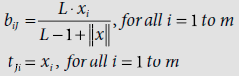
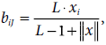
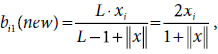
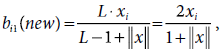
There are various kinds of interconnections in ART1. Each F1(a) input unit Si is connected to the corresponding F1(b) interface unit Xi. There are two types of interconnections between the interface layer F1(b) and the recognition layer F2. The botton-up interconnections are directed from the F1(b) units to F2 units. Each bottom-up interconnection has an weight bij, i = 1, …, m and j = 1,…, n. Similarly, each F2 unit Yj is connected to each F1(b) unit Xi with the help of a top-down interconnection with weight tji, j = 1, …, n and i = 1, …, m. While the bottom-up weights are real valued, the top-down weights are binary. The notations used here relating to ART1 are given in Table 9.6.
Table 9.6. Notational conventions
L |
Learning parameter |
m |
Number of input units (components in the input pattern) |
n |
Maximum number of cluster units (units at layer F2) |
bij |
Bottom-up weight from F1(b) unit Xi to F2 unit Yj, bij is real valued |
tji |
Top-down weight from F2 unit Yj to F1(b) unit Xi, tji is binary |
ρ |
Vigilance parameter |
s |
Training pattern (binary), s = [s1, s2, …, sm] |
x |
x = [x1, x2, …, xm] is the activation vector at the F1(b) layer |
|| x || |
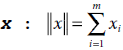
Norm of vector x, |
Learning As stated earlier, ART1 adopts unsupervised learning for clustering binary patterns. It permits the training set of patterns to be presented in any order. The number of clustering units in the recognition layer is flexible. If the net finds a pattern sufficiently different from existing clusters, a new cluster unit is incorporated at the output layer and the concerned pattern is placed in that cluster.
Learning a pattern starts by presenting the pattern to the F1(a) layer which passes it on to the F1(b) layer. F1(b) layer sends it to the F2 layer through the bottom-up interconnection paths. The F2 units compute the net inputs to them. The unit with the largest net input is the winner and has an activation of 1. All other F2 units have 0 activations. The winning F2 unit is the candidate to learn the input pattern. However, it is allowed to do so only if the input pattern is sufficiently close to this cluster.

Fig. 9.16. Algorithm ART1-Learning
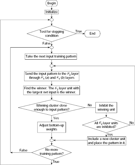
Fig. 9.17. Flow chart of ART1 learning process
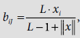
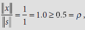
To ensure this, the activation of the winning unit is sent back to F1(b) layer through the top-down interconnections (having binary weights). An F1(b) layer unit remains ‘on’ only if it receives a 1 from both the F1(a) layer and the F2 layer. The norm ||x|| of the vector x at the F1(b) layer gives the number of components where both the F1(a) signal and F2 signal are 1s. The ratio of ||x|| and norm of the input pattern ||s|| gives the degree of similarity between the input pattern and the winning cluster. The ratio ||x||/||s|| is known as the match ratio. If the ratio is sufficiently high, which is determined with the help of the vigilance parameter ρ, the winning cluster is allowed to learn the input pattern. Otherwise, it is inhibited and the net takes appropriate action.
Algorithm ART1–Learning (Fig. 9.16) presents the detailed procedure. The outline of the ART1 learning process is shown in Fig. 9.17 in the form of a flow chart. A few notable points regarding ART1 learning are stated below.
- Learning starts with removing all inhibitions from the units of the clustering layer. This is ensured in Step 4 of Algorithm ART1–Learning by setting the activations of all F2 layer units to 0. An inhibited node has an activation of −1.
- In order to prevent a node from being a winner its activation is set to −1 (Step 12).
- Step 10 ensures that an interface unit Xi is ‘on’ only if si (the training signal) and tJi (the top-down signal sent by the winning unit) are both 1.
- Any one of the following may be used as the stopping condition mentioned in Step 14.
- A predefined maximum number of training epochs have been executed.
- No interconnection weights have changed.
- None of the cluster units resets.
- For the sake of simplicity, the activation of the winning cluster unit is not explicitly made 1. However, the computational procedure implicitly embodies this step and the results are not affected by this omission.
- Step 10 concerns the event of all cluster units being inhibited. The user must specify the action to be taken under such situation. The possible options are
(d) Add more cluster units.
(e) Reduce vigilance.
(f) Classify the pattern as outside of all clusters.
- Table 9.7 shows the permissible range and sample values of various user-defined parameters in ART1 learning.
Table 9.7. ART-1 parameter values

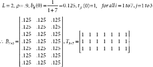
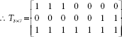
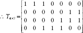
Suppose we want to cluster the patterns [1, 1, 1, 0], [1, 1, 0, 0], [0, 1, 1, 0], [0, 0, 0, 1] and [0, 0, 1, 1] into a maximum of three clusters using the ART-1 learning algorithm. The following set of parameter values are used in this example.
m = 4 |
Number of units in the input layers F1(a) and F1(b) |
n = 3 |
Number of units in the clustering layers F2 |
ρ = 0.5 |
Vigilance parameter |
L = 2 |
Learning parameter, used in updating the bottom-up weights |
Initial bottom-up weights (half of the maximum value allowed) |
|
tji(0) = 1 |
Initial top-down weights (initially all set to 1) |
Execution of the first epoch of ART–1 training is traced below.
Step 0. |
Initialize the learning parameters and the interconnection weights |
|
 |
Step 1. |
Do Steps 2 to 14 While stopping criteria is not satisfied. |
|
/* Epoch No. 1, Pattern No. 1 */ |
Step 2. |
For each training pattern s Do Steps 3 to 13. |
|
Training pattern no. 1 is s = [1, 1, 1, 0] |
Step 3. |
Apply the input pattern s to F1(a) layer, i.e., set the activations of the F1(a) units to the input training pattern s. |
|
Set the activations of the F1(a) units to s = [1, 1, 1, 0]. |
Step 4. |
Set the activations of F2 layer to all 0.
|
|
y1 = y2 = y3 = 0.
|
Step 5. |
Find the norm of s. |
Step 6. |
Propagate input from F1(a) layer to interface layer F1(b) so that xi = si, for all i = 1 to m.
|
|
x = s = [1, 1, 1, 0]
|
Step 7. |
Compute the net inputs to each uninhibited unit of the F2 layer. |
|
For j = 1 To n Do |
|
If yj ≠ −1 Then
|
Step 8. |
While reset is True Do Steps 9 To 12. |
Step 9. |
If yj = −1 for all cluster units, then all of them are inhibited and the pattern cannot be learnt by the net. Otherwise, find the J such that yJ ≥ yj for all j = 1 to n. Then the Jth cluster unit is the winner. In case of a tie, take the smallest J. |
|
None of the cluster units is inhibited and all of them have the same activation value of 0.6. So winner is the lowest indexed unit, so that J = 1. |
Step 10. |
Update x : xi = si× tJi for all i = 1 to m. x = s · T1* = [1, 1, 1, 0] · [1, 1, 1, 1] = [1, 1, 1, 0] |
Step 11. |
Find the norm of  |
Step 12. |
Test for Reset : If |
|
|
Step 13. |
Update the weights (top–down and bottom–up) attached to unit J of the F2 layer. |
|
 |
|
|
|
 |
|
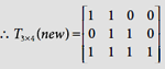
We now update T3×4, the top-down weight matrix. We have, tJi = tli = xi, so that T1*(new) = x = [l, l, l, 0]. |
|
 |
|
This completes training with the first pattern in the first epoch. |
|
/* Epoch No. 1, Pattern No. 2 */ |
Step 2. |
|
|
The second training pattern s = [l, l, 0, 0] |
Step 3. |
Apply the input pattern s to F1(a) layer, i.e., set the activations of the F1(a) units to the input training pattern s. |
|
Set the activations of the F1(a) units to s = [l, l, 0, 0]. |
Step 4. |
Set the activations of F2 layer to all 0.
|
|
y1 = y2 = y3 = 0.
|
Step 5. |
Find the norm of s. |
Step 6. |
Propagate input from F1(a) layer to interface layer F1(b) so that xi = si, for all i = 1 to m.
|
x = s = [1, 1, 0, 0]
|
|
Step 7. |
Compute the net inputs to each uninhibited unit of the F2 layer. |
|
For j = 1 To n Do If yj ≠ −1 Then
|
Step 8. |
|
Step 9. |
If yj = −1 for all cluster units, then all of them are inhibited and the pattern cannot be learnt by the net. Otherwise, find the J such that yJ ≥ yj for all j = 1 to n. Then the Jth cluster unit is the winner. In case of a tie, take the smallest J. |
|
None of the cluster units is inhibited and the cluster unit Y1 has the largest activation 1. So winner is Y1, and J = 1. |
Step 10. |
Update x : xi = si× tJi for all i = 1 to m. x = s · T1* = [1, 1, 0, 0] · [1, 1, 1, 0] = [1, 1, 0, 0]
|
Step 11. |
Find the norm of |
Step 12. |
Test for Reset : If |
|
|
Step 13. |
Update the weights (top–down and bottom–up) attached to unit J of the F2 layer. |
 for all i = 1 to m for all i = 1 to mtJi = xi, for all i = 1 to m
|
|
|
Therefore the new bottom-up weight matrix is |
|
 |
|
We now update T3×4, the top-down weight matrix. We have, tJi = tli = xi, so that T1*(new) = x = [l, l, 0, 0]. |
|
 |
|
This completes training with the second pattern in the first epoch. |
|
/* Epoch No. 1, Pattern No. 3 */ |
Step 2. |
|
|
The third training pattern s = [0, l, l, 0] |
Step 3. |
Apply the input pattern s to F1(a) layer, i.e., set the activations of the F1(a) units to the input training pattern s. |
|
Set the activations of the F1(a) units to [0, l, l, 0]. |
Step 4. |
Set the activations of F2 layer to all 0.
|
|
y1 = y2 = y3 = 0.
|
Step 5. |
Find the norm of s. |
Step 6. |
Propagate input from F1(a) layer to interface layer F1(b) so that xi = si, for all i = 1 to m.
|
|
x = s = [0, l, l, 0]
|
Step 7. |
Compute the net inputs to each uninhibited unit of the F2 layer. |
|
For j = 1 To n Do |
|
|
If yj ≠ −1 Then
|
|
Step 8. |
|
|
Step 9. |
If yj = −1 for all cluster units, then all of them are inhibited and the pattern cannot be learnt by the net. Otherwise, find the J such that yJ ≥ yj for all j = 1 to n. Then the Jth cluster unit is the winner. In case of a tie, take the smallest J. |
|
None of the cluster units is inhibited and the cluster unit Y2 has the largest activation 0.67. So winner is Y2, and J = 2. |
|
Step 10. |
Update x : xi = si×tJi for all i = 1 to m. x = s·T2* = [0, 1, 1, 0] · [1, 1, 1, 1] = [0, 1, 1, 0] |
|
Step 11. |
Find the norm of  |
|
Step 12. |
Test for Reset : If |
|
 hence proceed to Step 13. hence proceed to Step 13. |
|
Step 13. |
Update the weights (top–down and bottom–up) attached to unit J of the F2 layer. |
|
 |
|
| |
|
Therefore the new bottom-up weight matrix is |
|
 |
|
We now update T3×4, the top-down weight matrix. We have, tJi = t2i = xi, so that T2*(new) = x = [0, 1, 1, 0]. |
|
 |
|
This completes training with the third pattern in the first epoch. |
|
/* Epoch No. 1, Pattern No. 4 */ |
Step 2. |
|
|
The fourth training pattern s = [0, 0, 0, 1] |
Step 3. |
Apply the input pattern s to F1(a) layer, i.e., set the activations of the F1(a) units to the input training pattern s. |
|
Set the activations of the F1(a) units to (0, 0, 0, 1). |
Step 4. |
Set the activations of F2 layer to all 0.
|
|
y1 = y2 = y3 = 0.
|
Step 5. |
Find the norm of s. |
Step 6. |
Propagate input from F1(a) layer to interface layer F1(b) so that xi = si, for all i = 1 to m.
|
|
x = s = [0, 0, 0, 1]
|
Step 7. |
Compute the net inputs to each uninhibited unit of the F2 layer. |
|
For j = 1 To n Do |
|
If yj ≠ −1 Then
|
|
Step 8. |
|
Step 9. |
If yj = −1 for all cluster units, then all of them are inhibited and the pattern cannot be learnt by the net. Otherwise, find the J such that yj ≥ yj for all j = 1 to n. Then the Jth cluster unit is the winner. In case of a tie, take the smallest J. |
|
None of the cluster units is inhibited and the cluster unit Y3 has the largest activation 0.2. So winner is Y3, and J = 3. |
Step 10. |
Update x : xi = si×tJi for all i = 1 to m. x = s·T3* = [0, 0, 0, 1]·[1, 1, 1, 1] = [0, 0, 0, 1]
|
Step 11. |
Find the norm of  |
Step 12. |
Test for Reset : If |
|
|
Step 13. |
Update the weights (top–down and bottom–up) attached to unit J of the F2 layer. |
|
 |
|
|
|
Therefore the new bottom-up weight matrix is |
 |
|
|
We now update T3×4, the top-down weight matrix. We have, tJi = t3i = xi, so that T3*(new) = x = [0, 0, 0, 1]. |
|
|
|
This completes training with the fourth pattern in the first epoch. |
|
/* Epoch No. 1, Pattern No. 5 */ |
Step 2. |
|
|
The fifth training pattern s = [0, 0, 1, 1] |
Step 3. |
Apply the input pattern s to F1(a) layer, i.e., set the activations of the F1(a) units to the input training pattern s. |
|
Set the activations of the F1(a) units to [0, 0, 1, 1]. |
Step 4. |
Set the activations of F2 layer to all 0.
|
|
y1 = y2 = y3 = 0.
|
Step 5.
|
Find the norm of s. |
Step 6. |
Propagate input from F1(a) layer to interface layer F1(b) so that xi = si, for all i = 1 to m.
|
|
x = s = [0, 0, 1, 1]
|
Step 7. |
Compute the net inputs to each uninhibited unit of the F2 layer. |
|
For j = 1 To n Do If yj ≠ −1 Then
 |
Step 9. |
If yj = −1 for all cluster units, then all of them are inhibited and the pattern cannot be learnt by the net. Otherwise, find the J such that yJ ≥ yj for all j = 1 to n. Then the Jth cluster unit is the winner. In case of a tie, take the smallest J. |
|
None of the cluster units is inhibited and the cluster unit Y3 has the largest activation 1. So winner is Y3, and J = 3. |
Step 10. |
Update x : xi = si× tJi for all i = 1 to m. x = s·T3* = [0, 0, 1, 1]·[0, 0, 0, 1] = [0, 0, 0, 1] |
Step 11. |
Find the norm of
 |
Step 12. |
Test for Reset : If |
|
|
Step 13. |
Update the weights (top–down and bottom–up) attached to unit J of the F2 layer. |
|
 for all i = 1 to m for all i = 1 to mtJi = xi, for all i = 1 to m
|
|
Therefore the new bottom-up weight matrix is |
|
 |
We now update T3×4, the top-down weight matrix. We have, tJi = t3i = xi, so that T3*(new) = x = [0, 0, 0, 1]. |
|
|
 |
|
This completes training with the fifth pattern in the first epoch. |
Step 14. |
Test for stopping condition. |
|
The reader may verify that this set of weights is stable and no learning takes place even on further training with the given set of patterns. |

 hence proceed to Step 13.
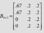
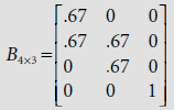
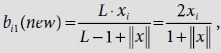 ∴ b11(new) = b21(new) = b31(new) = 0.5, and b41(new) = 0. Therefore the new bottom-up weight matrix is
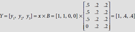
 hence proceed to
  ∴ b11(new) = b21(new) = .67, b31(new) = b41(new) = 0.
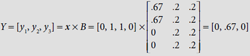
 and proceed to
 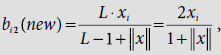 ∴ b22(new) = b32(new) = .67, b12(new) = b42(new) = 0.
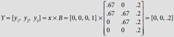
 hence proceed to
  ∴ b13(new) = b23(new) = b33(new) = 0, b43(new) = 1.
 hence proceed to
  ∴ b13(new) = b23(new) = b33(new) = 0, b43(new) = 1.
Example 9.6 (ART1 net operation)
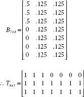
Let us consider an ART-1 net with 5 input units and 3 cluster units. After some training the net attains the bottom-up and top-down weight matrices as shown below.

Show the behaviour of the net if it is presented with the training pattern s = [0, 1, 1, 1, 1]. Assume L = 2, and ρ = .8.
We start the training process from Step 2 of the ATR-1 learning procedure.
Step 2. |
For each training pattern s Do Steps 3 to 13.
|
|
Here s = [0, 1, 1, 1, 1]
|
Step 3. |
Apply the input pattern s to F1(a) layer, i.e., set the activations of the F1(a) units to the input training pattern s. |
|
Set the activations of the F1(a) units to [0, 1, 1, 1, 1]. |
Step 4. |
Set the activations of F2 layer to all 0.
|
|
y1 = y2 = y3 = 0.
|
Step 5. |
Find the norm of |
Step 6. |
Propagate input from F1(a) layer to interface layer F1(b) so that xi = si, for all i = 1 to m.
|
|
x = s = [0, 1, 1, 1, 1]
|
Compute the net inputs to each uninhibited unit of the F2 layer. |
|
|
For j = 1 To n Do |
|
If yj ≠ −1 Then
|
Step 8. |
|
Step 9. |
If yj = −1 for all cluster units, then all of them are inhibited and the pattern cannot be learnt by the net. Otherwise, find the J such that yJ ≥ yj for all j = 1 to n. Then the Jth cluster unit is the winner. In case of a tie, take the smallest J. |
|
None of the cluster units is inhibited and the cluster unit Y2 has the largest activation 1.6. So winner is Y2, and J = 2. |
Step 10. |
Update x : xi = si× tJi for all i = 1 to m. x = s·T2* = [0, 1, 1, 1, 1]·[0, 1, 1, 1, 0] = [0, 1, 1, 1, 0] |
Step 11. |
Find the norm of  |
Step 12. |
Test for Reset : If |
|
|
Step 8. |
|
If yj = −1 for all cluster units, then all of them are inhibited and the pattern cannot be learnt by the net. Otherwise, find the J such that yJ ≥ yj for all j = 1 to n. Then the Jth cluster unit is the winner. In case of a tie, take the smallest J. |
|
|
Since Y2 is inhibited, we have [y1, y2, y3] = [1.6,−1, .8]. Therefore unit Y1 has the largest activation 1.6 and winner is Y1, so that J = 1. |
Step 10. |
Update x : xi = si×tJi for all i = 1 to m. x = s·T1* = [0, 1, 1, 1, 1]·[1, 1, 1, 1, 1] = [0, 1, 1, 1, 1]
|
Step 11. |
Find the norm of  |
Step 12. |
Test for Reset : If |
|
|
Step 13. |
Update the weights (top–down and bottom–up) attached to unit J of the F2 layer. |
|
 for all i = 1 to m for all i = 1 to mtJi = xi, for all i = 1 to m
|
|
|
|
Therefore the new bottom-up weight matrix is |
|
 |
We now update T3×5, the top-down weight matrix. We have, tJi = t1i = xi, so that T1*(new) = x = [0, 1, 1, 1, 1]. |
|
 |


 ∴ b11(new) = 0, and b21(new) = b31(new) = b41(new) = b51(new) = .4.
This completes training with the given pattern s = (0, 1, 1, 1, 1).
CHAPTER SUMMARY
Basic concepts of competitive networks and brief descriptions of certain elementary competitive networks are discussed in this chapter. The main points are summarized below.
- A competitive neural net is a clustering net that selects the output clustering unit through competition. Usually the competition is in terms of the distance between the input pattern and the weight vector associated with the output unit. Quite frequently, the distance is measured either as the Euclidean distance between two points in a hyperplane or the dot product of the input vector and the weight vector.
- MAXNET is the simplest competitive ANN. It is a fully connected network with symmetric interconnections and self-loops. All the links have the same, fixed, inhibitory weight –δ. Each unit has a self-loop. The weight of a self-loop is 1. A MAXNET do not required to be trained because all weights are fixed. During application, as the MAXNET is presented with an input vector, it iteratively updates the activations of the cluster units until all units except one are deactivated. The only remaining positively activated unit is the winner.
- Kohonen’s self-organizing map (SOM) works on the principle of winner-takes-all and follows unsupervised learning. Here the weight vector associated with a cluster unit acts as the exemplar. During learning, the cluster unit whose weight vector is closest to the given input pattern is declared the winner. The weight vectors of all cluster units in the neighbourhood of the winner are updated. During application, the input pattern is compared with the exemplar / code vector. The unit whose code vector is at a least distance from the input pattern is the winner.
- Learning Vector Quantization (LVQ) nets are also based on the winner-takes-all strategy, though, unlike Kohonen’s SOM, LVQ follows supervised learning. There are as many input units as the number of components in the input patterns and each output unit represents a known cluster. During each epoch of training, the LVQ net adjusts its weights to accommodate the training vectors on the basis of the known clusters. During training, the net identifies the code vector w closest to the input vector s. If s and w are from the same cluster, then w is moved closer to s. Otherwise, w is moved away from x. During application, the cluster unit whose code vector is at a least distance from the input pattern is the winner.
- Adaptive Resonance Theory (ART) nets were introduced to resolve the stability-plasticity dilemma. These nets learn through unsupervised learning where the input patterns may be presented in any order. Moreover, ART nets allow the user to control the degree of similarity among the patterns placed in the same cluster. It provides a mechanism to include a new cluster unit for an input pattern which is sufficiently different from all the exemplars of the clusters corresponding to the existing cluster units. Hence, unlike other ANNs, ART nets are capable of adaptive expansion of the output layer of clustering units subject to some upper bound. ART nets are able to learn only in their resonant states. The ART net is in resonant state when the current input vector matches the winner code-vector (exemplar) so close that a reset signal is not generated. The reset signal inhibits the ART to learn. There are two kinds of ARTs, viz., ART1 and ART2. ART1 works on binary patterns and ART2 is designed for patterns with real, or continuous, values.
SOLVED PROBLEMS
Problem 9.1 (Clustering application of SOM) Consider the SOM constructed in Example 9.2. The weight matrix of the resultant SOM is given by

Fig. 9.18 shows the SOM obtained for the given clustering problem.
Fig. 9.18. The SOM obtained in Example 9.2
Test the performance of this net with the input vectors [1, 0, 0], [0, 0, 1], [1, 1, 0] and [0, 1, 1].
Solution 9.1 Table 9.8 shows the calculations to identify the cluster to which each vector belongs, the decision being made on the basis of Winner-takes-all policy. It is seen that the SOM clusters the patterns (1, 0, 0) and (1, 1, 0) at unit C2 and the patterns (0, 0, 1) and (0, 1, 1) at unit C1 (Fig. 9.19). Considering the relative positions of the vectors in a 3-dimensional space, this is the correct clustering for these patterns.
Table 9.8. Calculations to identify the cluster


Problem 9.2 (Creating and training an ART1 net) Create an ART-1 net initially with 7 inputs and 3 clusters. Then apply the ART-1 procedure to train the net with the following patterns: [1, 1, 1, 1, 0, 0, 0], [1, 1, 1, 0, 0, 0, 0], [0, 0, 0, 0, 0, 1, 1], [0, 0, 0, 0, 1, 1, 1], [0, 0, 1, 1, 1, 0, 0] and [0, 0, 0, 1, 0, 0, 0].
Solution 9.2 Execution of the first epoch of ART-1 training is traced below.
Step 0. |
Initialize the learning parameters and the interconnection weights |
|
 |
Step 1. |
Do Steps 2 to 14 While stopping criteria is not satisfied. |
|
/* Epoch No. 1, Pattern No. 1 */ |
Step 2. |
For each training pattern s Do Steps 3 to 13. |
|
The fifth training pattern s = [1, 1, 1, 1, 0, 0, 0] |
Step 3. |
Apply the input pattern s to F1(a) layer, i.e., set the activations of the F1(a) units to the input training pattern s. |
|
Set the activations of the F1(a) units to [1, 1, 1, 1, 0, 0, 0]. |
Step 4. |
Set the activations of F2 layer to all 0.
|
|
y1 = y2 = y3 = 0.
|
Step 5. |
Find the norm of s. |
Propagate input from F1(a) layer to interface layer F1(b) so that xi = si, for all i = 1 to m.
|
|
|
x = s = [1, 1, 1, 1, 0, 0, 0]
|
Step 7. |
Compute the net inputs to each uninhibited unit of the F2 layer. |
|
For j = 1 To n Do |
|
If yj ≠ −1 Then
|
Step 8. |
While reset is True Do Steps 9 To 12. |
Step 9. |
If yj = −1 for all cluster units, then all of them are inhibited and the pattern cannot be learnt by the net. Otherwise, find the J such that yJ ≥ yj for all j = 1 to n. Then the Jth cluster unit is the winner. In case of a tie, take the smallest J. |
|
None of the cluster units is inhibited and all of them have the same activation value of 0.5. So the winner is the lowest indexed unit, so that J = 1. |
Step 10. |
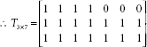
Update x : xi = si×tJi for all i = 1 to m. x = s·T1* = [1, 1, 1, 1, 0, 0, 0] · [1, 1, 1, 1, 1, 1, 1] = [1, 1, 1, 1, 0, 0, 0].
|
Step 11. |
Find the norm of |
Step 12. |
Test for Reset : If |
|
|
Step 13. |
Update the weights (top–down and bottom–up) attached to unit J of the F2 layer. |
|
 for all i = 1 to m for all i = 1 to mtJi = xi, for all i = 1 to m
|
|
|
|
Therefore the new bottom-up weight matrix is |
|
 |
|
We now update T3×7, the top-down weight matrix. We have, tJi = t1i = xi, so that T1*(new) = x = [1, 1, 1, 1, 0, 0, 0]. |
|
 |
|
This completes training with the first pattern in the first epoch. |
|
/* Epoch No. 1, Pattern No. 2 */ |
Step 2. |
|
|
The second training pattern s = [1, 1, 1, 0, 0, 0, 0] |
Step 3. |
Apply the input pattern s to F1(a) layer, i.e., set the activations of the F1(a) units to the input training pattern s. |
|
Set the activations of the F1(a) units to [1, 1, 1, 0, 0, 0, 0]. |
Step 4. |
Set the activations of F2 layer to all 0.
|
|
y1 = y2 = y3 = 0.
|
Step 5. |
Find the norm of s. |
Propagate input from F1(a) layer to interface layer F1(b) so that xi = si, for all i = 1 to m.
|
|
|
x = s = [1, 1, 1, 0, 0, 0, 0]
|
Step 7. |
Compute the net inputs to each uninhibited unit of the F2 layer. For j = 1 To n Do |
|
|
If yj ≠ −1 Then
= [1.2, .375, .375] |
Step 8. |
|
Step 9. |
If yj = −1 for all cluster units, then all of them are inhibited and the pattern cannot be learnt by the net. Otherwise, find the J such that yJ ≥ yj for all j = 1 to n. Then the Jth cluster unit is the winner. In case of a tie, take the smallest J. |
|
None of the cluster units is inhibited and y1 has the highest activation value of 1.2. So winner is the lowest indexed unit Y1, so that J = 1. |
Step 10. |
Update x : xi = si×tJi for all i = 1 to m. x = s·T1* = [1, 1, 1, 0, 0, 0, 0] · [1, 1, 1, 1, 0, 0, 0] = [1, 1, 1, 0, 0, 0, 0].
|
Step 11. |
Find the norm of |
Step 12. |
Test for Reset : If |
|
|
Step 13. |
Update the weights (top–down and bottom–up) attached to unit J of the F2 layer. |
|
 for all i = 1 to m for all i = 1 to mtJi = xi, for all i = 1 to m
|
|
|
|
Therefore the new bottom-up weight matrix is |
|
 |
|
We now update T3×7, the top-down weight matrix. We have, tJi = t1i = xi, so that T1*(new) = x = [1, 1, 1, 0, 0, 0, 0]. |
|
 |
|
This completes training with the second pattern in the first epoch. |
|
/* Epoch No. 1, Pattern No. 3 */ |

 ∴ b11(new) = b21(new) = b31(new) = b41(new) = 0.4, and b51(new) = b61(new) = b71(new) = 0.
 ∴ b11(new) = b21(new) = b31(new) = 0.5, and b41(new) = b51(new) = b61(new) = b71(new) = 0.
Similarly, training with the third training pattern s = [0, 0, 0, 0, 0, 1, 1] yields the bottom-up and top-down weight matrices as follows:

Now we proceed to train with the fourth pattern [0, 0, 0, 0, 1, 1, 1].
|
/* Epoch No. 1, Pattern No. 4 */ |
Step 2. |
|
|
The fourth training pattern s = [0, 0, 0, 0, 1, 1, 1] |
Step 3. |
Apply the input pattern s to F1(a) layer, i.e., set the activations of the F1(a) units to the input training pattern s. |
|
Set the activations of the F1(a) units to [0, 0, 0, 0, 1, 1, 1]. |
Step 4. |
Set the activations of F2 layer to all 0.
|
|
y1 = y2 = y3 = 0.
|
Step 5. |
Find the norm of s. |
Step 6. |
Propagate input from F1(a) layer to interface layer F1(b) so that xi = si, for all i = 1 to m.
|
|
x = s = [0, 0, 0, 0, 1, 1, 1]
|
Step 7. |
Compute the net inputs to each uninhibited unit of the F2 layer. |
|
For j = 1 To n Do |
|
|
If yj ≠ −1 Then
= [0, .1.34, .375] |
Step 8. |
|
If yj = −1 for all cluster units, then all of them are inhibited and the pattern cannot be learnt by the net. Otherwise, find the J such that yJ ≥ yj for all j = 1 to n. Then the Jth cluster unit is the winner. In case of a tie, take the smallest J. |
|
|
None of the cluster units is inhibited and y2 has the highest activation value of 1.34. So winner is the lowest indexed unit Y2, so that J = 2. |
Step 10. |
Update x : xi = si × tJi for all i = 1 to m. x = s·T2* = [0, 0, 0, 0, 1, 1, 1] · [0, 0, 0, 0, 0, 1, 1] = [0, 0, 0, 0, 0, 1, 1].
|
Step 11. |
Find the norm of 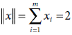 |
Step 12. |
Test for Reset : If |
|
|
Step 9. |
If yj = −1 for all cluster units, then all of them are inhibited and the pattern cannot be learnt by the net. Otherwise, find the J such that yJ ≥ yj for all j = 1 to n. Then the Jth cluster unit is the winner. In case of a tie, take the smallest J. |
|
Cluster units Y2 is inhibited and between Y1and Y3, Y3 has the highest activation value of 0.375. So winner is the lowest indexed unit Y3, so that J = 3. |
Step 10. |
Update x : xi = si×tJi for all i = 1 to m. x = s·T3* = [0, 0, 0, 0, 1, 1, 1] · [1, 1, 1, 1, 1, 1, 1] = [0, 0, 0, 0, 1, 1, 1]. |
Step 11. |
Find the norm of |
Test for Reset : If |
|
|
|
Step 13. |
Update the weights (top–down and bottom–up) attached to unit J of the F2 layer. |
|
 for all i = 1 to m for all i = 1 to mtJi = xi, for all i = 1 to m
|
|
|
|
Therefore the new bottom-up weight matrix is |
|
 |
|
We now update T3×7, the top-down weight matrix. We have, tJi = t1i = xi, so that T3* (new) = x = [0, 0, 0, 0, 1, 1, 1]. |
|
 |
|
This completes training with the fourth pattern in the first epoch. |
|
/* Epoch No. 1, Pattern No. 5 */ |
Step 2. |
|
|
The fifth training pattern is s = [0, 0, 1, 1, 1, 0, 0] |
Step 3. |
Apply the input pattern s to F1(a) layer, i.e., set the activations of the F1(a) units to the input training pattern s. |
|
Set the activations of the F1(a) units to (0, 0, 1, 1, 1, 0, 0). |
Set the activations of F2 layer to all 0.
|
|
|
y1 = y2 = y3 = 0.
|
Step 5. |
Find the norm of s. |
Step 6. |
Propagate input from F1(a) layer to interface layer F1(b) so that xi = si, for all i = 1 to m.
|
|
x = s = [0, 0, 1, 1, 1, 0, 0]
|
Step 7. |
Compute the net inputs to each uninhibited unit of the F2 layer. |
|
For j = 1 To n Do |
|
If yj ≠ −1 Then  = [.5, 0, .5]
|
Step 8. |
|
Step 9. |
If yj = −1 for all cluster units, then all of them are inhibited and the pattern cannot be learnt by the net. Otherwise, find the J such that yJ ≥ yj for all j = 1 to n. Then the Jth cluster unit is the winner. In case of a tie, take the smallest J. |
|
None of the cluster units is inhibited and both Y1 and Y3 has the highest activation value of .5. So winner is the lowest indexed unit Y1, so that J = 1. |
Step 10. |
Update x : xi = si×tJi for all i = 1 to m. x = s·T1* = [0, 0, 1, 1, 1, 0, 0] · [1, 1, 1, 0, 0, 0, 0] = [0, 0, 1, 0, 0, 0, 0].
|
Step 11. |
Find the norm of |
Step 12. |
Test for Reset : If |
|
|
Step 9. |
If yj = −1 for all cluster units, then all of them are inhibited and the pattern cannot be learnt by the net. Otherwise, find the J such that yJ ≥ yj for all j = 1 to n. Then the Jth cluster unit is the winner. In case of a tie, take the smallest J. |
|
Cluster unit Y1 is inhibited and between Y2 and Y3, Y3 has the highest activation value of 0.5. So winner is the lowest indexed unit Y3, and J = 3. |
Step 10. |
Update x : xi = si×tJi for all i = 1 to m. x = s·T3* = [0, 0, 1, 1, 1, 0, 0] · [0, 0, 0, 0, 1, 1, 1] = [0, 0, 0, 0, 1, 0, 0].
|
Step 11. |
Find the norm of |
Step 12. |
Test for Reset : If |
|
|
Step 9. |
If yj = −1 for all cluster units, then all of them are inhibited and the pattern cannot be learnt by the net. Otherwise, find the J such that yJ ≥ yj for all j = 1 to n. Then the Jth cluster unit is the winner. In case of a tie, take the smallest J. |
Cluster units Y1 and Y3 are inhibited so that Y2 has the highest activation value of 0. So winner is the unit Y2, so that J = 2. |
|
Step 10. |
Update x : xi = si×tJi for all i = 1 to m. x = s·T2* = [0, 0, 1, 1, 1, 0, 0] · [0, 0, 0, 0, 0, 1, 1] = [0, 0, 0, 0, 0, 0, 0]. |
Step 11. |
Find the norm of |
Step 12. |
Test for Reset : If |
|
|
Step 9. |
If yj = −1 for all cluster units, then all of them are inhibited and the pattern cannot be learnt by the net. Otherwise, find the J such that yJ ≥ yj for all j = 1 to n. Then the Jth cluster unit is the winner. In case of a tie, take the smallest J. |
|
All cluster units are now inhibited. So we introduce a new cluster unit Y4. The modified bottom-up and top-down weight matrices are now: |
|
 |
|
As the cluster units Y1, Y2, and Y3 are all inhibited the remaining new unit Y4 has the highest activation value of 0.375. So winner is the unit Y4, so that J = 4. |
Step 10. |
Update x : xi = si×tJi for all i = 1 to m. |
x = s·T4* = [0, 0, 1, 1, 1, 0, 0] · [1, 1, 1, 1, 1, 1, 1] = [0, 0, 1, 1, 1, 0, 0].
|
|
Step 11. |
Find the norm of |
Step 12. |
Test for Reset : If |
|
|
Step 13. |
Update the weights (top–down and bottom–up) attached to unit J of the F2 layer. |
|
tJi = xi, for all i = 1 to m
|
|
|
|
Therefore the new bottom-up weight matrix is |
|
 |
|
We now update T4×7, the top-down weight matrix. We have, tJi = t1i = xi, so that T4* (new) = x = [0, 0, 1, 1, 1, 0, 0]. |
|
 |

 ∴ b13(new) = b23(new) = b33(new) = b43(new) = 0. b53(new) = b63(new) = b73(new) = 0.5.
 ∴ b14(new) = b24(new) = b64(new) = b74(new) = 0. b34(new) = b44(new) = b54(new) = 0.5.
This completes training with the fifth pattern in the first epoch.
Training with the last pattern (0, 0, 0, 1, 0, 0, 0) is left as an exercise. We will see that none of the existing four cluster units is able to learn this pattern. Providing one more cluster unit Y5 to accommodate this pattern, we finally have

Problem 9.3 (Creating and training an ART1 net) Repeat the previous problem with ρ = .3.
Solution 9.3 The ART-1 net initially consists of 7 inputs and 3 clusters. The training set comprises the patterns: [1, 1, 1, 1, 0, 0, 0], [1, 1, 1, 0, 0, 0, 0], [0, 0, 0, 0, 0, 1, 1], [0, 0, 0, 0, 1, 1, 1], [0, 0, 1, 1, 1, 0, 0] and [0, 0, 0, 1, 0, 0, 0]. The vigilance parameter ρ = .3. Execution of the first epoch of ART-1 training is traced below.
Step 0. |
Initialize the learning parameters and the interconnection weights |
|
|
 |
|
Step 1. |
Do Steps 2 to 14 While stopping criteria is not satisfied. |
|
|
/* Epoch No. 1, Pattern No. 1 */ |
|
|
This is same in the previous example. The new bottom-up weight matrix and the top-down weight matrix at the end of training with the first pattern are |
|
 |
||
|
/* Epoch No. 1, Pattern No. 2 */ |
|
|
The training is again same as in the previous example. The resultant bottom-up and top-down weight matrices are given by |
|
|
 |
|
|
Similarly, the bottom-up and top-down weight matrices after training with the third pattern in the first epoch are given by |
|
|
 |
|
Now we proceed to train with the fourth pattern [0, 0, 0, 0, 1, 1, 1]. |
||
|
/* Epoch No. 1, Pattern No. 4 */ |
|
Step 2. |
For each training pattern s Do Steps 3 to 13. |
|
|
The fourth training pattern s = [0, 0, 0, 0, 1, 1, 1] |
|
Step 3. |
Apply the input pattern s to F1(a) layer, i.e., set the activations of the F1(a) units to the input training pattern s. |
|
|
Set the activations of the F1(a) units to [0, 0, 0, 0, 1, 1, 1]. |
|
Step 4. |
Set the activations of F2 layer to all 0.
|
|
|
y1 = y2 = y3 = 0.
|
|
Step 5. |
Find the norm of s. |
|
Step 6. |
Propagate input from F1(a) layer to interface layer F1(b) so that xi = si, for all i = 1 to m.
|
|
|
x = s = [0, 0, 0, 0, 1, 1, 1]
|
|
Step 7. |
Compute the net inputs to each uninhibited unit of the F2 layer. |
|
|
For j = 1 To n Do |
|
|
If yj ≠ −1 Then 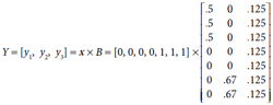 = [0, .1.34, .375]
|
|
Step 8. |
While reset is True Do Steps 9 To 12. |
|
Step 9. |
If yj = −1 for all cluster units, then all of them are inhibited and the pattern cannot be learnt by the net. Otherwise, find the J such that yJ ≥ yj for all j = 1 to n. Then the Jth cluster unit is the winner. In case of a tie, take the smallest J. |
|
None of the cluster units is inhibited and y2 has the highest activation value of 1.34. So winner is the lowest indexed unit Y2, so that J = 2. |
||
Step 10. |
Update x : xi = si×tJi for all i = 1 to m. x = s·T2* = [0, 0, 0, 0, 1, 1, 1] · [0, 0, 0, 0, 0, 1, 1] = [0, 0, 0, 0, 0, 1, 1].
|
|
Step 11. |
Find the norm of |
|
Step 12. |
Test for Reset : If |
|
|
|
|
Step 13. |
Update the weights (top–down and bottom–up) attached to unit J of the F2 layer. |
|
|
 for all i = 1 to m for all i = 1 to mtJi = xi, for all i = 1 to m
|
|
|
|
|
|
Therefore there is no change in the new bottom-up weight matrix and top-down weight matrix. |
|
|
 |
|
|
This completes training with the fourth pattern in the first epoch. |
|
/* Epoch No. 1, Pattern No. 5 */ |
||
Step 2. |
||
|
The fifth training pattern s = [0, 0, 1, 1, 1, 0, 0] |
|
Step 3. |
Apply the input pattern s to F1(a) layer, i.e., set the activations of the F1(a) units to the input training pattern s. |
|
|
Set the activations of the F1(a) units to [0, 0, 1, 1, 1, 0, 0]. |
|
Step 4. |
Set the activations of F2 layer to all 0.
|
|
|
y1 = y2 = y3 = 0.
|
|
Step 5. |
Find the norm of s. |
|
Step 6. |
Propagate input from F1(a) layer to interface layer F1(b) so that xi = si, for all i = 1 to m.
|
|
|
x = s = [0, 0, 1, 1, 1, 0, 0]
|
|
Step 7. |
Compute the net inputs to each uninhibited unit of the F2 layer. |
|
|
For j = 1 To n Do |
|
|
If yj ≠ −1 Then  = [.5, 0, .375] |
|
Step 8. |
||
Step 9. |
If yj = −1 for all cluster units, then all of them are inhibited and the pattern cannot be learnt by the net. Otherwise, find the J such that yJ ≥ yj for all j = 1 to n. Then the Jth cluster unit is the winner. In case of a tie, take the smallest J. |
|
|
None of the cluster units is inhibited and Y1 has the highest activation value of .5. So winner is the lowest indexed unit Y1, so that J = 1. |
|
|
Update x : xi = si× tJi for all i = 1 to m. x = s·T1* = [0, 0, 1, 1, 1, 0, 0] · [1, 1, 1, 0, 0, 0, 0] = [0, 0, 1, 0, 0, 0, 0].
|
||
Step 11. |
Find the norm of |
|
Step 12. |
Test for Reset : If |
|
|
|
|
Step 13. |
Update the weights (top–down and bottom–up) attached to unit J of the F2 layer. |
|
|
 for all i = 1 to m for all i = 1 to mtJi = xi, for all i = 1 to m
|
|
|
|
|
|
Therefore the new bottom-up weight matrix is |
|
|
 |
|
|
This completes training with the fifth pattern in the first epoch. |
|
|
/* Epoch No. 1, Pattern No. 6 */ |
|
Step 2. |
||
|
The sixth training pattern s = [0, 0, 0, 1, 0, 0, 0] |
|
Apply the input pattern s to F1(a) layer, i.e., set the activations of the F1(a) units to the input training pattern s. |
||
|
Set the activations of the F1(a) units to [0, 0, 0, 1, 0, 0, 0]. |
|
Step 4. |
Set the activations of F2 layer to all 0.
|
|
|
y1 = y2 = y3 = 0.
|
|
Step 5. |
Find the norm of s. |
|
Step 6. |
Propagate input from F1(a) layer to interface layer F1(b) so that xi = si, for all i = 1 to m.
|
|
|
x = s = [0, 0, 0, 1, 0, 0, 0]
|
|
Step 7. |
Compute the net inputs to each uninhibited unit of the F2 layer. |
|
|
For j = 1 To n Do |
|
|
If yj ≠ −1 Then 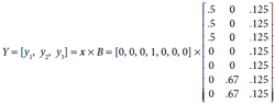 = [0, 0, .125]
|
|
Step 8. |
||
Step 9. |
If yj = −1 for all cluster units, then all of them are inhibited and the pattern cannot be learnt by the net. Otherwise, find the J such that yJ ≥ yj for all j = 1 to n. Then the Jth cluster unit is the winner. In case of a tie, take the smallest J. |
|
|
None of the cluster units is inhibited and Y3 has the highest activation value of .125. So winner is the lowest indexed unit Y3, so that J = 3. |
|
Step 10. |
Update x : xi = si×tJi for all i = 1 to m. x = s·T3* = [0, 0, 0, 1, 0, 0, 0] · [1, 1, 1, 1, 1, 1, 1] = [0, 0, 0, 1, 0, 0, 0].
|
|
Step 11. |
Find the norm of |
|
Test for Reset : If |
||
|
|
|
Step 13. |
Update the weights (top–down and bottom–up) attached to unit J of the F2 layer. |
|
|
 for all i = 1 to m for all i = 1 to mtJi = xi, for all i = 1 to m
|
|
|
|
|
|
Therefore the new bottom-up weight matrix is |
|
|
 |
|
|
This completes training with the sixth pattern in the first epoch. |


 ∴ b12(new) = b22(new) = b32(new) = b42(new) = b52(new) = 0. b62(new) = b72(new) = 0.67.
 ∴ b11(new) = b21(new) = b41(new) = b51(new) = b61(new) = b71(new) = 0, b34(new) = 1.
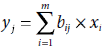
 ∴ b13(new) = b23(new) = b33(new) = b53(new) = b63(new) =
b73(new) = 0, = b43(new) = 1.
∴ b13(new) = b23(new) = b33(new) = b53(new) = b63(new) =
b73(new) = 0, = b43(new) = 1.
Problem 9.4 (Implementation of LVQ net through MatLab) Write a MatLab program to design and implement an LVQ net with two inputs and two outputs. The two outputs should correspond to two clusters, cluster 1 and cluster 2. The training set consists of the training pairs { [0 –2] : 1, [+2 –1] : 1, [–2 +1] : 1, [0 +2] : 2, [+1 +1] : 2, [0 +1] : 2, [+1 +3] : 2, [–3 +1] : 1, [3 –1] : 1, [–3, 0] : 1}. Test the net with the input pattern [0.2, –1].
Solution 9.4 The MatLab code for the net, its training and testing, is given below.
****************** CODE FOR LEARNING VECTOR QUANTIZATION NETWORKS***********
clc;
clear;
Input_Vector = [0 +2 −2 0 +1 0 +1 −3 3 −3;
−2 −1 +1 +2 +1 +1 +3 +1 −1 0];
% Input Vector comsists of 10 samples having 2 inputs each.
Target_Class = [1 1 1 2 2 2 2 1 1 1];
% The Input Vector has to be classified into two classes, namely Class 1
% and Class 2. 6 inputs belong to Class 1 and 4 belong to Class 2.
Target_Vector = ind2vec(Target_Class);
% Converting indices to vector
net = newlvq(minmax(Input_Vector),4,[.6 .4],0.1);
% Creating new LVQ network. The network takes input from P, has 4 hidden
% neurons and two classes having percentages of 0.6 and 0.4 respectively.
% The learning rate is 0.1.
net.trainParam.epochs = 150; % Setting maximum number of epochs to 150
net=train(net,Input_Vector,Target_Vector); % Train the network
Test_Vector_1 = [0.2; 1];
a = vec2ind(sim(net, |
% Simulate network with test vector |
disp('Test_Vector_1 [0.2; 1] has been classified as belonging to Class –'),
disp(a);
Test_Vector_2 = [0.2; −1];
a = vec2ind(sim(net,Test_Vector_2));
disp('Test_Vector_2 [0.2; −1] has been classified as belonging to Class−'),
disp(a);
***********************************OUTPUT*************************************
Test_Vector_1 [0.2; 1] has been classified as belonging to Class - 2
Test_Vector_2 [0.2; −1] has been classified as belonging to Class - 1
Problem 9.5 (Self-organizing maps) The Iris dataset on flowers consists of 150 sample data. It is based on four attributes, sepal length in cm, sepal width in cm, petal length in cm, and petal width in cm, along with the type of flower. This dataset can be copied from the webpage http://mlg.eng.cam.ac.uk/teaching/3f3/1011/iris.data or downloaded from: http://www2.acae.cuhk.edu.hk/~cvl/main_database.htm. Design a SOM in MatLab for this dataset.
Solution 9.5 The MatLab code along with various outputs are given below.
MatLab code
% |
SOM on Iris Data Set mds3.txt |
% |
Classify iris flowers based on four attributes. |
% |
The data set consists of 150 samples. |
% |
“irisInputs” is an 4x150 matrix, whose rows are: |
% |
1. Sepal length in cm |
% |
2. Sepal width in cm |
% |
3. Petal length in cm |
% |
4. Petal width in cm |
clc;
clear();
load mdstrain.txt; |
% Load the training file containing 150 samples |
|
% having 4 fields |
r = mdstrain(:,1:4); |
% Bring the contents of the text file to matrix |
r |
|
r = r'; |
% Transpose r to bring in order of rows |
net = newsom(r,[10 10]); |
% Create new SOM for r with 10 x 10 hidden |
|
% neurons. The other parameters are kept at |
|
% default values. |
% |
The syntax for newsom is net = newsom(P,[D1,D2,...],TFCN, DFCN, STEPS, IN) |
% |
where P = R × Q matrix of Q representative input vectors. |
% |
Di = Size of ith layer dimension. Defaults = [5 8]. Here it is [10 10] |
% |
TFCN = Topology function. Default = 'hextop'. May be made 'gridtop' or |
% |
'randtop' |
% |
DFCN = Distance function. Default = 'linkdist'. Can be made 'dist' or |
% |
'mandist'. 'linkdist' is a layer distance function used to find the |
% |
distances between the layer's neurons given their positions.'dist' is the Eucledian distance function while 'mandist' is the Manhattan distance function. |
% |
STEPS = Steps for neighborhood to shrink to 1. Default = 100. |
% |
IN = Initial neighborhood size. default = 3. |
net = train(net,r); |
% Train the network. train(net,r) opens up the |
|
% nntraintool from which the plots can be |
|
% generated. |
Snapshots of MatLab outputs

Fig. 9.20. The ‘nntraintool’ window of MatLab
Various SOM profiles are generated by clicking the respective buttons on the nntraintool. These are shown below as Fig. 9.21–9.26

Fig. 9.21. SOM Topology, plotted by function ‘plotsomtop’.
This shows the topology of the SOM

Fig. 9.22. SOM neighbor connections, plotted by the function ‘plotsomnc’. This plot shows the SOM layer, with the neurons denoted as dark patches and their connections with their direct neighbours denoted as line segments.
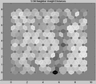
Fig. 9.23. SOM neighbor weight distances, plotted by the function ‘plotsomnd’. This plot depicts the SOM layer with the neurons as standard dark central patches and their direct neighbour relations with line segments. The neighbouring patches are presented here with various shades of grey to show how close each neuron’s weight vector is to its neighbours.

Fig. 9.24. SOM weight planes, plotted by the function ‘plotsomplanes’. The ‘plotsomplanes’ generates a set of subplots where each subplot shows the weights from the i-th input to the layer’s neurons. The various connections are shown with different shades of grey (black for zero connection)

Fig. 9.25. SOM sample hits, plotted by function ‘plotsomhits’. This plot shows a SOM layer, with each neuron and the number of input vectors that are classified by it. This is shown as a number inside the cells.

Fig. 9.26. SOM weight positions, plotted by function ‘plotsompos’. This plot shows how the classification of the input space is done by the SOM. It shows dots for each neuron’s weight vector and the connecting neighbouring neurons with the lines.
TEST YOUR KNOWLEDGE
9.1 Which of the following ANNs do not work on the principle of competition?
- MAXNET
- Learning Vector Quantization (LVQ)
- ART nets
- None of the above
9.2 Which of the following ANNs is fully connected?
- MAXNET
- Learning Vector Quantization (LVQ)
- ART nets
- None of the above
9.3 Which of the following ANNs do not require any training?
- MAXNET
- Learning Vector Quantization (LVQ)
- ART nets
- None of the above
9.4 Let us suppose a MAXNET have a weight – δ at each non-self loop interconnection path and m number of units. Which of the following conditions is satisfied by δ and m?


- None of the above
9.5 Which of the following competitive nets is based on the idea that patterns close to each other should be mapped to clusters with physical proximity.
- MAXNET
- Kohonen’s self-Organizing Map (SOM)
- Learning Vector Quantization (LVQ)
- None of the above
9.6 Which of the following nets employ unsupervised learning?
- Kohomen’s Self-Organizing Map (SOM)
- Learning Vector Quantization (LVQ)
- Both (a) and (b)
- None of the above
9.7 Which of the following nets employ supervised learning?
- Kohomen’s Self-Organizing Map (SOM)
- Learning Vector Quantization (LVQ)
- Both (a) and (b)
- None of the above
9.8 Given a pattern applied to a Kohomen’s Self-Organizing Map (SOM), winner is the output unit whose weight vector is
- Furthest from the given pattern
- Closest to the given pattern
- Unrelated to the distance from the given pattern
- None of the above
9.9 Which of the following nets is intended to solve the stability-plasticity dilemma?
- Kohomen’s Self-Organizing Map (SOM)
- Learning Vector Quantization (LVQ)
- Adaptive Resonance Theory (ART) net
- None of the above
9.10 Which of the following ANNs allow inclusion of a new clustering unit during the learning process?
- Adaptive Resonance Theory (ART)
- Kohomen’s Self-Organizing Map (SOM)
- Learning Vector Quantization (LVQ)
- Name of the above
9.11 ART1 nets are applicable for clustering
- Binary patterns
- Real valued patterns
- Both (a) and (b)
- None of the above
9.12 ART2 nets are applicable for clustering
- Binary patterns
- Real valued patterns
- Both (a) and (b)
- None of the above
9.13 In ART nets, the degree of similarity among the patterns belonging to the same cluster is controlled with
- The Reset signal
- The learning rate
- The vigilance parameter
- None of the above
9.14 In ART1 nets, the bottom-up interconnections are directed
- From the comparison layer to the recognition layer
- From the recognition layer to the comparison layer
- Both ways between the recognition and the comparison layers
- None of the above.
9.15 In ART1 nets, the top-down interconnections are directed
- From the comparison layer to the recognition layer
- from the recognition layer to the comparison layer
- both ways between the recognition and the comparison layers
- None of the above.
9.16 A recognition layer unit of an ART1 net is not allowed to participate in a competition when it is in
- Active state
- Inactive state
- Inhibited stated
- None of the above.
9.17 Which of the following weights in an ART1 net is binary?
- Bottom-up weights
- Top-down weights
- Both (a) and (b)
- None of the above
9.18 Which of the following weights in an ART1 net is real valued?
- Bottom-up weights
- Top-down weights
- Both (a) and (b)
- None of the above
9.19 Which of the following is a competitive learning strategy for ANNs?
- Hebb learning
- LMS Learning
- Winner-takes-all
- None of the above
9.20 Which of the following is a possible action during ART1 learning in case all the cluster units are inhibited?
- Add more cluster unit
- Reduce vigilance
- Classify the pattern as outside all clusters
- All of the above
Answers
9.1 (d) |
9.2 (a) |
9.3 (a) |
9.4 (c) |
9.5 (b) |
9.6 (a) |
9.7 (b) |
9.8 (b) |
9.9 (c) |
9.10 (a) |
9.11 (a) |
9.12 (b) |
9.13 (c) |
9.14 (a) |
9.15 (b) |
9.16 (c) |
9.17 (b) |
9.18 (a) |
9.19 (c) |
9.20 (d) |
EXERCISES
9.1 Design a MaxNet with δ = 0.15 to cluster the input pattern x = [x1, x2, x3, x4] = [0.7, 0.6, 0.1, 0.8]. Show the step-by-step execution of the clustering algorithm you follow.
9.2 Design a Self-Organizing Map (SOM) to cluster the patterns s1 = [1, 0, 0, 0], s2 = [0, 0, 0, 1], s3 = [1, 1, 0, 0] and s4 = [0, 0, 1, 1] into two clusters. Apply the resultant SOM to the patterns [0, 1, 1, 1] to determine the cluster to which it belongs.
9.3 Six patterns and their corresponding designated clusters are given in Table 9.8. Obtain a Learning Vector Quantization (LVQ) neural net for the given set of vectors. Test the resultant LVQ net with the patterns [1, 0, 1, 0] and [1, 0, 1, 1].
Table 9.8 Training set
# |
Training Vector s = [x1, x2, x3, x2] |
Cluster |
|---|---|---|
1 |
s1 = [1, 0, 0, 0] |
C1 |
2 |
s2 = [1, 1, 0, 0] |
C1 |
3 |
s3 = [1, 1, 1, 0] |
C1 |
4 |
s4 = [0, 0, 0, 1] |
C2 |
5 |
s5 = [0, 0, 1, 1] |
C2 |
6 |
s6 = [0, 1, 1, 1] |
C2 |
9.4 Apply the ART-1 learning algorithm to cluster six patterns [1, 0, 0, 0, 0], [1, 1, 0, 0, 0], [0, 0, 1, 0, 0], [0, 1, 1, 1, 0], [0, 0, 0, 1, 1] and [0, 0, 0, 0, 1] into at most three clusters. The following set of parameter values are to be used.
m = 4 |
Number of units in the input layers F1(a) and F1(b) |
n = 3 |
Number of units in the clustering layers F2 |
ρ = 0.5 |
Vigilance parameter |
L = 2 |
Learning parameter, used in updating the bottom-up weights |
Initial bottom-up weights (half of the maximum value allowed) |
|
tji (0) = 1 |
Initial top-down weights (initially all set to 1) |
9.5 Consider an ART-1 net referred in Example 9.6 with 5 input units and 3 cluster units. After some training the net attains the bottom-up and top-down weight matrices as shown below.

Show the behaviour of the net when it is presented with the training pattern s = [1, 1, 1, 1, 0]. Assume L = 2, and ρ = .8.
BIBLIOGRAPHY AND HISTORICAL NOTES
Stalwarts like R. Lippman, G. A. Carpenter, S. Grossberg, T. Kohonen etc. worked on various competitive neural nets over the years. MaxNet was introduced by Lippman in 1987. Adaptive Resonance Theory was developed by Stephen Grossberg and Gail Carpenter towards late eighties. SOM was developed by Kohonen. A selected list of publications in the field of competitive networks is presented below.
Carpenter, G.A. and Grossberg, S. (1987). A massively parallel architecture for a self-organizing neural pattern recognition machine. Computer Vision, Graphics, and Image Processing.
Carpenter, G.A. and Grossberg, S. (2003). Adaptive Resonance Theory. In M. A. Arbib (ed.), The Handbook of Brain Theory and Neural Networks, Second Edition, pp. 87–90. MIT Press.
Carpenter, G.A., Grossberg, S., and Reynolds, J.H. (1991). ARTMAP: Supervised real-time learning and classification of nonstationary data by a self-organizing neural network. Neural Networks, Vol. 4, pp. 565–588.
Grossberg, S. (1987). Competitive learning: From interactive activation to adaptive resonance. Cognitive Science, Vol. 11, pp. 23–63.
Kohonen, T. (1984). Self-Organization and Associative Memory. Springer, Berlin.
Kohonen, T. (1982). Self-organized formation of topologically correct feature maps. Biological Cybernetics, Vol. 43, pp. 59–69.
Kohonen, T. (1995). Learning vector quantization. In M.A. Arbib, (ed), The Handbook of Brain Theory and Neural Networks, pp. 537–540. MIT Press.
Kohonen, T. (1997). Self-Organizing Maps. Springer, Berlin.
Kohonen, T., Kaski, S. and Lappalainen, H. (1997). Self-organized formation of various invariant-feature filters in the adaptive-subspace SOM. Neural Computation, Vol. 9, pp. 1321–1344.
Lippman, R, (1987). An introduction to computing with neural nets. IEEE Transactions on Acoustics, Speech, Signal Processing, Vol. 35, pp. 2–44.