5
Rough Sets
Key Concepts
Boundary region, Data clustering, Decision systems, Discernibility function, Discernibility matrix, Indiscernibility, Inexactness, Information systems, Lower approximation, Minimal reduct, Reduct, Rough membership, Rule extraction, Upper approximation, Vagueness
Chapter Outline
An important feature of intelligent behaviour is the ease with which it deals with vagueness, or inexactness. Vagueness, or inexactness, is the result of inadequate knowledge. In the realm of Computer Science, more particularly in Soft Computing, two models of vagueness have been proposed. The concept of a fuzzy set, proposed by Lotfi Zadeh, models vagueness with the help of partial membership, in contrast with crisp membership used in the classical definition of a set. Fuzzy set theory and related topics are discussed in Chapter 2 (Fuzzy set theory), Chapter 3 (Fuzzy logic), and Chapter 4 (Fuzzy inference systems) of this book. This chapter introduces the other model known as the Rough set theory. The concept of rough sets, proposed by Zdzisław Pawlak, considers vagueness from a different point of view. In Rough set theory, vagueness is not expressed by means of set membership but in terms of boundary regions of a set of objects. There are situations related to large reservoir of multidimensional data when it is not possible to decide with certainty whether a given object belongs to a set or not. These objects are said to form a boundary region for the set. If the boundary region is empty, then the set is crisp, otherwise it is rough, or inexact. The existence of a non-empty boundary region implies our lack of sufficient knowledge to define the set precisely, with certainty. There are many interesting applications of the rough set theory. This approach appears to be of fundamental importance to AI and cognitive sciences, especially in the areas of machine learning, knowledge acquisition, decision analysis, knowledge discovery from databases, expert systems, inductive reasoning and pattern recognition. Rest of this chapter provides an introductory discussion on the fundamentals of the Rough set theory.
5.1 INFORMATION SYSTEMS AND DECISION SYSTEMS
A datum (singular form of the word ‘data’) is usually presented either as a number, or a name. ‘Information’ is processed or structured data that may convey some meaning. Data in itself do not carry any meaning, and therefore useless for practical purposes. However, when interpreted in a particular context, it becomes meaningful and useful for taking decisions. For example, the word ‘John’ and the number ‘30’ are two data. They are meaningless and useless in this raw form. But if these two data are interpreted as ‘John is 30 years old,’ or ‘John owes $30 to Sheela,’ or ‘John lives 30 km to the North of London,’ they convey meaning and become useful.
The simplest way to associate meaning to data is to present them in a structured form, like, in a table. Every column of such a table represents an attribute or property and every row represents an object. By ‘object’ we mean an ordered n-tuple of attribute values. An instance of rendering sense to a set of data by virtue of their arrangement in tabular form is cited in Example 5.1.
Example 5.1 (Information presented as structured data)
Let us consider the set of numerical data D = {1, 2, 3, 4, 5, 6, 7, 59, 73, 12, 18, 33, 94, 61}. Table 5.1 shows the data arranged in tabular form. Columns 2 and 3 of Table 5.1 present the attributes Roll Number and Score respectively. There are seven objects corresponding to the seven rows of the table. Each object is a 2-tuple. The objects here are (1, 59), (2, 73), (3, 12), (4, 18), (5, 33), (6, 94), and (7, 61).
Table 5.1. Information presented as structured data
| # | Roll No. | Score |
|---|---|---|
1 |
1 |
59 |
2 |
2 |
73 |
3 |
3 |
12 |
4 |
4 |
18 |
5 |
5 |
33 |
6 |
6 |
94 |
7 |
7 |
61 |
A number of data arranged in a tabular format is of en termed as an information system. An information system can be formally defined in the following way.
Definition 5.1 (Information System) Let A = (A1, A2, A3, …, Ak) be a non-empty finite set of attributes and U = {(a1, a2, ..., ak)} be a non-empty finite set of k-tuples, termed as the objects. V (Ai) denote the set of values for the attributes Ai. Then an information system is defined as an ordered pair I (U, A) such that for all i = 1, 2, ..., k there is a function fi
This means, every object in the set U has an attribute value for every element in the set A. The set U is called the universe of the information system.
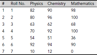
Example 5.2 (Information system)
Table 5.2 shows an information system regarding the scores of seven students in three subjects. The information system consists of seven objects, each corresponding to a student. Here U includes the objects (1, 82, 90, 98), ...., (7, 10, 12, 0) and the set A consists four attributes Roll No., Physics, Chemistry and Mathematics. V (Roll No.) = {1, 2, 3, 4, 5, 6, 7} and V (Physics) = V (Chemistry) = V (Mathematics) = {0, 1, 2, ..., 100}, assuming that the score of a subject is given as whole numbers.
Table 5.2. An information system
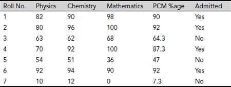
Quite often, an information system includes a special attribute that presents a decision. For example, the information system shown in Table 5.2 may be augmented with a special attribute Admitted as in Table 5.3. This attribute will indicate whether the student concerned is admitted to a certain course on the basis of the marks scored in Physics, Chemistry and Mathematics. Such systems which show the outcome of a classification are known as decision systems. The attribute presenting the decision is called the decision attribute. Values of the decision attribute depend on the combination of the other attribute values.
Example 5.3 (Decision system)
Table 5.3 presents a decision system obtained by augmenting the information system depicted in Table 5.2 by a decision attribute Admitted.
Table 5.3. An information system augmented with a decision attribute
Definition 5.2 (Decision System) A decision system D (U, A, d) is an information system I (U, A) augmented with a special attribute d ∉ A, known as the decision attribute.
The decision system shown in Table 5.3 has the decision attribute Admitted that has binary values ‘Yes’ or ‘No’. These values are based on certain rules which guide the decision. On a closer scrutiny into Table 5.3, this rule maybe identified as If PCM %age is greater than or equal to 87.3 then Admitted = Yes, else Admitted = No.
5.2 INDISCERNIBILITY
Decision systems have the capacity to express knowledge about the underlying information system. However, a decision table may contain redundancies such as indistinguishable states or superfluous attributes. In Table 5.3, the attributes Physics, Chemistry and Mathematics are unnecessary to take decision about admittance so long as the aggregate percentage is available. The decision attributes in decision systems are generated from the conditional attributes. These conditional attributes share common properties as clarified in the subsequent examples. However, before we go on to discuss these issues, we need to review the concept of equivalence relation.
Definition 5.3 (Equivalence Relation) A binary relation R ⊆ A × A is an equivalence relation if it is
(i) |
Reflexive |
(∀ x ∈ A, xRx), |
(ii) |
Symmetric |
(∀ x, y ∈ A, xRy ⇒ yRx), and |
(iii) |
Transitive |
(∀ x, y, z ∈ A, xRy ∧ yRx ⇒ xRz). |
Informally, two objects or cases are equivalent if they share some common properties. Equivalence is however, limited only to those common properties which these elements share.
Example 5.4 (Equivalence relation)
As a rather trivial case, let us consider similarity (~) of triangles. Two triangles ΔABC and ΔPQR are similar (written as ΔABC ~ ΔPQR) if they have the same set of angles, say ∠A = ∠P, ∠B = ∠Q, and ∠C = ∠R. This is an equivalence relation because
- ~ is reflexive (ΔABC ~ ΔABC),
- ~ is symmetric (ΔABC ~ ΔPQR ⇒ ΔPQR ~ Δ ABC), and
- ~ is transitive (ΔABC ~ ΔPQR ∧ ΔPQR ~ Δ KLM ⇒ ΔABC ~ Δ KLM).
Example 5.5 (Equivalence relation)
Let us consider a case of hostel accommodation. Let S be a set of students and R be a relation on S defined as follows : ∀ x, y ∈ S, xRy if and only if x and y are in the same hostel. R is an equivalence relation because
- R is reflexive (A student stays in the same hostel as himself.)
- R is symmetric (If x stays in the same hostel as y, then y stays in the same hostel as x), and
- R is transitive (If x stays in the same hostel as y, and y stays in the same hostel as z, then x stays in the same hostel as z).
Let I be the set of all integers and let R be a relation on I, such that two integers x and y are related, xRy, if and only if x and y are prime to each other. This relation is symmetric but neither reflexive nor transitive. Therefore it is not an equivalence relation.
Example 5.7 (Equivalence Relation)
Let us consider matrix algebra and multipliability of matrices. Two matrices A and B are related if A × B is defined. This relation is neither reflexive, nor symmetric, nor transitive. Hence it is not an equivalence relation.
Definition 5.4 (Equivalence Class) An equivalence class of an element x ∈ U, U being the universe, is the set of all elements y ∈ U such that xRy, i.e., x and y are related. Hence, if E ⊆ U, be an equivalence class, then ∀ a, b ∈ E, aRb holds good.
Example 5.8 (Equivalence Class)
Let U = {0, 1, 2, 3, 4, 5, 6, 7, 8, 9} and ∀ a, b ∈ U, aRb if and only if a MOD 3 = b MOD 3. This relation partitions U into three equivalence classes corresponding to the x MOD 3 = 0, 1, and 2. These equivalence classes are {0, 3, 6, 9}, {1, 4, 7}, and {2, 5, 8} respectively.
Definition 5.5 (Indiscernibility) Let I = (U, A) be an information system where U = {(a1, …, ak)} is the non-empty finite set of k-tuples known as the objects and U = {A1, …, Ak} is a non-empty finite set of attributes. Let P ⊆ A be a subset of the attributes. Then the set of P-indiscernible objects is defined as the set of objects having the same set of attribute values.
The concept of indiscernibility is illustrated in Example 5.9.
Table 5.4. Personnel profiles

Example 5.9 (Indiscernibility)
Consider the profiles of a set of persons as shown Table 5.4. Let P = {Gender, Complexion, Profession} ⊆ A = {Gender, Nationality, Complexion, Mother-tongue, Profession}. From the information system shown in Table 5.4 Catherine and Dipika are P-indiscernible as both are fair complexioned lady journalists. Similarly, Amit and Lee are also P-indiscernible. Hence, INDI (P) = {{Catherine, Dipika}, {Amit, Lee}}. On the other hand, the set of P-indiscernible objects with respect to P = {Gender, Complexion} happens to be INDI (P) = {{Amit, Lee}, {Bao}, {Catherine, Dipika}}.
Example 5.10 (Indiscernibility)
Table 5.5 presents an information system regarding various features of three types of cars, viz., Car A, B and C. Unlike the other tables, the attributes are arranged here in rows while the objects are along the columns.
Table 5.5. Car features
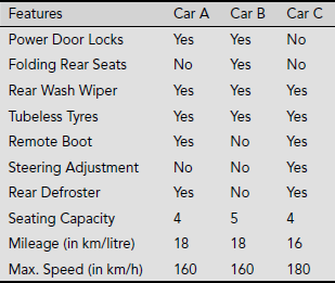
Here, A = {Power Door Locks, Folding Rear Seat, Rear Wash Wiper, Tubeless Tyres, Remote Boot, Steering Adjustment, Rear Defroster, Seating Capacity, Mileage, Max. Speed}, U = {Car A, Car B, Car C}. Let us consider the three subsets of attributes M = {Mileage, Max. Speed}, R = {Rear Wash Wiper, Remote Boot, Rear Defroster} and L = {Power Door Locks, Steering Adjustment}. Then INDI (M) = {{Car A, Car B}, {Car C}}, INDI (R) = {{Car A, Car C}, {Car B}}, INDI (L) = {{Car A, Car B}, {Car C}}.
Indiscernibility is an equivalence relation and an indiscernibility relation partitions the set of objects in an information system into a number of equivalence classes. The set of objects B-indiscernible from x is denoted as [x]B. For example, if B = {Folding Rear Seats, Rear Wash Wiper, Tubeless Tyres, Remote Boot, Rear Defroster}, then [Car A]B = {Car A, Car C}. However, if F = {Power Door Locks, Steering Adjustments, Mileage, Max. Speed}, then [Car A]F = {Car A, Car B}.
5.3 SET APPROXIMATIONS
In a decision system, the indiscernibility equivalence relation partitions the universe U into a number of subsets based on identical values of the outcome attribute. Such partitions are crisp and have clear boundaries demarcating the area of each subset. However, such crisp boundaries might not always be possible. For example consider the decision system presented in Table 5.6. It consists of age and activity information of eight children aged between 10 to 14 months. The outcome attribute ‘Walk’ has the possible values of YES or NO depending on whether the child can walk or not. A closer observation reveals that it is not possible to crisply group the pairs (Age, Can Walk) based on the outcome into YES / NO categories. The problem arises in case of entries 1 and 5 where the ages of the children are same but the outcomes differ. Therefore, it is not possible to decisively infer whether a child can walk or not on the basis of its age information only.
Table 5.6. Child activity information
| # | Age (in months) | Can Walk |
|---|---|---|
1 |
12 |
No |
2 |
14 |
Yes |
3 |
14 |
Yes |
4 |
13 |
Yes |
5 |
12 |
Yes |
6 |
10 |
No |
7 |
10 |
No |
8 |
13 |
Yes |
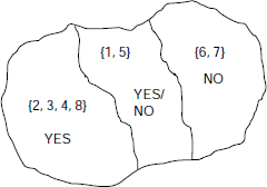
Fig. 5.1. Roughness in a decision system
The situation is depicted in Fig. 5.1. Objects 2, 3, 4 and 8 belong to the class that can be described by the statement ‘If age is 13 or 14 months then the child can walk’. Similarly, objects 6 and 7 define a class corresponding to the rule ‘If age is 10 months then the child can not walk’. However, objects 1 and 5 are on the boundary region in the sense that though both of them correspond to children of age 12 years, their ‘Can Walk’ information is NO in case of object 1 and YES in case of object 5. It is under such circumstances that the concept of rough sets comes into the picture and informally we may say that ‘Sets which consist objects of an information system whose membership cannot be ascertained with certainty or any measure of it are called rough sets. Formally, rough sets are defined in terms of lower and upper approximations. These are described below.
Definition 5.6 (Lower and Upper Approximations) Let I = (U, A) be an information system and B ⊆ A is a subset of attributes and X ⊆ U is a set of objects. Then
The objects that comply with the condition 5.1 and fall in B (X) are classified with certainty as members of set X, while, those objects that comply with 5.2 and therefore belong to ![]() are classified as possible members.
are classified as possible members.
Definition 5.7 (Boundary Region) The set ![]() is called the B-boundary region of X. The B-boundary region of X consists of those objects which we cannot decisively classify as inside or outside the set X on the basis of the knowledge of their values of attributes in B. If a set has a nonempty boundary region, it is said to be a rough set.
is called the B-boundary region of X. The B-boundary region of X consists of those objects which we cannot decisively classify as inside or outside the set X on the basis of the knowledge of their values of attributes in B. If a set has a nonempty boundary region, it is said to be a rough set.
Definition 5.8 (Outside Region) The set ![]() is called the B-outside region of X. The B-outside region of X consists of elements that are classified with certainty as not belonging to X on the basis of knowledge in B.
is called the B-outside region of X. The B-outside region of X consists of elements that are classified with certainty as not belonging to X on the basis of knowledge in B.
Example 5.11 (Set approximations)
With reference to the information system presented in Table 5.6, let W = {y | Can Walk (y) = Yes} = {2, 3, 4, 5, 8}. Now, the set of Age-indiscernible objects of U, IND Age (U) = {{1, 5}, {2, 3}, {4, 8}, {6, 7}}. Hence the sets of the Age-indiscernible objects for various objects are [1] Age = [5] Age = {1, 5}, [2] Age = [3] Age = {2, 3}, [4] Age = [8] Age = {4, 8}, [6] Age = [7] Age = {6, 7}. Thus, assuming B = {Age} we have
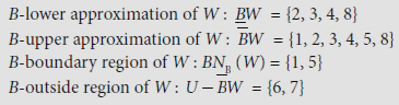
As BNB (W) ={1, 5} ≠ Ø, W is a rough set with respect to knowledge about walking.
5.4 PROPERTIES OF ROUGH SETS
Rough sets, defined as above in terms of the lower and upper approximations, satisfy certain properties. Some of these properties are cited below. These properties are either obvious or easily provable from the definitions presented above.
5.5 ROUGH MEMBERSHIP
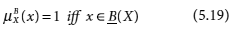
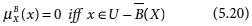
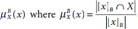
Rough sets are also described with the help of rough membership of individual elements. The membership of an object x to a rough set X with respect to knowledge in B is expressed as ![]() . Rough membership is similar, but not identical, to fuzzy membership. It is defined as
. Rough membership is similar, but not identical, to fuzzy membership. It is defined as
Obviously, rough membership values lie within the range 0 to 1, like fuzzy membership values.
The rough membership function may as well be interpreted as the conditional probability that x belongs to X given B. It is the degree to which x belongs to X in view of information about x expressed by B. The lower and upper approximations, as well as the boundary regions, can be defined in terms of rough membership function.
Example 5.12 (Rough membership)
Let us again consider the information system presented in Table 5.6. W = {y | Can Walk (y) = Yes} = {2, 3, 4, 5, 8} and B = {Age}. In Example 5.11 we have found INDAge(U) = {{1, 5}, {2, 3}, {4, 8}, {6, 7}}, BW = {2, 3, 4, 8}, ![]() , BNB (W) = {1, 5}, and
, BNB (W) = {1, 5}, and ![]() . Moreover, [1]Age = [5]Age = {1, 5}, [2]Age = [3]Age = {2, 3}, [4]Age = [8]Age = {4, 8}, [6]Age = [7]Age = {6, 7}. Now
. Moreover, [1]Age = [5]Age = {1, 5}, [2]Age = [3]Age = {2, 3}, [4]Age = [8]Age = {4, 8}, [6]Age = [7]Age = {6, 7}. Now
Similarly,
The properties listed below are satisfied by rough membership functions. These properties either follow from the definition or are easily provable.
- 0 < μB (x) < 1 iff x ∊ BNB (X) (5.21)


We are now in a position to define rough sets from two different perspectives, the first using approximations and the second using membership functions. Both definitions are given below.
Definition 5.9 (Rough Sets) Given an information system I = (U, A), X ⊆ U and B ⊆ A, roughness of X is defined as follows.
- Set X is rough with respect to B if
- Set X is rough with respect to B if there exist x∈ U such that
Based on the properties of set approximations and the definition of indiscernibility, four basic classes of rough sets are defined. These are mentioned in Table 5.7.
Table 5.7. Categories of vagueness
| # | Category | Condition |
|---|---|---|
1 |
X is roughly B-definable |
|
2 |
X is internally B-definable |
|
3 |
X is externally B-definable |
|
4 |
X is totally B-indefinable |
|
We can further characterize rough sets in terms of the accuracy of approximation, defined as
It is obvious that 0 ≤αB (X) ≤ 1. If αB (X) = 1, the set X is crisp with respect to B, otherwise, if αB (X) < 1, then X is rough with respect to B.
Definition 5.10 (Dependency) Let I = (U, A) be an information system and B1, B2 ∈ A are sets of attributes. B1 is said to be totally dependent on attribute B2 if all values of attribute B1 are uniquely determined by the values in B2. This is denoted as B2 ⇒ B1.
5.6 REDUCTS
An indiscernibility relation partitions the objects of an information system into a set of equivalence classes. However, the entire set of attributes, A, may not be necessary to preserve the indiscernibility among a set of indiscernible objects. In other words, there may exist a subset B ⊆ A, which is sufficient to maintain the classification based on indiscernibility. A minimal set of attributes required to preserve the indiscernibility relation among the objects of an information system is called a reduct.
Definition 5.11 (Reduct) Given an information system I = (U, A), a reduct is a minimal set of attributes B ⊆ A such that INDI (B) = INDI (A).
Definition 5.12 (Minimal Reduct) A Reduct with minimal cardinality is called a minimal reduct.
Table 5.8. Dog breed comparison
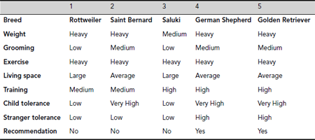
Example 5.13 (Reduct)
Let us consider the information system I = (U, {Weight, Grooming, Exercise, Living Space, Training, Child Tolerance, Stranger Tolerance}, {Recommendation}), concerning comparative study of dog breed, as shown in Table 5.8. For convenience, the attributes are arranged rowwise and the individual objects are presented columnwise.
Here INDI (A) = {{Rottweile r}, {Saint Bernard}, {Saluki}, {German Shepard, Golden Retriever}}. The same equivalence classes are obtained if we consider only two of the attributes B = {Training, Child Tolerance}. However, the classification is different if we remove any of the attributes from the set B = {Training, Child Tolerance}. Therefore, B is a minimal set of attributes. Thus B = {Training, Child Tolerance} is a reduct of the given information system. Moreover, let us consider the set C = {Weight, Grooming, Living Space}. We see that INDI (C) = INDI (B) = INDI (A), however the same set of equivalence classes is obtained for the set C’ = {Weight, Grooming} ⊆ C = {Weight, Grooming, Living Space}. As C is not a minimal set of attributes to maintain the INDI (A) classification, it is not a reduct. Again, the set of attributes D = {Grooming, Living Space} produces the D-indiscernible classes INDI (D) = {{Rottweiler, Saluki}, {Saint Bernard, German Shepard, Golden Retriever}} ≠ INDI (A). Hence D is not a reduct. Moreover, as there is no reduct of size less than 2 for this information system, the set B = {Training, Child Tolerance} is a minimum reduct.
For practical information systems with a large number of attributes, the process of finding a minimum reduct is highly computation intensive. A method based on discernibility matrix is presented below.
Definition 5.13 (Discernibility Matrix) Given an information system I = (U, A) with n objects, the discernibility matrix D is a symmetric n × n matrix where the (i, j)th element dij is given by dij = {a ∈ A| a (xi) ≠ a (xj)}
Each entry of a discernibility matrix is one or more attributes for which the objects xi and xj differ.
Example 5.14 (Discernibility Matrix)
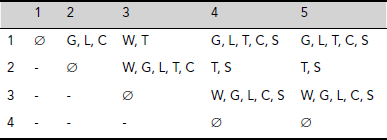
The discernibility matrix for the information system depicted in Table 5.8 on dog breed comparison is shown in Table 5.9. Here d12 = {G, L, C}, which means that object #1 and #2, i.e., the breeds Rottweiler and Saint Bernard differ in the attributes Grooming, Living Space, and Child Tolerance. They match in the rest of the attributes of the information system.
Table 5.9. Discernibility matrix for dog breed information system
Definition 5.14 (Discernibility Function) A discernibility function fI for an information system I = (U, A) is a Boolean function of n Boolean variables a1, a2, ..., an corresponding to the n number of attributes A1, ..., An such that
where dij is the (i, j)th entry of the discernibility matrix.
The set of all prime implicants corresponds to the set of all reducts of I. Hence, our aim is to find the prime implicants of fI.
Example 5.15 (Discernibility Function)
The discernibility function for the discernibility matrix shown in Table 5.9 is given by fI (B, W, G, E, L, T, C, S)
The prime implecants are (G ∧ W ∧ S), (L ∧ W ∧ S), (C∧ W ∧ S), (G ∧ T), (L ∧ T), and (C ∧ T). Each of the sets {G, W, S}, {L, W, S}, {C, W, S}, {G, T}, {L, T}, and {C, T} is a minimal set of attributes that preserves the classification INDI (A). Hence each of them is a reduct. Moreover, each of the sets {G, T}, {L, T}, and {C, T} is a minimal reduct because they are of size 2, and there is no reduct of size smaller than 2 for the present information system.
5.7 APPLICATION
The theory of rough sets is fast emerging as an intelligent tool to tackle vagueness in various application areas. It provides an effective granular approach for handling uncertainties through set approximations. Several software systems have been developed to implement rough set operations and apply them to solve practical problems. Rough set theory is successfully employed in image segmentation, classification of data and data mining in the fields of medicine, telecommunication, and conflict analysis to name a few.
Example 5.16 illustrates the process of rule generation from a given information system / decision system. Subsequently, Example 5.17 presents a case study to show how the concepts of rough set theory can be used for the purpose of data clustering.
Table 5.10. Decision system relating to scholarship information
Example 5.16 (Rule generation)
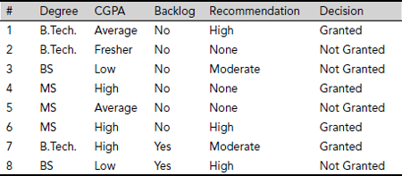
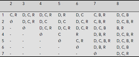
Let us consider a decision system D = (U, {Degree, CGPA, Backlog, Recommendation}, {Decision}) concerning scholarship granting information at an educational institution, as shown in Table 5.10. Table 5.11 presents the corresponding discernity table.
Table 5.11. Discernibility matrix for information system of Table 5.10
The discernibility function obtained from the discernibility table is as follows (using ‘+’ for the logical operator ![]() and ‘·’ for ∧).
and ‘·’ for ∧).
f I (D, C, B, R) =
[(C + R)(D + C + R)(D + C + R)(D + R)(D + C)(C + B + R)(D + C + B)]
[(D + C + R)(D + C)(D + C)(D + C + R)(C + B + R)(D + C + B + R)] .
[(D + C + R)(D + C + R)(D + C + R)(D + C +B)(B + R)].
[(C)(R)(D + B + R)(D + C + B + R)] .
[(C + R)(D + C + B + R)(D + C + B + R)].
[(D + B + R)(D + C + B)]
[(D + C + R)] = (C) · (R)
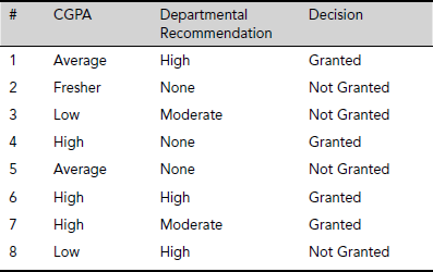
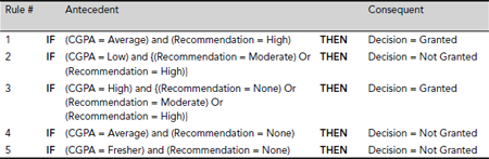
Hence the system has a unique minimum reduct {CGPA, Recommendation}. The sample space after attribute reduction is shown in Table 5.12. The rules extracted using the minimal reduct obtained above are given in Table 5.13.
Table 5.12. Sample space after attribute reduction
Example 5.17 (Data Clustering)
In this example, we consider an animal world dataset based on an example cited by T. Herawan, et. al. in the paper entitled ‘Rough Set Approach for Categorical Data Clustering,’ in International Journal of Database Theory and Application, Vol. 3, No.1. March 2010. We illustrate the process of data clustering using the concepts of rough set theory.
Table 5.14. Animal world dataset
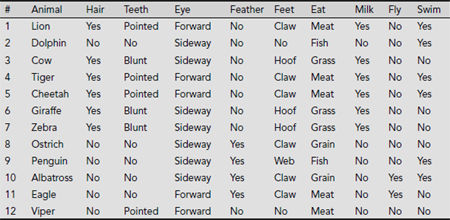
Table 5.14 presents data related to twelve animals, viz., Lion, Dolphin, Cow, Tiger, Cheetah, Giraffe, Zebra, Ostrich, Penguin, Albatross, Eagle, and Viper. The attributes are Hair (whether the animal has hair or not), Teeth, Eye (whether the eyes are directed forward or sideways), Feather, Feet (the options are clawed, hoofed, webbed, or no feet), Eat (i.e, eating habit, options are meat, grass, fish, grain), Milk, Fly, and Swim. The sets of attribute values are, VHair = {Yes, No}, VTeeth = {Pointed, Blunt, No}, VEye = {Forward, Sideway}, VFeather = {Yes, No}, VFeet = {Claw, Hoof, Web, No}, VEat = {Meat, Grass, Grain, Fish}, VMilk = {Yes, No}, VFly = {Yes, No}, VSwim = {Yes, No}.
The partitions using singleton attributes are as given below.
- X (Hair = yes) = {1, 3, 4, 5, 6, 7}, X (Hair = no) = {2, 8, 9, 10, 11, 12}.
∴INDI (Hair) = {{1, 3, 4, 5, 6, 7}, {2, 8, 9, 10, 11, 12}}.
- X (Teeth = pointed) = {1, 4, 5, 12}, X (Teeth = Blunt) = {3, 6, 7}, X (Teeth = no) = {2, 8, 9, 10, 11}.
∴INDI (Teeth) = {{1, 4, 5, 12}, {3, 6, 7}, {2, 8, 9, 10, 11}}.
- X (Eye = Forward) = {1, 4, 5, 11, 12}, X (Eye = Sideway) = {2, 3, 6, 7, 8, 9, 10}.
∴INDI (Eye) = {{1, 4, 5, 11, 12}, {2, 3, 6, 7, 8, 9, 10}}.
- X (Feather = yes) = {8, 9, 10, 11}, X (Feather = no) = {1, 2, 3, 4, 5, 6, 7, 12}.
∴INDI (Feather) = {{8, 9, 10, 11}, {1, 2, 3, 4, 5, 6, 7, 12}}.
- X (Feet = claw) = {1, 4, 5, 8, 10, 11}, X (Feet = hoof) = {3, 6, 7}, X (Feet = Web) = {9}, X (Feet = No) = {2, 12}.
∴INDI (Feet) = {{1, 4, 5, 8, 10, 11}, {3, 6, 7}, {9}, {2, 12}}.
- X (Eat = Meat) = {1, 4, 5, 11, 12}, X (Eat = Grass) = {3, 6, 7}, X (Eat = Grain) = {8, 10}, X (Eat = Fish) = {2, 9}.
∴INDI (Eat) = {{1, 4, 5, 11, 12}, {3, 6, 7}, {8, 10}, {2, 9}}.
- X (Milk = Yes) = {1, 3, 4, 5, 6, 7}, X (Milk = No) = {2, 8, 9, 10, 11, 12}.
∴INDI (Milk) = {{1, 3, 4, 5, 6, 7}, {2, 8, 9, 10, 11, 12}}.
- X (Fly = Yes) = {10, 11}, X (Fly = no) = {1, 2, 3, 4, 5, 6, 7, 8, 9, 12}.
∴INDI (Fly) = {{10, 11}, {1, 2, 3, 4, 5, 6, 7, 8, 9, 12}}.
- X (Swim = Yes) = {1, 2, 4, 5, 9, 10}, X (Swim = No) = {3, 6, 7, ,8, 11, 12}.
∴INDI (Swim) = {{1, 2, 4, 5, 9, 10}, {3, 6, 7, 8, 11, 12}}.
Now, let us focus on the dependency between the attributes Teeth and Hair. We already have INDI (Teeth) = {{1, 4, 5, 12}, {3, 6, 7}, {2, 8, 9, 10, 11}} and INDI (Hair) = {{1, 3, 4, 5, 6, 7}, {2, 8, 9, 10, 11, 12}}. Since {3, 6, 7} ⊆ {1, 3, 4, 5, 6, 7} and {2, 8, 9, 10, 11} ⊆ {2, 8, 9, 10, 11, 12}, but {1, 4, 5, 12} ![]() {1, 3, 4, 5, 6, 7} and {1, 4, 5, 12}
{1, 3, 4, 5, 6, 7} and {1, 4, 5, 12} ![]() {2, 8, 9, 10, 11, 12}, the attribute dependency of Hair on Teeth is computed as follows
{2, 8, 9, 10, 11, 12}, the attribute dependency of Hair on Teeth is computed as follows
This implies that the attribute Hair is partially dependent on the attribute Teeth. The other attribute dependencies for Hair are found similarly.
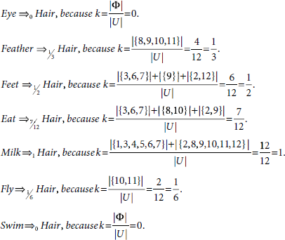
It is found from these calculations that there is complete dependency between the attributes Milk and Hair. Therefore the animal world depicted in the information system Table 5.14 can be partitioned into two clusters on the basis of these two attributes. The resultant clusters are shown in Fig. 5.2.
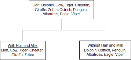
Fig. 5.2. Clusters in the animal world
CHAPTER SUMMARY
The main points of the topics discussed in this chapter are summarized below.
- Theory of rough sets provides a formalism to tackle vagueness in real life relating to information systems.
- An information system is a set of data presented in structured, tabular form. It consists of a universe of objects and a number of attributes. Each object is an ordered n-tuple. The ith element of an object is a possible value of the ith attribute.
- A decision system is an information system with a special attribute called the decision attribute.
- Two objects of an information system are said to be P-indiscernible, where P is a set of attributes of the system, if they have the same set of values of the attributes of P. The P-indiscernibility is an equivalence relation.
- Given an information system I = (U, A), a set of objects X ⊆ U and a set of attributes B ⊆ A, roughness, or otherwise, of X with respect to knowledge in B is defined in terms of the sets B-lower approximation of X and B-upper approximation of X. The B-lower approximation of X is the set of objects that are certainly in X. On the other hand, the set of objects that are possibly in X constitute the B-upper approximation of X. The set X is said to be rough with respect to our knowledge in B if the difference between the B-upper approximation of X and B-lower approximation of X is non-empty.
- The membership of an object x to a rough set X with respect to knowledge in B is expressed as
 . Like fuzzy membership, rough membership values lie within the range 0 to 1.
 - A minimal set of attributes that preserves the indiscernibility relation among the objects of an information system is called a reduct. A minimal reduct is a reduct with minimal size among all reducts.
- A discernibility matrix contains information about pairs of discernibile objects and the attributes in which they differ. A discernibility function presents the same information as a Boolean function in the form of conjunction of disjunctions. The discernibility matrix and the discernibility function are used to find the reducts as well as the minimal reducts of an information system.
- The theory of rough set is applied to extract hidden rules underlying an information system. It is also used for data clustering and data mining applications.
SOLVED PROBLEMS
Problem 5.1 (Set approximations and rough membership) Table 5.14 presents a decision system for a number of individuals seeking loan from a bank and the bank’s decision in this regard. The conditional attributes are Gender, Age, Income, Car (indicating whether the applicant owns a car or not), Defaulter (whether the applicant is a defaulter in paying of a previous loan) and their valid attribute values are {Male, Female}, {Middle-aged, Young-adult, Aged}, {High, Medium, Low}, {Yes, No}, and {Yes, No} respectively. The decision attribute is Loan Granted with value set {Yes, No}.
Let B = {Age, Income, Car} ⊂ A = {Gender, Age, Income, Car, Defaulter} be a set of attributes. Then
- Compute INDB (I)
- If X = {x ∈ U | Loan Granted (x) = Yes} then compute B-lower and B-upper approximations of X and determine if X is rough in terms of knowledge in B.
- Calculate
 for each x ∈ U.
Table 5.14. Loan applicants’ data set
Solution 5.1 The computations are shown below.
- INDB(I) = {{1, 11}, {2}, {3, 8}, {4, 12}, {5}, {6}, {7}, {9, 10}}
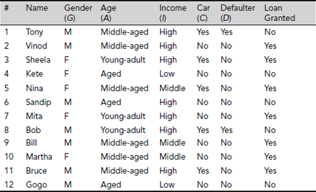
- X = {x ∈ U | Loan Granted (x) = Yes} = {2, 3, 5, 7, 9, 10, 11}
B (X) = {2, 5, 7, 9, 10},
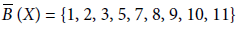 and
andBNB (X) = {1, 8} ≠ ϕ.
∴ X is rough with respect to knowledge of the attributes {Age, Income, Car} (Fig. 5.3).
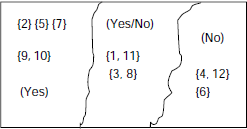
Fig. 5.3 Set approximations
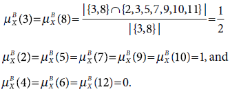
- Computations of the rough membership values for individual elements are shown below.
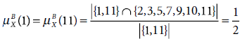
Similarly,
Problem 5.2 (Minimum reduct) We know that the discernibility matrix is constructed to find the reducts of an information system, and thereby the minimal reduct. Each cell of a discernibility matrix correspond to a pair of objects. It contains the attributes in which the pair of objects differ. The discernibility function is a conjunction of terms where each term is constituted from the entries of the discernibility matrix. A term is a disjunction of attributes in a cell of the discernibility matrix.
Propose a technique to simplify the discernibility matrix, or discernibility function, so that the set of reducts and thereby the minimal reducts of the system could be found efficiently. Apply this technique to the information system depicted in Table 5.14 and find it’s minimal reduct.
Solution 5.2 The discernibility function is a conjunction of disjunctions. This function can be simplified by repeated application of the boolean identy
The technique consists of identifying a pair of non-empty cells, say α and β such that all attributes in α are contained in β. We can ignore the set of attributes in β on the basis of the identity 5.27. This way the ‘dependent’ cells are eliminated resulting in a reduced discernibility matrix. The discernibility function is constructed from the reduced matrix and is transformed to a disjunction of conjunction, i.e., sum of products, form. The entire procedure is presented in Procedure Find-Min-Reduct (U, A), shown as Fig. 5.4.
Execution of Procedure Find-Min-Reduct (U, A) for the given information system is described below.
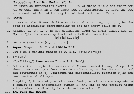
Fig. 5.4 Procedure Find-Min-Reduct (U, A)
Step 1. |
Construct the discernibility matrix D of I. Let c1, c2, , cr be the sets of attributes corresponding to the non-empty cells of D. |
|
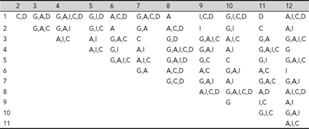
We construct the discernibility matrix for the given information system as shown in Table 5.15. The sets of attributes are {C, D}, {G, A, D}, {G, A, I, C, D}, {G, I, D}, …, {A, I, C}. There are 66 such sets altogether. |
Arrange c1, c2, , cr in non-decreasing order of their sizes. Let C1, C2, , Cr be the rearranged sets of attributes such that |C1| ≤ |C2| ≤ ≤ |Cr|. | |
|
The arrangement is : {A}, {D},{A}, {I}, {C}, {C}, {G}, {C}, {I}, {G}, {C, D}, {G, A}, …, {G, A, I, C, D}. |
Table 5.15. Discernibility matrix
Step 3-7. |
Let T = {} and S = {C1, C2, , Cr} |
Repeat While S ≠ ϕ
Let c be a minimal member of S, i.e., |c| ≤ |Ci| ∀ Ci ∈ S |
|
|
T = T ∪ {c} |
|
∀Ci ∈ S, If c ⊆ Ci, Then remove Ci from S, S = S − {Ci} |
|
All sets of attributes except {A}, {D}, {I}, {C}, {G} are removed in the process described above. Hence, T ={{A}, {D}, {I}, {C}, {G}}. |
Step 8. |
Let t1, t2, , tk be the members of T constructed through Steps 3-7 above. For each ti ∈ T form a Boolean clause Ti as the disjunction of the attributes in ti. Construct the discernibility function fD as the conjunction of all Ti′ s. |
|
Here the discernibility function is fI (G, A, I, C, D) = G ∧ A ∧ I ∧ C ∧ D. |
|
Step 9. |
Simplify fD to sum-of-products form. Each product term corresponds to a reduct of the information system I. Any one of the product terms with minimal cardinality is a minimal reduct of I. |
|
In the present case the discernibility function fI (G, A, I, C, D) = G ∧ A ∧ I ∧ C ∧ D contains a single product term and is already in simplified form. Therefore, the minimum reduct for the given information system is unique and consists of all the attributes A = {Gender, Age, Income, Car, Defaulter}. |
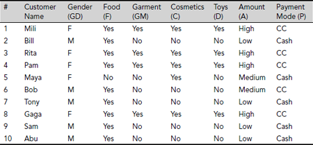
Problem 5.3 (Minimum reduct) Table 5.16 presents data related to the shopping habits of a number of customers to a shopping mall. Four kinds of items, viz., Food (F), Garment (GM), Cosmetics (C), and Toys (T) are considered. If a customer buys a certain kind of item, the corresponding entry in the table is Yes, otherwise No. The attribute Amount (A) express the amount paid by the customer which is either High, or Medium, or Low. There are two modes of payment (P), Cash and Credit Card (CC). Find the reducts of the information system presented in Table 5.16 as well as the minimal reducts from the set of reducts obtained. Also, extract the rules on the basis of one of the minimal reducts and assuming P to be the decision attribute.
Table 5.16. Shopping habit data set
Solution 5.3 The step-by-step process for finding the reducts and the minimal reducts is given below.
Step 1. |
Construct the discernibility matrix D of I. Let c1, c2, …, cr be the sets of attributes corresponding to the non-empty cells of D. |
|
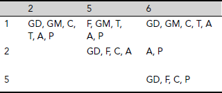
The discernibility matrix constructed is shown in Table 5.17. The blank cells indicate the indiscernible pairs of objects. For example, cell (1, 3) is blank, as the objects 1 and 3 are indescernible. Similarly, null entries at cells (1, 4) and (1, 8) indicate indiscernibility of the objects 1, 4, and 8. As indiscernibility is an equivalence relation, we find that the set {1, 3, 4, 8} forms a class of indiscernible objects. Table 5.17 reveals that indiscernible classes are {1, 3, 4, 8}, {2, 7, 9, 10}, {5}, and {6}. In order to further simplify the process of finding the reducts of the given information system, we reduce the discernibility matrix by taking one object from each of the equivalence classes. The reduced discernibility matrix is shown in Table 5.18. The objects 1, 2, 5 and 6 are considered as representatives of the classes {1, 3, 4, 8}, {2, 7, 9, 10}, {5}, and {6} respectively. |
|
Step 2. |
Arrange c1, c2, , cr in non-decreasing order of their sizes. Let C1, C2, , Cr be the rearranged sets of attributes such that |C1| ≤ |C2| ≤ ≤ |Cr|. |
|
The arrangement is : {A, P}, {GD, F, C, A}, {GD, F, C, P}, {F, GM, T, A, P}, {GD, GM, C, T, A}, {GD, GM, C, T, A, P}. |
Table 5.17. Discernibility matrix for shopping habit data set
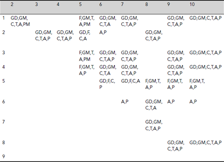
Table 5.18. The reduced discernibility matrix
Step 3-7. |
Let T = {} and S = {C1, C2, , Cr} |
|
Repeat While S ≠ ϕ |
|
Let c be a minimal member of S, i.e., |c|≤|Ci| ∀ Ci ∈ S |
|
|
T = T ∪ {c} |
|
∀ Ci ∈ S, If c ⊆ Ci, Then remove Ci from S, S = S – {Ci} |
|
We find T = {{A, P}, {GD, F, C, A}, {GD, F, C, P}, {GD, GM, C, T, A}}.
|
|
Let t1, t2, , tk be the members of T constructed through Steps 3-7 above. For each ti ∈ T form a Boolean clause Ti as the disjunction of the attributes in ti. Construct the discernibility function fD as the conjunction of all Ti′s. | |
|
The discernibility function is fI (GD, F, GM, C, T, A, P) = (A + P)·(GD + F + C + A)·(GD + F + C + P)·(GD + GM + C + T + A) |
|
Step 9. |
Simplify fD to sum-of-products form. Each product term corresponds to a reduct of the information system I. Any one of the product terms with minimal cardinality is a minimal reduct of I. |
|
After further simplification the discernibility function in sum-of-products form is given by |
|
f I (GD, F, GM, C, T, A, P) = GD·P + A·GD + A·P + A·F + A·C + C·P + F·T·P + F·GM·P = A·(C + F + P + GD) + P·(GD + C + F·T + F·GM) |
|
Therefore, the given information system has eight reducts {GD, P}, {A, GD}, {A, P}, {A, F}, {A, C}, {C, P}, {F, T, P}and {F, GM, P}. Each of the reducts {GD, P}, {A, GD}, {A, P}, {A, F}, {A, C} and {C, P} is a minimal reduct. |
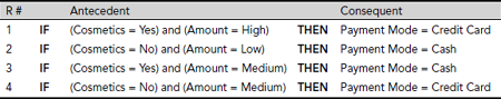
Rules extracted On the basis of the reduct {A, C} and taking P as the decision attribute we get the following rules as shown in Table 5.19.
Table 5.19. Extracted rules
TEST YOUR KNOWLEDGE
5.1 Which of the following is not a part of an information system?
- A non-empty set of objects
- A non-empty set of attributes
- Both (a) and (b)
- None of the above
5.2 Which of the following contains a decision attribute?
- An information system
- A decision system
- Both (a) and (b)
- None of the above
5.3 Two objects of a decision system are said to be indiscernible if
- They have the same decision attribute value
- They have the same conditional attributes value
- Both (a) and (b)
- None of these
5.4 The indiscernibility relation over a given information system is
- Reflexive
- Symmetric
- Transitive
- All of the above
5.5 Let I = (U, A) be an information system and P ⊂ Q ⊂ A and x, y ∈ U be objects of I. Then which of the following statements is true?
- If x and y are P-indiscernible then they are Q-indiscernible
- If x and y are Q-indiscernible then they are P-indiscernible
- The P and Q-indiscernibility of x and y are unrelated
- None of these
5.6 Let I = (U, A) be an information system and B ⊂ A and X ⊂ U. Then which of the following relations holds good for a rough set?


- None of the above
5.7 Let I = (U, A) be an information system and B ⊂ A and X ⊂ U. Then which of the following is defined as the B-boundary region of X?
5.8 Let I = (U, A) be an information system and B ⊂ A and X ⊂ U. Then which of the following is defined as the B-outside region of X?
- U – B(X)


- None of the above
5.9 Let I = (U, A) be an information system and B ⊂ A and X ⊂ U. Then which of the following relations is not valid?
- B(X ∩ Y) = B(X) ∩ B(Y)
- B(X ∪ Y) ⊇ B(X) ∪ B(Y)
- Both (a) and (b)
- None of the above
5.10 Let I = (U, A) be an information system and B ⊂ A and X ⊂ U. Then which of the following relations is not valid?
- Both (a) and (b)
- None of the above
5.11 Which of the following is not true?
- None of the above
5.12 Which of the following is the value of ![]()
- 0
- 1
- Between 0 and 1
- None of the above
5.13 Which of the following relations is true?


- Both (a) and (b)
- None of the above
5.14 If B(X) ≠ Φ and ![]() then
then
- X is totally B-indefinable
- X is externally B-definable
- X is internally B-definable
- X is roughly B-definable
5.15 Let P ⊂ Q ⊂ A be sets of attributes of an information system I = (U, A) such that INDA(P) = INDA(Q). Then which of the following is certainly not true?
- P is not a reduct of U
- Q is not a reduct of U
- Q-P is not a reduct of U
- None of the above
5.16 Let D be the discernity matrix of an information system I = (U, A) with n objects. If the (i, j)th element of D contains an attribute p∈ A, and xi and xj denote the ith and the jth objects of U, then which of the following is true?
- p(xi) = p(xj)
- p(xi) ≠ p(xj)
- p(xi) and p(xj) are not related
- None of the above
5.17 Which of the following helps us to find the minimum reduct of an information system?
- Discernibility Matrix
- Discernibility function
- Both (a) and (b)
- None of the above
5.18 The entries of discernibility matrix consists of
- A set of objects
- A set of attributes
- A rough membership value
- None of the above
5.19 Which of the following is not an application area of the rough set theory?
- Rule extraction
- Data clustering
- Both (a) and (b)
- None of the above
5.20 Which of the following is an appropriate condition for applying rough set theory?
- Non-determinism
- Uncertainty
- Vagueness
- None of the above
Answers
5.1 (d) |
5.2 (b) |
5.3 (b) |
5.4 (d) |
5.5 (b) |
5.6 (a) |
5.7 (b) |
5.8 (b) |
5.9 (d) |
5.10 (d) |
5.11 (d) |
5.12 (b) |
5.13 (c) |
5.14 (a) |
5.15 (b) |
5.16 (b) |
5.17 (c) |
5.18 (b) |
5.19 (d) |
5.20 (c) |
EXERCISES
5.1 Prove that indiscernibility is an equivalence relation.
5.2 Prove the following identities for an information system I = (U, A) and B ⊆ A.
5.3 Consider the information system presented in Table 5.14 showing the loan applicants’ data set. We want to investigate if there is any correlation between the attributes {Age, Income} and possession of a car. If B = {Age, Income}, then
- Find INDB (I)
- Let X = {x ∈ U | x (Car) = Yes}. Find if X is rough in terms of knowledge in B.
5.4 Let I = (U, A) be an information system and C ⊆ B ⊆ A. Then prove that ∀x ∈ U, [x]B ⊆ [x]C.
5.5 Consider the information system presented in Table 5.16 on the shopping habit of a number of customers. As shown in solved problem no. 3, {A, GD} is a minimal reduct of the system. Find the rules underlying the system on the basis of the reduct {A, GD} and taking P as the decision attribute.
5.6 Table 5.8 present an information system on Dog Breed Comparison. Compute the attribute dependencies X → Grooming for all attributes X other than Grooming, i.e. X ∈ {Weight, Exercise, Living Space, Training, Child Tolerance, Stranger Tolerance}.
Is it possible to partition the cited dog breeds into clusters on the basis of these attribute dependencies? If yes, then show the clusters with the help of a tree structure.
Can you further partition the clusters thus formed into sub-clusters on the basis of knowledge of other attributes?
Do you identify any other attribute dependency on the basis of which the given dog breeds could be partitioned into yet another set of clusters?
5.7 The information system on the shopping habits of a number of customers is given in Table 5.16. Cluster the objects on the basis of the attribute dependencies X → Toys, X being any of the attributes Gender (GD), Food (F), Garment (GM), Cosmetics (C), and modes of payment (P)
5.8 The Solved Problem No. 5.2 proposes a technique to compute the minimal reducts of a given information system. However, there are other methods to find the minimal reducts. Can you devise your own method to solve the problem?
BIBLIOGRAPHY AND HISTORICAL NOTES
After proposal and initiation of rough sets in 1981-1982, there were a few interesting works on rough set theory by Pawlak himself, Iwinski, Banerjee and so on. In 1991, Pawlak threw some light on the utility of rough sets. Next year Skowron and Rauszer published their works on intelligent decision support using the concept of discernibility matrices. By 1992, Rough Set Theory had gained much ground and as suggested from the compilation ‘Intelligent Decision Support - Handbook of Applications and Advances of the Rough Sets Theory,’ significant work were being carried out in the field of intelligent decision support systems using rough sets. In 1994, Pawlak and Andrez Skowron proposed an extension through rough membership functions. In 1997, Pawlak published on the applicability of rough set theory on data analysis and in the same year E. Orlowska applied the principles on incomplete information systems. First notable application of rough sets on data mining was published by T.Y. Lin and N.Cercone where they dealt with the analysis of imperfect data. Thereafter, a number of applications have come up and rough sets have been used in various areas including data mining and knowledge discovery, pattern classification, incomplete information systems, fault diagnosis, software safety analysis etc. to name a few. Rough sets have also been used in pairs with other soft computing techniques giving birth to such hybrid systems as rough-fuzzy, rough-neural and rough-GA systems. A few important references in this area are given below.
Banerjee, M. and Chakraborty, M. K. (1987). Rough algebra. Bulletin of the Polish Academy of Sciences, Mathematics, 41, 293–287.
Iwinski, T. B. (1987). Algebraic approach to rough sets. Bulletin of the Polish Academy of Sciences, Mathematics, 35, 673–683.
Iwinski, T. B. (1988). Rough orders and rough concepts. Bulletin of the Polish Academy of Sciences, Mathematics, 36, 187–192.
Lin, T.Y. and Cercone, N. (1997). Rough Sets and Data Mining – Analysis of Imperfect Data. Boston: Kluwer Academic Publishers.
Orlowska, E. (1997). Incomplete Information: Rough Set Analysis. Physica-Verlag, Heidelberg.
Pawlak, Z. (1981). Information Systems, Theoretical Foundations. Information Systems, 6, 205-218.
Pawlak, Z. (1982). Rough sets. International Journal of Computer and Information Sciences, 11, 341–356.
Pawlak, Z. (1984). Rough classification. International Journal of Man-Machine Studies, 20, 469–483.
Pawlak, Z., Wong, S. K. M., and Ziarko, W. (1988). Rough sets: Probabilistic versus deterministic approach. International Journal of Man-Machine Studies, 29, 81–95.
Pawlak, Z. (1991). Rough sets: Theoretical aspects of reasoning with data. Kluwer Academic Publishers, Boston.
Pawlak, Z. and Skowron, A. (1994). Rough membership functions. In ‘dvances in the Dempster--Schafer Theory of Evidence,’ R. R., Fedrizzi, M., and Kacprzyk, J. (eds.), New York: Wiley, 251-271.
Pawlak, Z. (1997). Rough Sets: Theoretical Aspects of Reasoning about Data. Dordrecht: Kluwer.
Skowron, A. and Rauszer, C. (1992). The discernibility matrices and functions in information systems. In Intelligent Decision Support – Handbook of Applications and Advances of the Rough Sets Theory, R. Slowiński (ed.), Dordrecht: Kluwer, 331–362.
Ziarko, W. P. (ed.) (1994). Rough sets, fuzzy sets and knowledge discovery. Springer–Verlag, London.
Ziarko, W. P. (2002). Rough set approaches for discovery of rules and attribute dependencies. In Handbook of Data Mining and Knowledge Discovery, Klösgen, W. and Zytkow, J. M. (ed.), Oxford, 328–339.