
7
Pattern Classifiers
Key Concepts
ADALINE (Adaptive Linear Neuron), Hebb Learning, Hebb Nets, Learning Rate, Least Mean Square, MADALINE (Many Adaptive Linear Neurons), MR-I Algorithm, MR-II Algorithm, Perceptrons, Perceptron Learning, Widrow-Hoff Learning
Chapter Outline
Chapter 6 provides an overview of various aspects of artificial neural nets including their architecture, activation functions, training rules, etc. This chapter presents discussions on certain elementary patterns classifying neural nets. Four kinds of nets, viz., Hebb net, Perceptron, ADALINE, and MADALINE, are included here. Among these, the first three are single layer, single output nets, and the last one, MADALINE, is a single-output net with one hidden layer. White Hebb network and Perceptron are trained by their respective training rules, both ADALINE and MADALINE employ the least mean square (LMS), or delta rule. More general multi-layer networks, especially the feed-forward networks, are dealt with later in a separate chapter.
7.1 HEBB NETS
A single-layer feedforward neural net trained through the Hebb learning rule is known as a Hebb net. The Hebb learning rule is introduced in Chapter 6. Example 6.6 illustrates the training procedure for a Hebb net where a net is trained to implement the logical AND function. The detailed algorithm is presented here as Procedure Hebb-Learning (Fig. 7.1). Fig. 7.2 shows the architecture of the Hebb net.
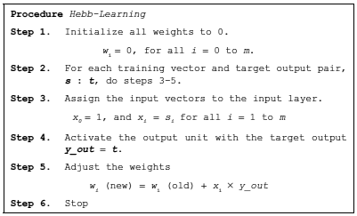
Fig. 7.1 Procedure Hebb-learning
It should be noted that the input unit X0 and the associated weight w0 play the role of the bias. The activation of X0 is always kept at 1. Hence, the expression for adjustment of w0 becomes
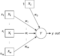
Fig. 7.2. Structure of a Hebb net
Procedure Hebb-Learning requires only one pass through the training set. There are other equivalent methods of applying Hebb learning in different contexts, say, pattern association. Example 6.6 illustrates the training procedure of a Hebb net to realize the AND function. In this example, both the input and output of the function were expressed in bipolar form. Example 7.1 illustrates the limitation of binary representation of data for training a neural net through Hebb learning. Example 7.2 shows that Hebb net may not learn a classification task even if the patterns concerned are linearly separable.
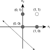
Fig. 7.3. Decision line of Hebb net to realize the AND function when both the input and the output are expressed in binary form
Example 7.1 (Disadvantage of input data in binary form)
In this example, we apply the Hebb learning rule to train a neural net for the AND function with binary inputs. Can the net learn the designated task? We will observe and draw appropriate conclusions from our observation.
Two cases need to be considered. First, the target output is presented in binary, then, in bipolar. The input is in binary form in both cases.
Table 7.1 shows the details of the computation when both the input patterns and the target outputs are presented in binary from. We see that as the target output is 0 for the first three patterns, and as the adjustments Δwi = xi × y_out = xi × 0 = 0, no learning takes place. The final set of weights is (w0, w1, w2) = (1, 1, 1). It can be easily verified that this net fails to classify the patterns (x1, x2) = (0, 0), (0, 1), or (1, 0). Fig. 7.3 shows the decision line for this net. We assume the activation function:
This shows that a Hebb net fails to learn the AND function if both the inputs and the target outputs are expressed in binary. What happens when the output is in bipolar form?
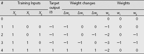
Table 7.2 shows the details of the training process when the output is expressed in bipolar form. As the 0s in the column for 'Target output (t)' are replaced by −1, learning takes place for all training pairs from (0, 0) : (−1) to (1, 1) : (1). The final set of weights are w0 = −2, w1 = 0, w2 = 0. Therefore, the activation of the net is permanently at −1, irrespective of input pattern. It is obvious that though this net classifies the patterns (0, 0), (0, 1), (1, 0) correctly, it is unable to do so for the pattern (1, 1).
Table 7.1 Hebb learning of AND function with Binary Target Output
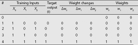
Table 7.2 Hebb learning for AND function (binary input and bipolar output)
The foregoing discussion shows that if the training patterns and the target outputs are presented in binary form, there is no guarantee that a Hebb net may learn the corresponding classification task.
Example 7.2 (Limitation of Hebb net)
This example shows, with the help of a suitable problem instance, that a Hebb net may not be able learn to classify a set of patterns even though they are linearly separable.
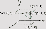
Fig. 7.4. A linearly separable set of points that a Hebb net fails to learn to classify
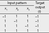
Let us consider four points a (0, 1, 1), b (1, 0, 1), c (1, 1, 0) and d (1, 1, 1) and the corresponding outputs as 0, 0, 0, and 1, respectively. Fig. 7.4 shows these patterns on a 3-dimensional space, and Table 7.3 and Table 7.4 present the training sets expressed in binary and bipolar forms.
Table 7.3. Training pairs in binary form
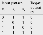
Table 7.4. Training pairs in bipolar form
It is obvious from Fig. 7.4 that the given set of patterns is linearly separable. Any plane that cuts the cube diagonally to isolate the point d (1, 1, 1) from the rest of the three points serves the purpose. In Fig. 7.4, the triangle around the point d represents such a plane. If we present the inputs and the outputs in bipolar form, then a single layer single output net with the interconnection weights w0 = −2, w1 = 1, w2 = 1, and w3 = 1 can solve the classification problem readily (Fig. 7.5).
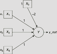
Fig. 7.5. A net to solve the classification problem posed in Table 7.4
Can we make a net learn this, or any other suitable set of weights, through Hebb learning rule so that it acquires the capacity to solve the concerned classification problem? Table 7.5 shows the calculations for such an effort. As the table shows, the weight vector arrived at the end of the process is (w0, w1, w2, w3) = (−2, 0, 0, 0). Now, this set of weights fails to distinguish the pattern (1, 1, 1) from the rest. Hence, the resultant net has not learnt to solve this classification problem.
Table 7.5. Hebb training of classification problem posed in Table 7.4
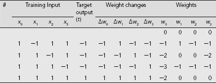
As this network cannot distinguish (1, 1, 1) from the rest, it fails to learn to classify the given patterns even though they are linearly separable.
Hebb net is one of the earliest neural net meant for classification tasks. However, it has very limited capacity. A more powerful ANN is the famous perceptrons. These are discussed in the next section.
7.2 PERCEPTRONS
An overview of perceptrons including their structure, learning rule, etc., is provided in Chapter 6. This section presents the detailed learning algorithm and an example to illustrate the superiority of the perceptron learning rule over the Hebb learning rule. Perceptron learning process is presented as Procedure Perceptron Learning (Fig. 7.6). The notable points regarding Procedure Perceptron-Learning are given below:
- The input vectors are allowed to be either binary or bipolar. However, the outputs must be in bipolar form.
- The bias w0 is adjustable but the threshold θ used in the activation function is fixed.
- Learning takes place only when the computed output does not match the target output. Moreover, as Δ wi = η × t × xi the weight adjustment is 0 if xi = 0. Hence, no learning takes place if either the input is 0, or the computed output matches the target output. Consequently, as training proceeds, more and more training patterns yield correct results and less learning is required by the net.
- The threshold θ of the activation function may be interpreted as a separating band of width 2θ between the region of positive response and negative response. The band itself is ‘undecided’ in the sense that if the net input falls within the range [−θ, θ], the activation is neither positive, nor negative. Moreover, changing the value of θ would change the width of the undecided region, along with the position of the separating lines. Therefore, for Perceptrons, the bias and the threshold are no longer interchangeable.
- The band separating the regions of positive response from that of the negative response is defined by the pair of lines
w0x0 + w1x1 + w2x2 = θw0x0 + w1x1 + w2x2 = −θ (7.2)
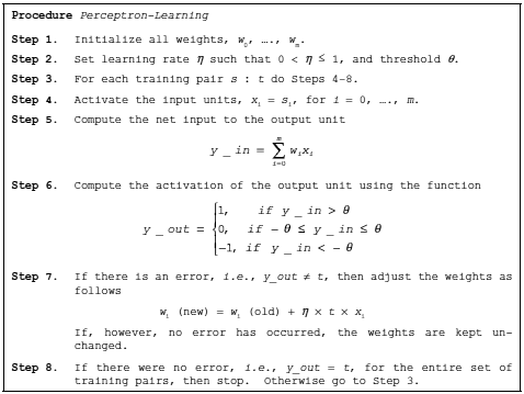
Fig. 7.6. Procedure perceptron learning
Example 7.3 (Power of the perceptron learning rule)
This example intends to show that the perceptron learning rule is more powerful than the Hebb learning rule.
Let us consider the classification problem mentioned in Example 7.2. We have seen that the Hebb learning rule is not powerful enough to train a neural net to realize this classification task even though the concerned patterns are linearly separable. Is it possible to achieve this ability through the perceptron learning rule?
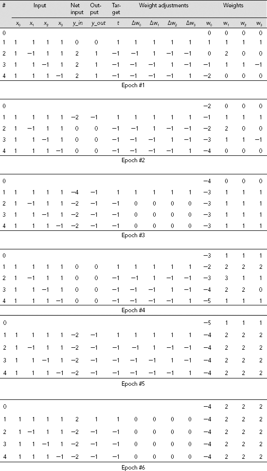
Table 7.6 shows the details of perceptron learning process of the function presented in Table 7.4. For the sake of simplicity, the initial weights are all kept at 0 and the learning rate is set to η = 1. Both the inputs and the outputs are presented in bipolar form. It is seen that five epochs of training are required by the perceptron to learn the appropriate interconnection weights. Calculations at the 6th epoch show that the net successfully produces the expected outputs and no weight adjustments are further required. The final set of the interconnection weights are found to be w0 = −4, w1 = w2 = w3 = 2.
Table 7.6. Perceptron learning of function shown in Table 7.4
7.3 ADALINE
The ADALINE (Adaptive Linear Neuron), introduced by Widrow and Hoff in 1960, is a single output unit neural net with several input units. One of the input units acts as the bias and is permanently fixed at 1. An ADALINE is trained with the help of the delta, or LMS (Least Mean Square), or Widrow-Hoff learning rule. The learning process is presented here as Procedure ADALINE-Learning (Fig. 7.7).
The salient features of ADALINE are
- Both the inputs and the outputs are presented in bipolar form.
- The net is trained through the delta, or LMS, or Widrow-Hoff rule. This rule tries to minimize the mean-squared error between activation and the target value.
- ADALINE employs the identity activation function at the output unit during training. This implies that during training y_out = y_in.
- During application the following bipolar step function is used for activation.
- Learning by an ADALINE net is sensitive to the value of the learning rate. A too large learning rate may prevent the learning process to converge. On the other hand, if the learning rate is too low, the learning process is extremely slow. Usually, the learning rate is set on the basis of the inequality .1 ≤ m × η ≤ 1.0, where m is the number of input units.
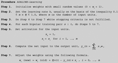
Fig. 7.7. Procedure ADALINE-Learning
Procedure ADALINE-Learning (Fig. 7.7) presents the step by step algorithm for the ADALINE learning process. Learning through the delta rule is illustrated in Chapter 6. Since ADALINE employs the delta learning rule, the training process is practically the same. Example 7.4 illustrates the process of training on ADALINE through the delta rule.
Example 7.4 (ADALINE training for the AND-NOT function)
In this example, we train an ADALINE to realize the AND-NOT function.
The AND-NOT function is presented in Example 6.3. It is a 2-input logic function that produces an output 1 only when x1 = 1, and x2 = 0. For all other input combinations the output is 0. The computations for the learning of an ADALINE to realize the AND-NOT function are shown in Table 7.7. Columns 2, 3, and 4 contain the input patterns expressed in bipolar form. The column x0 stands for the bias which is permanently set to 1. The initial weights are taken as w0 = w1 = w2 = .25, and the learning rate is set to η = .2. As Table 7.8 indicates, the net learns the designated task after the first two epochs.
Table 7.7. ADALINE Learning of AND NOT Function
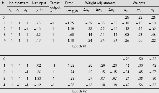
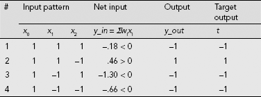
Table 7.8. Performance of the ADALINE after two epochs of learning
7.4 MADALINE
Several ADALINEs arranged in a multilayer net is known as Many ADALINES, or Many Adaptive Linear Neurons, or MADALINE in short. The architecture of a two input, one output, one hidden layer consisting of two hidden MADALINE is shown in Fig. 7.8. MADALINE is computationally more powerful than ADALINE. The enhanced computational power of the MADALINE is due to the hidden ADALINE units. Salient features of MADALINE are mentioned below.
- All units, except the inputs, employ the same activation function as in ADALINE, i.e.,
As mentioned earlier, the enhanced computational power of the MADALINE is due to the hidden ADALINE units. However, existence of the hidden units makes the training process more complicated.
- There are two training algorithms for MADALINE, viz., MR-I and MR-II.
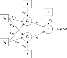
Fig. 7.8. A two input, one output, one hidden layer with two hidden units MADALINE
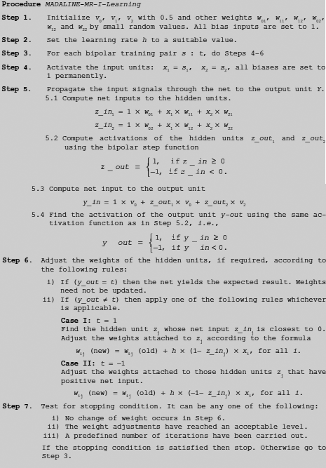
Fig. 7.9. Procedure MADALINE-MRI-Learning
- In MR-I algorithm, only the weights of the hidden units are modified during the training and the weights for the inter-connections from the hidden units to the output unit are kept unaltered. However, in case of MR-II, all weights are adjusted, if required.
The MR-I algorithm (Widrow and Hoff, 1960)
As mentioned earlier, in MR-I training algorithm, the weights associated with the output unit Y, i.e., v0, v1, v2 are fixed and are not altered during the training process. Effectively the output unit Y implements a logical OR operation such that if either of z_out1 or z_out2 is 1 then Y will yield an activation of 1. Hence, v0, v1, v2 are fixed at 0.5. Keeping v0 = v1 = v2 = 0.5 adjustments are done only on w01, w11, w21, w02, w12 and w22 during training. The stepwise training process is given in Procedure MADALINE-MR-I-Learning (Fig. 7.9).
Step 6 of Procedure MADALINE-MRI-Learning is based on two observations:
- The weights should be adjusted only when there is a mismatch between the actual output y_out and the target output t.
- The adjustments of the weights are to be done in a manner so that the possibility of producing the target output is enhanced.
On the basis of these observations, let us analyze the two cases mentioned in Step 6.
Case I: t = 1, and y_out = −1.
As y_out is −1, both z_out1 and z_out2 are −1. To make y_out = 1 = t, we must ensure that at least one of the activations of the hidden units is 1. The unit whose net input is closest to 0 is the suitable unit for this purpose, and the corresponding weights are adjusted as described in Step 6.
Case II: t = −1, and y_out = 1.
In this case, since y_out = 1, at least one of z_out1 and z_out2 must be 1. In order to make y_out = −1 = t, both z_out1 and z_out2 are to be made −1. This implies that all hidden units having positive net inputs are to be adjusted so that these are reduced under the new weights.
Example 7.5 (MADALINE training for the XOR function)
Let us train a MADALINE net through the MR-I algorithm to realize the two-input XOR function.
The architecture of the net is same as shown in Fig. 7.8. The bipolar training set, including the bias input x0 which is permanently fixed at 1 is given in Table 7.9. Table 7.10 presents the randomly chosen initial weights, as well as the learning rate.
The details of the calculations for the first training pair s : t = (1, 1) : −1 of the first epoch of training are described below.
Steps 1–4 are already taken care of. Calculations of Steps (5.1) and (5.2) are given below.
Table 7.9. Bipolar training set for XOR function
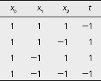
Table 7.10. Initial weights and the fixed learning rate
Step 5.1 |
Compute net inputs z_in1 and z_in2 to the hidden units z1 and z2. |
Step 5.2 |
Compute activations of the hidden units z_out1 and z_out2 using the bipolar step function.
= 1 × .2 + 1 × .3 + 1 × .2 = .7
z_out1 = 1
z_in2 = 1 × w02 + x1 × w12 + x2 × w22
= 1 × .3 + 1 × .2 + 1 × .1 = .6
∴ z_out2 = 1
|
Step 5.3 |
Compute net inputs y_in to the output units. |
Step 5.4 |
Find the activation of the output unit y-out using the same activation function as in Step 5.2, i.e.,
y_in = 1 × v0 + z_out1 × v1 + z_out2 × v2
= 1 × .5 + 1 × .5 + 1 × .5 = 1.5
∴ y_out = 1
|
Step 6 |
Adjust the weights of the hidden units, if required. |
Since t = −1, y_out = 1 ≠ t. Moreover, since t = −1, CASE II of Step 6 is applicable here. Therefore, we have to update weights on all units that have positive net inputs. Hence in this case we need to update the values of w01, w11, w21 as well as those of w02, w12, w22. The computations for the said adjustments are shown below.
Hence the new set of weights after training with the first training pair (1, 1) : −1 in the first epoch is obtained as
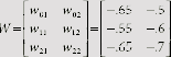
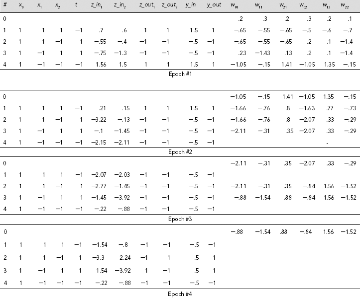
Table 7.11 gives the details of the training process until the MADALINE learns the required function. It is found that four epochs of training are required to arrive at the appropriate weights for realizing the XOR function.
The empty fields in the table indicate no change in the weights. The entries in the Epoch #4 portion of the table show that all the training inputs produce the expected target outputs and consequently, the weights at the beginning of this epoch have remained unchanged. Hence the weights finally arrived at by the MADALINE net are given by
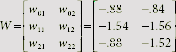
Table 7.11. MADALINE Learning of XOR Function through MR-I algorithm
CHAPTER SUMMARY
An overview of the elementary pattern classifying ANNs, e.g., Hebb nets, Perceptrons, MADALINE and ADALINE have been presented in this chapter. The main points of the foregoing discussion are given below.
- A single-layer feedforward neural net trained through the Hebb learning rule is known as a Hebb net.
- It is possible for a Hebb net not to learn a classification task even if the patterns concerned are linearly separable.
- Perceptrons are more powerful than the Hebb nets. Formula for weight adjustment in perceptron learning is Δ wi = η × t × xi where η is the learning rate.
- The ADALINE (Adaptive Linear Neuron) is a single output unit neural net with several input units. One of the input units acts as the bias and is permanently fixed at 1.
- ADALINE is trained with the help of the delta, or LMS (Least Mean Square), or Widrow-Hoff learning rule.
- Several ADALINEs arranged in a multilayer net is known as Many ADALINES, or Many Adaptive Linear Neurons, or MADALINE in short. MADALINE is computationally more powerful than ADALINE.
- There are two training algorithms for MADALINE, viz., MR-I and MR-II. In MR-I algorithm, only the weights of the hidden units are modified during the training and the weights for the inter-connections from the hidden units to the output unit are kept unaltered. However, in case of MR-II, all weights are adjusted, if required.
SOLVED PROBLEMS
Problem 7.1 (Hebb net to realize OR function) Design a Hebb net to realize the logical OR function.
Solution 7.1 It is observed earlier that a Hebb net may not learn the designated task if the training pairs are presented in binary form. Hence, we first present the truth table of OR function in bipolar form, as given in Table 7.12. Table 7.13 presents the details of the training process. The interconnection weights we finally arrive at are w0 = 2, w1 = 2, and w2 = 2, and the corresponding separating line is given by
Table 7.12 Truth table of OR function in bipolar form
| Input | Output | |
|---|---|---|
| x1 | x2 | x1 OR x2 |
−1 |
−1 |
−1 |
−1 |
1 |
1 |
1 |
−1 |
1 |
1 |
1 |
1 |
Fig. 7.10 shows the location and orientation of this line. The Hebb net, thus, is able to learn the designated OR function.
Table 7.13 Hebb learning of OR function
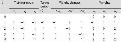
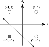
Fig. 7.10. Decision line of Hebb net realizing the OR function
Problem 7.2 (A perceptron and a Hebb net as a traffic controller) A busy town crossing has two signal posts with the usual three-colour light signal system. The post with the rectangular light frame is meant for vehicles plying on the road, while the post with the oval frame is meant for pedestrians trying to cross the road over the zebra. When the traffic light is green, the pedestrian light is red and vice versa while they share a common yellow state. In spite of this arrangement, unruly traffic caused accidents regularly by ignoring the signal. To overcome this problem, the town administration decided to install an automatic gate across the road that will come down across when the traffic light is red and the pedestrian light is green. The state table is as shown in Table 7.14. Design the gate controller with a perceptron, as well as with a Hebb net.
Table 7.14 State table for the traffic controller
Traffic signal |
Pedestrian signal |
Gate |
|---|---|---|
Green |
Red |
Up |
Yellow |
Yellow |
Up |
Red |
Green |
Down |
Solution 7.2 If we decide to design the gate controller based on a perceptron model, we may encode the light colours as described in Table 7.15.
Table 7.15. Traffic controller state table translated to numbers
Traffic signal |
Pedestrian signal |
Gate |
|---|---|---|
2 (Green) |
0 (Red) |
0 (Up) |
1 (Yellow) |
1 (Yellow) |
0 (Up) |
0 (Red) |
2 (Green) |
1 (Down) |
The controller can now be designed as a perceptron on MatLab. The MatLab code for this purpose is shown in Fig. 7.11. Fig. 7.12 depicts the resultant classifier.
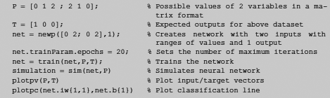
Fig. 7.11. MatLab code for traffic controller perceptron
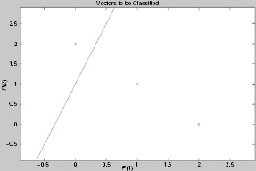
Fig. 7.12. Output plot for traffic controller perceptron
This problem can also be solved using Hebb learning. The corresponding MatLab code is given in Fig. 7.13. Fig. 7.14 (a) and (b) shows the resultant classifier after 20 and 150 epochs of training, respectively. Interestingly, the classification is not satisfactory after only 20 epochs of training. Performance is improved by increasing the number of epochs to 150.
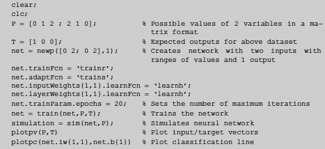
Fig. 7.13. MatLab code for traffic controller Hebb net
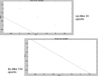
Fig. 7.14. Output plots for Hebbian traffic controller
Problem 7.3 (Classification of two-dimensional patterns with Hebb net) Consider the following patterns to represent the digits 0 and 1 (Fig. 7.15).
Using Matlab design a Hebb net to classify these two input patterns.
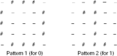
Fig. 7.15. Two 2-dimensional patterns for 0 and 1.
Solution 7.3 For simplicity, let us consider the target class to correspond to the pattern for ‘1’. The patterns not classified as ‘1’ will be treated as ‘0’. Then we convert the patterns into bipolar input vectors by replacing every ‘#’ by ‘1’ and every ‘−’ by ‘−1’ and represent each two dimensional pattern as an input vector by taking the rows and concatenating them one after the other. Fig. 7.16 explains the technique.
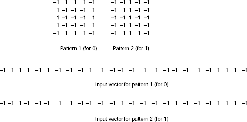
Fig. 7.16. Encoding the input patterns
The MatLab code for the Hebb net to solve the classification problem is given in Fig. 7.17.
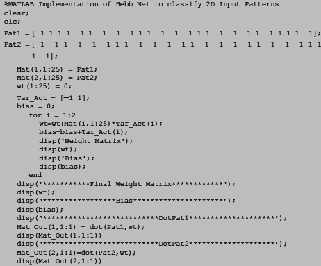
Fig. 7.17. Matlab code for Hebb net of problem 7.3
The output of the training process is given below.
Columns 1 through 22
1 −1 −1 −1 1 −1 1 1 1 −1 −1 1 1 1 −1 −1 1 1 1 −1 1 −1
Columns 23 through 25
−1 −1 1
Bias
−1
Weight Matrix
Columns 1 through 22
0 −2 0 −2 0 −2 2 2 0 −2 −2 0 2 0 −2 −2 0 2 0 −2 0 0
Columns 23 through 25
0 0 0
Bias
0
***********Final Weight Matrix************
Columns 1 through 22
0 −2 0 −2 0 −2 2 2 0 −2 −2 0 2 0 −2 −2 0 2 0 −2 0 0
Columns 23 through 25
0 0 0
*****************Bias*********************
0
*******************DotPat1********************
-24
*******************DotPat1********************
24
TEST YOUR KNOWLEDGE
7.1 How many passes are required by Hebb learning algorithm ?
- One
- Two
- No fixed number of passes
- None of the above
7.2 In which of the following cases Hebb learning does not guarantee that the net will learn the classification task even if it was possible for a Hebb net to learn the task under suitable conditions ?
- The training set is bipolar
- The training set is binary
- Both (a) and (b)
- None of the above
7.3 The statement that a Hebb net may fail to learn a classification task consisting of a linearly separable set of patterns is
- True
- False
- Uncertain
- None of the above
7.4 For Perceptron learning, the bias and the threshold are
- Interchangable
- Not interchangable
- Conditionally interchangable
- None of the above
7.5 Which of the following functions is used for activation of the output unit of the ADALINE during training ?
- Identity
- Binary
- Bipolar step function
- None of the above
7.6 Which of the following functions is used for activation of the output unit of the ADALINE during application ?
- Identity
- Binary
- Bipolar step function
- None of the above
7.7 Which of the following learning rule is used in ADALINE training ?
- Hebb learning
- Perceptron learning
- Delta learning
- None of the above
7.8 Which of the following nets is more powerful than MADALINE ?
- ADALINE
- Hebb
- Both (a) and (b)
- None of the above
7.9 Which of the following is not a pattern classifying net ?
- ADALINE
- MADALINE
- Both (a) and (b)
- None of the above
7.10 Which of the following is a pattern classifying net ?
- ADALINE
- MADALINE
- Both (a) and (b)
- None of the above
Answers
7.1 (a)
7.2 (b)
7.3 (a)
7.4 (b)
7.5 (a)
7.6 (c)
7.7 (c)
7.8 (d)
7.9 (d)
7.10 (c)
EXERCISES
7.1 Design a Hebb net to realize the NAND function.
7.2 Design a Perceptron to realize the NOR function.
7.3 Design an ADALINE to realize the NAND function.
7.4 Design a MADALINE to realize the X-NOR (the complement of XOR) function.
BIBLIOGRAPHY AND HISTORICAL NOTES
The first learning law in the field of artificial neural networks was introduced by Donald Hebb in 1949. Frank Rosenblatt proposed and developed the much celebrated class of ANN called Perceptrons during late fifties and early sixties. ADALINE was proposed by Bernerd Widrow and his student, Mercian Hoff, in 1960. This was closely followed by MADALINE by them. Some milestone works relating to ANN classifiers are here.
Block, H. D. (1962). The Perceptron : A model for brain functioning. Reviews of Modern Physics, Vol. 34, pp. 123–135.
Hebb, D.O. (1961). Distinctive features of learning in the higher animal. In J. F. Delafresnaye (Ed.). Brain Mechanisms and Learning. London: Oxford University Press.
Hebb, D.O. (1949). The Organization of Behavior. New York: Wiley and Sons.
Minsky, M. and Papert, P. (1969). Perceptrons : An Introduction to Computational Geometry. MIT Press.
Rosenblatt, F. (1958). The Perceptron: A Probabilistic Model for Information Storage and Organization in the Brain, Cornell Aeronautical Laboratory. Psychological Review, Vol. 65, No. 6, pp. 386–408.
Rosenblatt, F. (1962). Principles of Neurodynamics. New York: Spartan.
Widrow, B. and Lehr, M. A. (1990). 30 Years of Adaptive Neural Networks : Perceptron, MADALINE and Backpropagation. Proceedings of IEEE, Vol. 78, No. 9, pp. 1415–1442.
Widrow, B. and Stearns, S. D. (1985). Adaptive Signal Processing. Englewood Cliffs, NJ: Prentice-Hall.