
11
Elementary Search Techniques
Key Concepts
8-queen problem, A* algorithm, ‘A’ algorithm, AND-OR graph, AO* algorithm, CNF-satisfiability, Admissibility, Adversarial search, Alpha-beta cut-off, Alpha-beta pruning, Backtracking, Backtracking depth-first search, Best-first search, Bidirectional search, Binary constraint, Blind search, Block world, Book moves, Breadth-first search (BFS), Constraint, Constraint graph, Constraint hypergraph, Constraint propagation, Constraint satisfaction, Control system, Crossword puzzle, Cryptarithmetic puzzle, Degree heuristic, Depth-first iterative deepening, Depth-first search (DFS), Difference-operator-precondition table, Exhaustive search, Final state, Forward checking, Game playing, Game tree, General constraint, General problem solver (GPS), Global database, Goal state, Graph colouring problem, Greedy local search, Heuristic search, Hill climbing, Horizon effect, Informed search, Initial state, Irrevocable control strategy, Least constraining value heuristic, Local optima, Min-conflict heuristic, Minimum remaining value (MRV) heuristic, n-queen problem, Objective function, Operator subgoaling, Plan generation, Plateau, Post-condition, Pre-condition, Problem reduction, Production rules, Production system, Quiescence, Ridge, Secondary search, Start state, State space, State space search, Static evaluation function, Steepest-ascent hill climbing, Traveling salesperson problem, Unary constraint, Uninformed search, Utility function, Valley descending
Chapter Outline
Many intelligent computational processes take the form of state space search, which is at the core of such intelligent systems. This chapter provides a review of these elementary state space search techniques. Evolutionary search techniques e.g. Genetic Algorithms (GAs), Simulated Annealing (SA) etc. are traditionally regarded as soft computational processes. These techniques are applied to tackle highly complex problems. A review of the basic search techniques is necessary for an understanding of the evolutionary search strategies stated above. In this chapter we start with the concept of a state space. Then the basic state space search algorithm is presented and explained. Exhaustive search algorithms, e.g., breadth-first search, depth-first search, depth-first iterative deepening etc., are discussed which is followed by discussions on various heuristic search strategies. The principles underlying such techniques as best-first search, hill climbing, A / A* algorithm, AO* algorithm etc. are explained with appropriate illustrative examples. Features of production systems, an important class of intelligent systems employing state space search at the core, are explained along with examples.
11.1 STATE SPACES
Many intelligent computational processes are modeled as a state space search. The concept of a state space is introduced in this section. Searching through a state space, i.e., state space search, is discussed in the next section.
Let us consider a block world of size three. A block world consists of a number of cubical blocks on a plane surface. The blocks are distinguishable and they may either rest on the table or stacked on it. The arrangement of the blocks constitutes a state of the block world. An arrangement of the blocks can be altered through a set of legal moves. An altered arrangement results in a different state. The size of the block world is given by the number of blocks in it. So, a block world of size three consists of three distinguishable blocks. Let the blocks be marked as X, Y, and Z.
Let the initial stack of the blocks be as shown in Fig. 11.1(a). They are to be rearranged into the goal stack shown in Fig. 11.1(b). The rules to manipulate the block world are:
- Only one block can be moved at a time.
- A block can be moved only if its top is clear, i.e., there is no block over it.
- A block can be placed on the table.
- A block can be placed over another block provided the latter’s top is clear.
We have to find a sequence of legal moves to transform the initial stack of blocks to the goal stack.
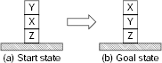
Fig. 11.1. A block manipulation problem.
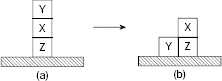
Fig. 11.2. The first move.
The only valid move from the initial arrangement is to lift the topmost block Y and place it on the table to obtain the state in Fig. 11.2(b).
From the state depicted in Fig. 11.2(b) the possible moves are:
- Replace block Y on top of X to return to the previous arrangement, or
- Lift block X and place it on the table, or
- Lift block X and place it on block Y.
Taking this into account, the possibilities regarding the first two moves are shown in Fig. 11.3. Bidirectional arrows indicate that the corresponding changes in the block world are reversible.
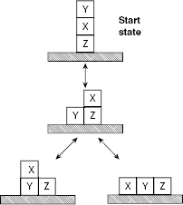
Fig. 11.3. The first two possible moves.
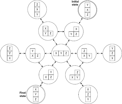
Fig. 11.4. Movements in the block world of size 3.
Similarly, newer block world states are generated by applying appropriate moves. The set of all possible block arrangements and their interrelations are shown in Fig. 11.4. This is a tiny state space of block manipulation problem of size 3.
We may represent each possible state of the block world as a node and express the transition between two states with directed arcs so that the entire set of possible states along with possible transitions among them takes the form of a graph (Fig. 11.5). Finding a solution to the given problem is tantamount to searching for a goal node, (or, a goal state, or final state). The search starts at the start state of the problem, i.e., at the start node. During the search process, newer nodes are generated from the earlier nodes by applying the rules of transformation. The generated nodes are tested for goal, or final, node. Te search stops when a goal is reached, or is found to be unreachable.
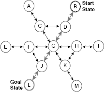
Fig. 11.5. State space of block manipulation problem.
Thus, a state space for a given problem consists of
- A directed graph G(V, E) where each node v ∈ V represents a state, and each edge eij from state vi to vj represents a possible transition from vi to vj. This graph is called the state space of the given problem.
- A designated state s ∈ V referred to as the start state, or start node, of the state space. The search starts from this node.
- A goal condition which must be satisfied to end the search process successfully. It is expected that one or more nodes of the state space will satisfy this condition. Such nodes are called the goal nodes.
The following example illustrates the concept of a state space.
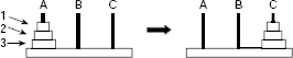
Fig. 11.6. Movements in the block world of size 3
Example 11.1 (State space representation of the Tower of Hanoi problem)
Let us consider the Tower of Hanoi problem for three discs 1, 2, and 3 Fig. (11.6). Discs 1, 2, and 3 are in ascending order of diameter. Initially all the discs are in peg A and the other two pegs B and C are empty. The discs are to be transferred from peg A to peg C so that the final arrangement shown on the right side of Fig. 11.6 is achieved. Disks are transferred from peg to peg subject to the following rules:
- Only one disc may be transferred at a time.
- Under no circumstances a larger disc may be placed over a smaller disc.
- A disc can be picked for movement only if there is no other disc on it.
Let us formulate the problem as a state space search in the following way. The first thing to do is to find a suitable representation of the problem state. We employ here a 3 × 3 matrix to represent a state. Columns 1, 2 and 3 of the matrix correspond to the pegs A, B, and C, respectively. Similarly, the rows are used to indicate the relative positions of the discs within a peg. Thus, the start state and the goal state are expressed as in Fig. 11.7(a) and Fig. 11.7(b).
What about the transitions among the possible states? Initially all discs are in peg A with disc 3 at the bottom and disc 1 at the top. In this situation we can pick disc 1 from the top and put it either in peg B or in peg C (Fig. 11.8). Each of these two states will generate others states (including those already generated) and so on. The partial state space for this problem with one path from the start state to the goal state is shown in Fig. 11.9. The corresponding graph is given in Fig. 11.10. The graph does not show the details of a state and express them simply as nodes. The start node and the goal node are indicated with appropriate tags and the solution path, i.e., the sequence of moves from the start node to the goal node is highlighted.
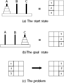
Fig. 11.7. Formulation of Tower of Hanoi problem as a state space search.
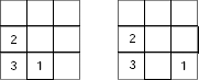
Fig. 11.8. Probable states after the first move.
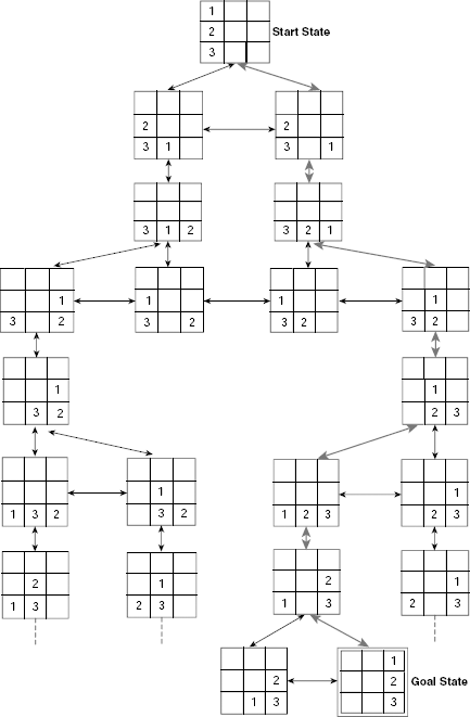
Fig. 11.9. State space of Tower of Hanoi problem with three discs
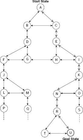
Fig. 11.10. State space of Tower of Hanoi as a graph
Example 11.2 (State space representation of the 8-puzzle)
The 8-puzzle is a combination of eight movable tiles, numbered 1 to 8, set within a 3 × 3 frame. Out of the 3 × 3 = 9 cells eight cells are occupied by the tiles and one remaining cell is empty. At any instant, a tile which is adjacent to the empty cell in the vertical or in horizontal direction, may slide into it. Equivalently, the empty cell can be moved to left, right, up, or down by one cell at a time, depending on its position. The state of the 8-puzzle can be represented with the help of a 3 × 3 matrix where the empty cell is indicated by blank. Given the initial and the goal states of an 8-puzzle as shown in Fig. 11.11, we are to generate the state space and a path from the start state to the goal state in it.
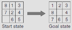
Fig. 11.11. An instance of the 8-puzzle.
Initially the empty cell is at the bottom-left corner. We can move it either upwards or to the right. No other movement is possible from this position. Accordingly, we get two children from the start node. From each of these children, two new states can be generated. If we go on generating newer states and the interconnections among them we get the required state space as shown in Fig. 11.12. Fig. 11.13 hides the details of the individual states and presents the said state space as a directed graph.
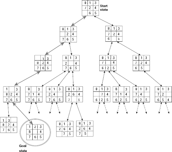
Fig. 11.12. State space of the 8-puzzle.
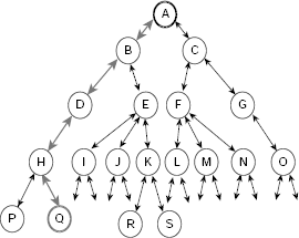
Fig. 11.13. State space of the 8-puzzle as a graph.
11.2 STATE SPACE SEARCH
Once the state space of a given problem is formulated, solving the problem amounts to a search for the goal in it. The basic search process is independent of the problem and has a number of common features as described below.
11.2.1 Basic Graph Search Algorithm
The search starts from the start node which represents the initial state of the problem. As the search proceeds, newer and newer nodes are produced and the search tree grows. The search tree is a subgraph of state space. It consists of the nodes generated during the search. There is a set of transformation rules that map a given node to other nodes. A node is said to be generated when it is obtained as a result of applying some rule on the parent node. A node is said to be expanded when its children are generated. Moreover, there are some conditions to ascertain whether a given node is a goal not. When a node undergoes such a test it is said to be explored.
During the search, two lists are maintained. One for the nodes that have been generated but neither explored, nor expanded. This list is referred to as OPEN. The other list, called CLOSED, contains all nodes that have been generated as well as explored and expanded. While the search process is on, a node from the OPEN list is selected for processing. It is first explored and if found to be a goal node, the search ends successfully. Otherwise, the node is expanded and the newly generated nodes are included into the search tree constructed so far. The process stops successfully when a goal node is reached. It ends unsuccessfully if the list OPEN is found to be empty, indicating that the goal node, if exists, is unreachable from the start node.
A simplified version of the algorithm which focuses on the essential features of state space search is given in Algorithm Basic-State-Space-Search (Fig. 11.14).
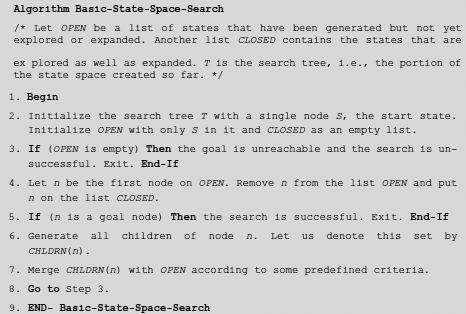
Fig. 11.14. Algorithm basic-state-space-search.
11.2.2 Informed and Uninformed Search
Step 7 of Algorithm Basic-State-Space-Search states that the newly generated nodes are to be merged with the states of the existing OPEN queue. But how this merging should be done is not explained. Actually, the character of a search process depends on the sequence in which the nodes are explored which, in turn, is determined by the way new nodes are merged with the current nodes of OPEN.
All state space searches can be classified into two broad categories, uninformed and informed. They are also referred to as blind search, and heuristic search, respectively. In an uninformed, or blind, search, no knowledge of the problem domain is employed to guide the search for a goal node. On the contrary, an informed, or heuristic, search is guided by some knowledge of the problem domain so that the process may estimate the relative merit of the unexplored nodes with respect to the attainment of a goal node through it. The crucial point is Step 7 of Algorithm Basic-State-Space-Search where the newly generated nodes are merged with the existing OPEN list. The way of merging differentiates between the various kinds of search strategies to be discussed subsequently.
11.3 EXHAUSTIVE SEARCH
An exhaustive search is a kind of blind search that tries to examine each and every node of the state space till a goal is reached or there is no way to proceed. The elementary systematic exhaustive searches are breadth-first search (BFS), depth-first search, depth-first iterative deepening search, and bidirectional search. These are discussed in this section.
11.3.1 Breadth-first Search (BFS)
Breadth-first search explores the search space laterally. It employs a queue to implement OPEN so that while executing Step 7 of Algorithm Basic-State-Space-Search, the newly generated nodes are added at the end of the OPEN. Consequently, the nodes generated earlier are explored earlier in a FIFO fashion. For example, consider the extremely simple and tiny state space depicted in Fig. 11.15. It consists of 13 states A, B, …, M and certain transitions among them. The states G, L and M are the goal states.
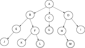
Fig. 11.15. A tiny state space.
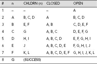
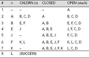
Table 11.1 shows the trace of execution of breadth-first search of the state space given in Fig. 11.15. The search is initialized by putting the start state A on the OPEN queue. At this instant n, CHLDRN (n), and CLOSED are all empty because node A is not yet removed from OPEN and explored. At the 8th row we remove node G, the first node in the OPEN queue at that moment, and examine it. Since G is tested to be a goal node, the search stops here successfully.
Table 11.1. Breadth-first search on Fig. 11.15
Step by step construction of the search tree is shown in Fig. 11.16(a)–(h). Nodes that are generated but not yet explored, or expanded, are highlighted with dotted lines. The unexplored node which is to be explored next is indicated by an arrow. Fig. 11.16(h) shows the final search tree. The dotted arrowed line shows the sequence of nodes visited during the breadth-first search. The search stops as soon as we explore the node G, a goal. It may be noted that except Fig. 11.16(h), node G is shown as an usual node and not a goal node. This is because unless a state is tested it can not be recognized as a goal node even after it has been generated.
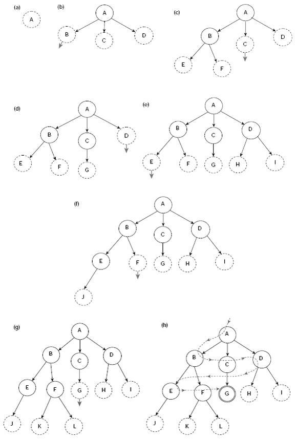
Fig. 11.16. (a)–(h) Breadth-first search (BFS) steps
11.3.2 Depth-first Search (DFS)
While BFS explores the search tree laterally, DFS does so vertically. In DFS, OPEN is implemented as a stack so that the problem states are explored in a LIFO manner. The execution of the depth-first search process can be traced as in case of BFS. As the data structure OPEN should now be a stack rather than a queue the nodes in CHLDRN (n) should be placed in front of OPEN and not at the rear. Table 11.2 depicts the trace of DFS on Fig. 11.15. The construction of the corresponding search tree is shown in Fig. 11.22(a)–(h).
Table 11.2. Depth-first search on Fig. 11.15.
Please note that the DFS tree is different from its BFS counterpart. This is because the nodes explored are different. Moreover, the goals reached are also different. However, in case the state space contains only one goal state then both of these strategies will end with this unique goal. Still, the path from the start node to the goal node would be different for different search strategies.
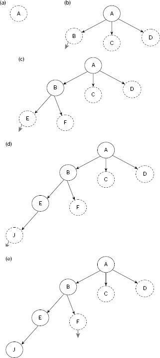
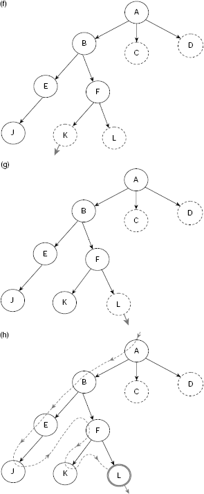
Fig. 11.17. (a)–(h) Depth-first search steps.
11.3.3 Comparison Between BFS and DFS
For a given search problem is it possible to anticipate à-priori which among BFS and DFS would reach a goal earlier. For example, consider the state space of Fig. 11.18(a), which is identical to Fig. 11.15 except that instead of three here we have a single goal node D. If we follow BFS on this graph, we need to explore four nodes to arrive at the goal (Fig. 11.18(b)). The same goal is attained after exploring 10 nodes if we employ DFS (Fig. 11.18(c)). Obviously, the BFS approach is better than DFS in this case. However, the situation is quite the opposite if the goal is located at J instead of D (Fig. 11.19(a)). Here the number of nodes required to explore till we reach the goal using BFS and DFS are 10 and 4, respectively (Fig. 11.19(b) and (c)).
There are some thumb rules to anticipate which, between BFS and DFS, is more efficient for a given problem. Such anticipations are based on some knowledge of the problem domain. For example, if it is known that there are a large number of goal nodes distributed over the entire state space then DFS is probably the right choice. On the other hand, if it contains only one or just a few goal nodes then BFS is perhaps better than DFS.
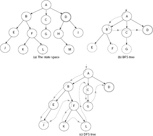
Fig. 11.18. (a)–(c) A state space where BFS is more efficient than DFS.
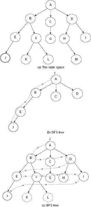
Fig. 11.19. (a)–(c) A state space where DFS is more efficient than BFS.
Both depth-first search and breadth-first search have their own merits and demerits. A comparative study of these two exhaustive search strategies is given in Table 11.3.
Table 11.3. Comparison of DFS and BFS
# |
DFS | BFS |
|---|---|---|
1 |
Requires less memory. |
Requires more memory. |
2 |
May reach a goal at level n+1 without exploring the entire search space till level n. |
All parts of the search space till level n must be explored to reach a goal at level n+1. |
3 |
Likely to reach a solution early if numerous goals exist. |
Likely to reach a solution early even if few goals exist. |
4 |
Susceptible to get stuck in an unfruitful path for a very long time while exploring a path deep into the state space. |
Not susceptible to get stuck in a blind ally. |
5 |
Does not guarantee to offer a minimal-length path from the start state to a goal node. Hence, DFS is not admissible. |
Guarantees to find the minimal-length path from the start node to a goal node. Therefore, BFS is admissible. |
If b is the highest number of successors obtained by expanding a node in the state space, then the time complexity of BFS is O(bd), where d is the depth of the search tree, i.e., the length of the solution path. This can be easily obtained by considering the fact that the most significant computation during the search process is the expansion of a leaf node. The number of nodes generated till depth d is b + b2 + … + bd, which is O(bd). The space complexity is also O(bd) because all nodes at level d must be kept in memory in order to generate the nodes at level d + 1. Hence, BFS is quite expensive in terms of space and time requirements. The time complexity of DFS is also O(bd), same as that of BFS. However, DFS is more efficient in terms of space utilization having space complexity O(b). This is because only the nodes belonging to the path from the start node to the current node are to be stored in case of DFS.
The main problem with DFS is that unless we set a cutoff depth and compel the search to backtrack when the current path exceeds the cutoff, it may not find a goal at all. Setting the cutoff depth is also a tricky issue. If it is too shallow, we may miss a goal. If it is too deep, wasteful computation will be done.
11.3.4 Depth-first Iterative Deepening
We have seen that depth-first search is efficient in terms of space requirement, but runs the risk of getting trapped in an unfruitful path. Moreover, it does not guarantee a shortest path from the start state to a goal state. Breadth-first search, on the other hand, always returns a shortest solution path but requires huge memory space because all leaf nodes till the depth of the current search tree are to be preserved. Depth-first iterative deepening (DFID) is the algorithm that tries to combine the advantages of depth-first and breadth-first search. DFID is a version of depth-first search where the search is continued till a predefined depth d is reached. The value of d is initially 1 and is incremented by 1 after each iteration. Therefore, DFID starts with a DFS with cutoff depth 1. If a goal is attained, the search stops successfully. Otherwise, all nodes generated so far are discarded and the search starts afresh for a new cutoff depth 2. Again, if a goal is reached then the search ends successfully, otherwise the process is repeated for depth 3 and so on. The entire process is continued until a goal node is found or some predefined maximum depth is reached. Fig. 11.20(a)–(c) depict the successive iterations of a simple DFID.
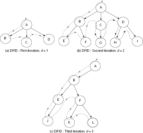
Fig. 11.20. (a)–(c) Depth-first iterative deepening (DFID) search steps.
The depth-first iterative deepening algorithm expands all nodes at a given depth before it goes for expanding nodes at some deeper level. Hence, DFID search is admissible, i.e., it guarantees to find a shortest solution path to the goal. However, it does perform some wasted computations before reaching the depth where a goal exists. It has been shown that both DFS and BFS require at least as much time and space as DFID, especially for increasingly large searches. The time and space complexities of depth-first iterative deepening search are O(bd) and O(b), respectively.
11.3.5 Bidirectional Search
The search techniques discussed so far proceed from the start state to the goal state and never in the reverse direction. It is also possible to perform the search in the reverse direction, i.e., from the goal state towards the start state provided that the state space satisfies the following conditions:
- There is a single goal state and that is provided in explicit terms so that we know at the very outset exactly what the goal state is.
- The links between the states of the search space are bidirectional. This means that the operators, or rules, provided for generation of the nodes have inverses.
A search procedure which proceeds in two opposite directions, viz., one from the start state towards the goal state (forward direction) and the other from the goal state towards the start state (backward direction), simultaneously, is called a bidirectional search. The search ends successfully when a common node is generated by both. The path from the start state to the goal state is obtained by combining the forward path from the start state to the common node α and that from the goal node to node α. The basic idea of a bidirectional search is shown in Fig. 11.21.
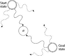
Fig. 11.21. Bidirectional search.
Example 11.3 (Bidirectional search for block manipulation problem)
Let us consider Fig. 11.5 depicting the state space of a block manipulation problem with three blocks. Assuming that node A is start state and node L the goal, we want to find a path from A to L using the bidirectional search strategy.
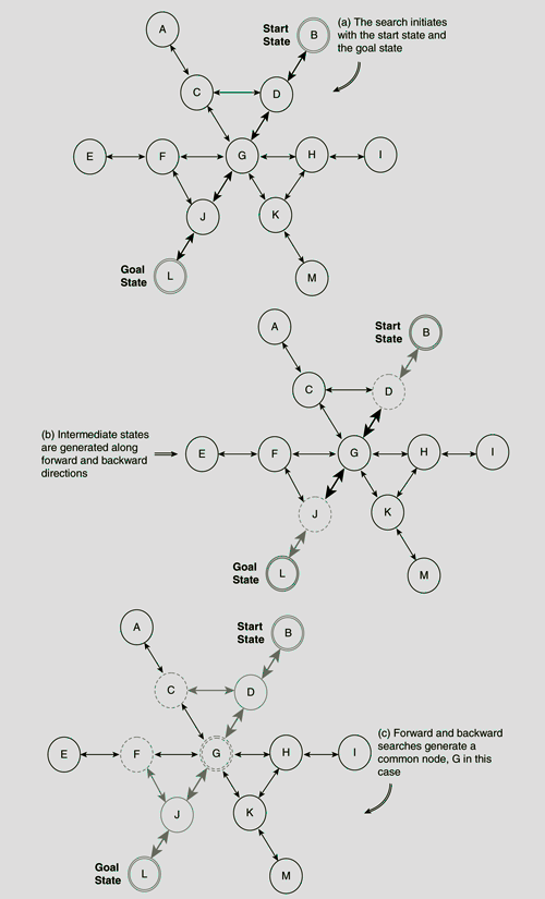
Fig. 11.22. (a)–(c) Bidirectional search for block manipulation problem.
The consecutive steps are shown in Fig. 11.22(a)–(c). The portion of the search space which remains unexplored at any instant appears in a lighter tone. Nodes that have been generated but not yet explored are depicted in dashed lines. The common node G generated by both the forward and the backward search process is drawn with double dashed lines. The path from the start node B to the goal node L consists of the sequence of nodes B-D-G-J-L which is constructed by combining the path B-D-G and L-J-G returned by the forward and backward searches, respectively.
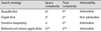
11.3.6 Comparison of Basic Uninformed Search Strategies
All the three exhaustive searches, viz., breadth-first, depth-first and depth-first iterative deepening, may be used to perform bidirectional searches with suitable modifications. The advantage of bidirectional search is that it reduces the time complexity from O(bd) to O(bd/2). This is because both the forward and the backward searches are expected to meet midway between the start state and the goal. Table 11.4 presents a comparative picture of the approximate complexities and admissibility of the basic uninformed search strategies. Here b is the branching factor, i.e., the number of children a node may have, d is the length of the shortest solution path, and D is the depth limit of the depth-first search.
Table 11.4. Comparison of basic uninformed search strategies
11.4 HEURISTIC SEARCH
Breadth-first, depth-first and iterative deepening depth-first searches discussed so far belong to the category of uninformed, or blind, searches. They try to explore the entire search space in a systematic, exhaustive manner, without employing any knowledge about the problem that may render the search process more efficient. They are blind in the sense that they do not try to distinguish good nodes from bad nodes among those still open for exploration. However, in many practical situations exhaustive searches are simply not affordable due to their excessive computational overhead. It may be recalled that they all have exponential time complexity. Heuristic search employs some heuristic knowledge to focus on a prospective subspace of the state space to make the search more efficient. In this section, the elementary heuristic searches are presented.
11.4.1 Best-first Search
Algorithm Basic-State-Space-Search (Fig. 11.14) uses the list OPEN to store nodes that have been generated, but neither been explored nor expanded. At any iteration, the first node stored in OPEN is selected for exploration and subsequent expansion. As OPEN is expected to contain several nodes at a time, a strategy must be devised to determine which among the open nodes should emerge as the first. In case of BFS, OPEN is implemented as a queue so that the most recently generated nodes are placed at the rear of OPEN, and the states of the search space are processed in first-in first-out basis. In DFS and DFID, OPEN acts as a stack so that the states are processed in last-in first-out manner. None of these strategies make any judgment regarding the relative merits of the nodes in OPEN.
Best-first search is a kind of informed search that tries, at the beginning of each iteration, to estimate the prospect of an open node with respect to reaching the goal through it. It makes use of an evaluation function that embodies some domain-specific information to achieve this. Such information is sometimes referred to as heuristic knowledge and a search procedure that is guided by some heuristic is termed as a heuristic search. The nature and significance of heuristic knowledge will be discussed in greater details in the later parts of this section. The heuristic knowledge enables us to assign a number to each node in OPEN to indicate the cost of a path to the goal through the node. In best-first search, this cost is estimated for each member of OPEN and the members are reshuffled in ascending order of this value so that the node with the lowest estimated cost is placed at the front of the queue. Therefore, Step 7 of Algorithm Basic-State-Space-Search can be written for best-first search as follows (Fig. 11.23):
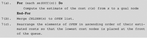
Fig. 11.23.
The behaviour of a best-first search algorithm is illustrated in Fig. 11.24(a)–(e) with the state space of Fig. 11.15 assuming node M as the only goal node. The process initiates with the start node A with an estimated cost of, say, 10. Since this is the only node available at this moment we have no option other than expanding this node. On expanding node A, the successors B, C and D are obtained with estimated costs 6, 10 and 7, respectively. Since node B has the lowest estimated cost 6, it is selected for expansion (Fig. 11.24(b)). The candidature of B for processing in the next step is indicated by the small arrow coming out of it. This convention is followed in the rest of these diagrams. Nodes E and F are generated as children of B. As shown in Fig. 11.24(c) E and F have estimated costs 8 and 9, and consequently, node D with cost 7 becomes the lowest-cost unexplored node in OPEN. Node D generates the successors H (estimated cost 3) and I (estimated cost 5). There are now five nodes, viz., H, I, E, F, and C with costs 3, 5, 8, 9 and 10, respectively of which is H is the candidate for further expansion at this moment. On expansion, node H generates M which is a goal. In this example, for the sake of simplicity, the costs are assumed. In practice, these are to be evaluated with the help of a function embodying the heuristic knowledge.
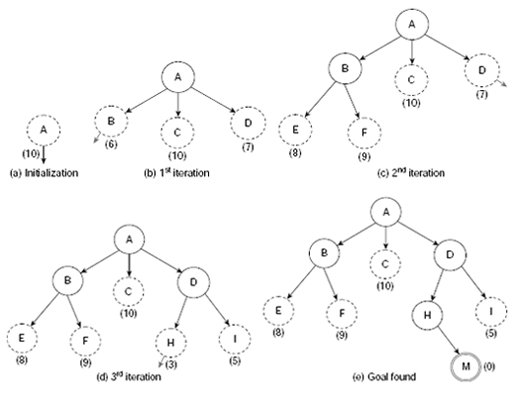
Fig. 11.24. (a)-(e) The best-first search (BFS) process.
11.4.2 Generalized State Space Search
Algorithm Basic-State-Space-Search (Fig. 11.14) hides some finer aspects of state space search for the sake of simplicity. Algorithm Generalized-State-Space-Search (Fig. 11.25) takes some of these aspects into consideration and presents a more complete picture of state space search. For example, quite often attaining a goal state alone is not sufficient. The process is to return the path from the start state to the goal state as well. In order to achieve this, we should keep track of the chain of ancestors of a node way up to the root. In Step 5 of Algorithm Generalized-State-Space-Search we first test the current node to determine if it is a goal and then, in case it is, we retrieve the path from the root to this goal by tracing the pointers from the goal to the root through the intermediate ancestors. Establishment of these pointers is done in Step 10 of the algorithm. Again, Algorithm Basic-State-Space-Search tacitly assumes the state space to be a tree rather than a graph so that the possibility of generating a node which is already present in the OPEN queue has been overlooked. As a result all nodes generated from node n, CHLDRN (n), are summarily put into OPEN. However, consider the case depicted in Fig. 11.26, where node C is a successor of node A as well as B. Let us assume that node A has been explored earlier and B later. When node B is expanded, it will produce a number of successors of which C is one. Since C is a child of A and A has been expanded earlier, C is already in OPEN. Therefore, there is no need to include C into the search tree. Moreover, while merging the children of B with the existing nodes of OPEN node, C should be left out to avoid repetitions. This is achieved in Step 8, which ensures that installation of a node and establishment of a pointer to its parent is done only if the node is not already in G. There is another possible adjustment to be incorporated. The existing pointer from C to A might be required to be redirected to B, if necessary. This depends on which among the path through A or B seems to be more promising (Step 14 of Algorithm Generalized-State-Space-Search).
11.4.3 Hill Climbing
Hill climbing is a heuristic search technique that makes use of local knowledge in its attempt to achieve global solution of a given problem. Imagine you are trying to reach the top of a hill in foggy weather. You are too small to see the peak while you are crawling on the surface of the hill and there is no clue regarding any path towards the peak. How should you proceed? One possible way would be to look around your current position and take that step which elevates you to a higher level. You continue in this way until a point is arrived from where all steps result in positions at lower heights. This point is considered to be the maximal point and corresponds to the solution to be returned. The hill climbing strategy is also applied to problems where the purpose is to reach the lowest point, and not the highest point. In such cases, steps which take us to lower heights are followed. This is sometimes referred to as valley descending. In this text we shall use the term hill climbing to mean both hill climbing and valley descending and interpret it in the context of the nature of the problem.
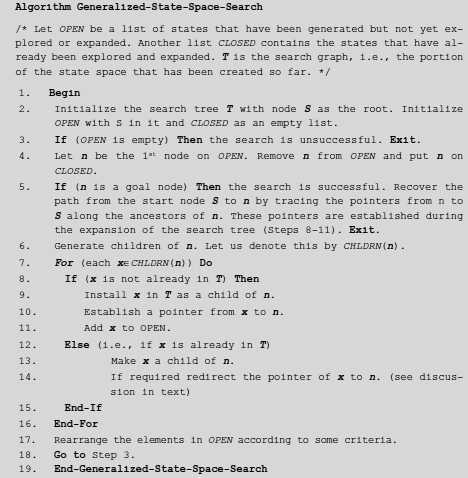
Fig. 11.25. Algorithm generalized-state-space-search.
The hill climbing strategy is widely employed to solve complex optimization problems. A hill climbing search must have the following elements.
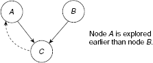
Fig. 11.26. Two nodes having a common successor.
- An objective function whose value is to be optimized. The objective function should somehow reflect the quality of a solution to the given problem so that the optimized solution corresponds to the optimal value of the objective function.
- A procedure to map a solution (perhaps sub-optimal) of the given problem to the corresponding value of the objective function.
- A procedure to generate a new solution from a given solution of the problem.
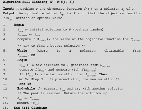
Fig. 11.27. Hill-climbing (P, f(Sp), Sp)
The hill climbing strategy is presented as Algorithm Hill-Climbing (P, f(Sp), Sp) (Fig. 11.27). It starts with a solution, perhaps randomly generated. At each intermediate step during the search process, a new solution Snew is obtained from the current one Scurrent (if possible). The quality of the new solution Snew, in terms of the evaluation function, is compared to that of the current solution. If the new solution is better than the current then the current solution is updated to the new solution (Steps 9 and 10) and the search continues along this new current solution. Otherwise, i.e., if the new solution is not better than the current solution, then it is discarded and we generate yet another new solution (if possible) and repeat the steps stated above. The process stops when none of the new solutions obtained from the current one is better than the current solution. This implies that the search process has arrived at an optimal solution. This is the output of the hill climbing process.
It may be noted that the hill climbing method does not create a solution tree. The only things it maintains are the current and the newly generated solutions. If the new solution is better than the current then it discards the current solution and update it with the new solution. In other words, hill climbing grabs a good neighbour without bothering the aftereffects. For this reason hill climbing is also referred to as greedy local search.
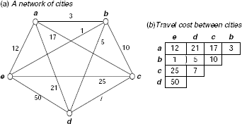
Fig. 11.28. A tiny traveling salesperson problem (TSP) with five cities.
Example 11.4 (A hill climbing technique to solve the TSP)
As an example, let us consider the traveling salesperson problem (TSP), which involves a network of cities connected to each other through paths with costs attached to them. A tour is defined as a path that starts from a given city, travels through the paths to visit every other city exactly once, and returns to the starting city. We are required to find a minimal cost tour.
Fig. 11.28 (a) shows a tiny TSP with five cities a, b, c, d, and e. For the sake of simplicity the cities are taken to be fully connected, i.e., an edge exists between any pair of cities. If we start at the city a then a tour may be represented with a permutation of the letters a, b, c, d, and e that starts and ends with the letter a.
The TSP is a minimization problem. Its objective function is the sum of the costs of the links in the tour. For example, if the tour is τ = abcdea then its cost cost(τ) = cost(ab) + cost(bc) + cost(cd) + cost(de) + cost(ea) = 3 + 10 + 7 + 50 + 12 = 82. Mapping a solution to evaluate the objective function is also straightforward in this case. How to generate a new solution of the TSP from a given one?
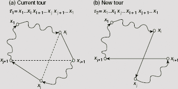
Fig. 11.29. Generation of a new tour from a given tour.
Let τ1 = x1… xi xi+1… xj xj+1… x1 be an existing tour. A new tour τ2 from τ1 could be generated in the following manner.
- Let xi xi+1 and xj xj+1 be two disjoint edges in τ1 such that the cities xi, xi+1, xj and xj+1 are all distinct.
- Remove the edges xi xi+1 and xj xj+1 from the tour τ1.
- Join the edges xixj and xi+1xj+1 such that a new tour τ2 = x1…xixj…xi+1xj+1…x1 is obtained.
Fig. 11.29 shows the procedure graphically. Now, to illustrate the hill climbing procedure we may consider the of TSP presented in Fig. 11.28. The successive steps are shown in Fig. 11.30 (a)–(e). A random solution adecba denoting the tour a → d → e → c → b → a is considered as the initial solution (Fig. 11.30(a)). The cost of the tour is 109. To obtain a new tour the links ad and ec are are removed from the tour and are substituted by ae and cd. So we obtain the tour abcdea with cost 82 (Fig. 11.30(b)). Since this cost is lower (and hence, better, since we are addressing a minimization problem) we accept this solution and proceed.
In this way, we proceed to acdbea (Fig. 11.30(d)) having a tour cost of 42. Only three tours, viz., acebda, abedca, and acbdea shown in Fig. 11.30 (e1), Fig. 11.30(e2), and Fig. 11.30(e3) can be generated from this tour. These three tours have costs 69, 78 and 94, respectively. Since all of these are higher than 42, the hill climbing procedure assumes to have reached a minimal value and the procedure stops here. It is easy to verify that the other possible tours have costs greater than 42. The solution returned by the hill climbing process is thus acdbea and the cost of the solution is 42. The successive steps shown in Fig. 11.30(a)–(e) are given here for the sake of understanding the process but these are not memorized by the actual hill climbing procedure.
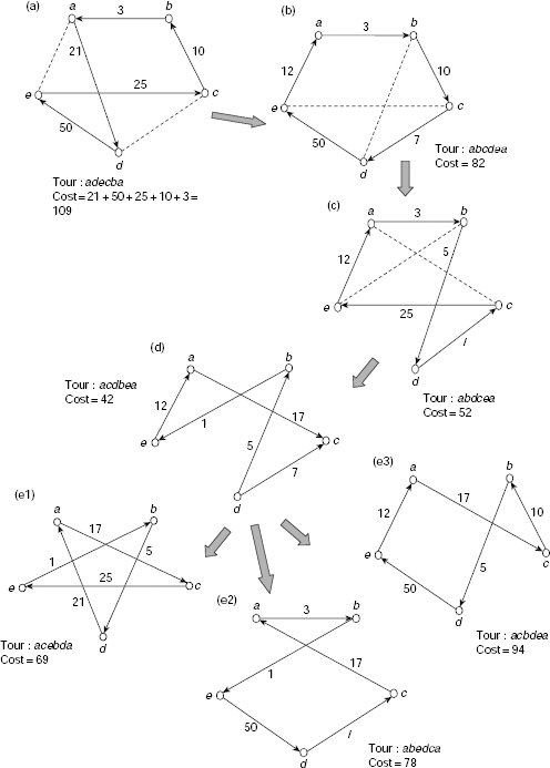
Fig. 11.30. Solving TSP through hill climbing.
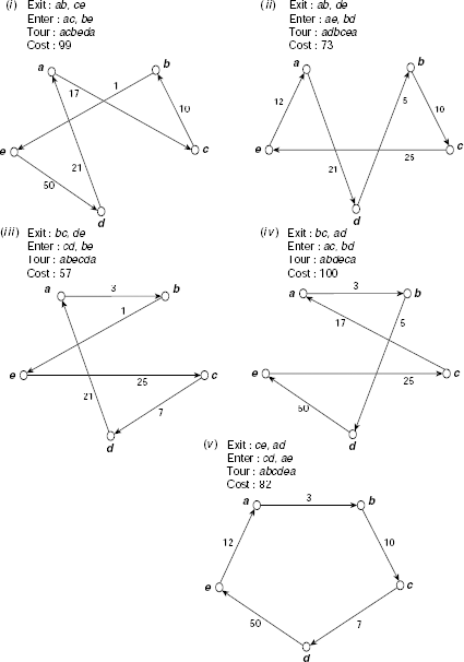
Fig. 11.31. Various solutions obtained from the tour adecba
Steepest ascent hill climbing In Algorithm Hill-Climbing a new solution is generated from the current solution and if it is found to be a better solution then the search proceeds along this new solution without any consideration of any other possible solution obtainable from the current one. Steepest ascent hill climbing is a variation of hill climbing, where instead of one all possible solutions from the current solution are generated and the best among these is chosen for further progress.
For example, if we follow the steepest ascent hill climbing strategy on the initial tour adecba shown in Fig 11.30(a), then the entire set of tours that can be obtained from adecba should be generated and their costs be evaluated. Five different tours, acbeda, adbcea, abecda, abdeca, and abcdea, can be generated by transforming adecba. These tours have costs 99, 73, 57, 100 and 82, respectively (see Fig. 11.31(i)–(v)). Obviously, tour abecda of cost 57 would be selected for further exploration.
Local optima / plateaux / ridges Hill climbing is usually quite efficient in the search for an optimal solution of a complex optimization problem. However, it may run into trouble under certain conditions, e.g., existence of local optima, plateaux, or ridges within the state space.
Local optima. Often the state space of a maximization problem has a peak that is higher than each of its neighbouring states but lower than the global maximum. Such a point is called a local maximum. Similarly a minimization problem may have local minima. Fig. 11.32 shows a one-dimensional objective function containing local optima and plateaux. Since the hill climbing procedure examines only the solutions in the immediate neighborhood of the current solution it will find no better solution once it reaches a locally optimal state. As a result, there is a chance that the local optima, and not the global optima, is erroneously identified as the solution of the problem.
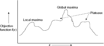
Fig. 11.32. Problem of local optima and plateaux.
Plateaux. A plateau is a flat region in the state space (Fig. 11.32) where the neighbouring states have the same value of the objective function as that of the current state. A plateau may exit at the peak, or as a shoulder, as shown in Fig. 11.32. In case it is a peak, we have reached a local maximum and there is no chance of finding a better state. However, if it is a shoulder, it is possible to survive the plateau and continue the journey along the rising side of the plateau.
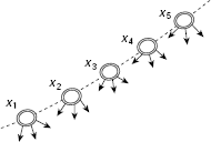
Fig. 11.33. A ridge.
Ridges A ridge is a series of local optima on a slope. Consider a situation depicted in Fig. 11.33. Each of the states x1, x2, x3, x4, and x5 is a local maximum and they are arranged in the state space from left to right in ascending order. We would like to ascend along the path x1 → x2 → x3 → x4 → x5 etc., but all the states leading from each of these states, indicated by the arrows, are at lower levels in comparison with these states. This makes it hard for the search procedure to ascend.
The problems arising out of local optima, plateaux, or ridges may be addressed by augmenting the basic hill climbing method with certain tactics. However, though these tactics help a lot, they do not guarantee to solve the problems altogether. Here is a brief description of the way outs.
- The problem of getting stuck at local optima may be tackled through backtracking to some previous state and then take a journey along a different direction but as promising, or almost as promising, as that chosen earlier.
- To escape a plateau, one may make a big jump in some direction and land on a new region of the search space. If there is no provision of making a big jump, we may repeatedly take the allowable smaller steps in the same direction until we come outside the plateau.
- A good strategy to deal with ridges is to apply several rules before doing a test so that one can move in different directions simultaneously.
11.4.4 The A/A* Algorithms
While discussing best-first search, we have seen how an evaluation function can guide the search process along a more fruitful path than exploring the entire search space blindly. However, we did not mention the form of the evaluation function. Let us define the evaluation function f(n) for a given node n as
where g(n) is the cost of a minimal-cost path from the start node to node n and h(n) is the cost of a minimal-cost path from node n to a goal node.
Therefore, f(n) is the cost of a minimal-cost path from the start node to a goal node constrained to pass through node n (Fig. 11.34).
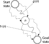
Fig. 11.34. A minimal-cost path from start to goal passing through node n.
However, sometimes it is difficult if not impossible to evaluate g(n) and h(n) accurately. Therefore some estimated values of g(n) and h(n) are used to guide the search process. Let g1(n) and h1(n) be the estimated values of g(n) and h(n). Then the estimated value of f(n), written as f1(n), is defined as
A search algorithm that uses f1(n) to order the nodes of OPEN queue and chooses the node with best value of f1(n) for further exploration is called an A algorithm. Moreover, if the heuristic estimation h1(n) happens to be a lower bound of h(n) so that h1(n) ≤ h(n) for all n, then it is termed as A* (pronounced as a-star) algorithm. An obvious example of A* algorithm is BFS. Here g1(n) is the depth of node n from the root node and h1(n) = 0 for all n. Since h1(n) ≤ h(n) for all n, BFS satisfies the basic criterion of A* algorithm. It has been proved that an A algorithm satisfying the relation h1(n) ≤ h(n) for all n, is guaranteed to find an minimal-cost path from the root to a goal. Such a search algorithm is said to be admissible and hence A* algorithm is admissible.
Example 11.5 (An A-algorithm to solve 8-puzzle)
Let us consider the 8-puzzle posed in Fig 11.11. We would like to solve it through an A algorithm. The first component of the evaluation function f(n) = g(n) + h(n) is g(n), is defined as
Regarding the second component, h(n), we must employ some heuristic knowledge that somehow gives an idea of how far the goal node is from the given node. Presently, we take the number of tiles that are not in positions described in the goal state as the distance from the goal node. Therefore, the function h(n) is defined as
Now, consider the initial state of the given instance of 8-puzzle and compare it with the goal state (Fig. 11.35).
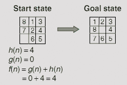
Fig. 11.35. Evaluating the heuristic function h(n).
Since the start state is to the root of the search tree g(n) = 0 for this node. To evaluate h(n) we count the number of misplaced tiles. A comparison with the goal state reveals that tile no. 1, 2, 7, and 8 are not in their positions. Therefore, h(n) = 4, so that f(n) = 0 + 4 = 4. Expanding the start state we get two new states with h(n) values 3 and 5, respectively. Since both of these nodes are at level 1 of the search tree, g(n) = 1 for both of them. Hence these two nodes f(n) = g(n) + h(n) = 1 + 3 = 4, and 1 + 5 = 6, respectively. The node with the lesser f(n) value 4, is chosen by the algorithm for exploration. The successive steps while constructing the search tree are shown in Fig. 11.36 (a)-(e).
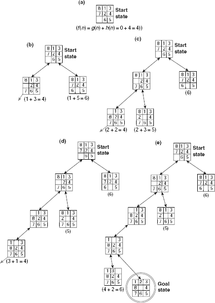
Fig. 11.36. (a)-(e) Steps of A-algorithm to solve the 8-puzzle.
Example 11.6 (An A* Algorithm to solve a maze problem)
Fig. 11.37 shows a 5 × 5 maze with a barrier drawn with heavy lines. We have to find a path from cell (4, 2)to cell (2, 3) avoiding the barrier. At each step of the journey we are allowed to move one cell at a time left, right, up, or down, but not along any diagonal. One or more of these movements may be blocked by the barrier. Fig. 11.38(a) and Fig. 11.38(b) explains the rules of movement. The target is to find a minimal length path from the source to the destination under the restriction imposed by the barrier. An A* algorithm is to be found to do the job.
The length of a path from a cell (i, j) to a cell (k, l) is the number of cells traversed along the path. For example, the path shown by the dotted line of Fig. 11.39 between the cells (2, 1) and (4, 5) has a length of 10. Let us take the estimated value of g(n)
where n0 and n are the initial and the current cell positions, respectively.
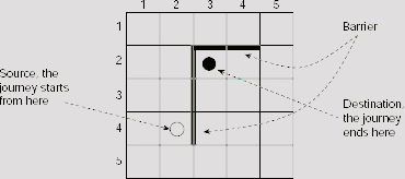
Fig. 11.37. A maze problem to find the shortest path from the source to destination avoiding the barrier.
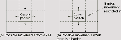
Fig. 11.38. Possible movements from a cell.
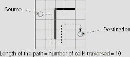
Fig. 11.39. Length of a path.
The heuristic estimation function h1(n) is defined as
Hence, if D(i), D(j) and n(i), n(j) are the row numbers and column numbers of the cells D and n, respectively, then h1(n) is calculated as
It is easy to see that h1(n) is the minimum number of cells we must traverse to reach D from n in absence of any barrier. Therefore, h1(n) ≤ h(n) for every n. This implies that the evaluation function
satisfies the criteria for A* algorithm. In the present instance of the problem, the source n0 is the cell (4, 2) and the destination D is the cell (2, 3). At the source, g1(n0) = 0, and h1(n) = | 2 − 4 | + | 3 − 2 | = 3, so that f1(n) = 0 + 3 = 3. From this initial position, we may try to move to cell (5, 2), (4, 1), or (3, 2). Moving to cell (4, 3) is prohibited by the barrier between cells (4, 2) and (4, 3). Now, as indicated in Fig. 11.40(b), the value of f1(n) for these cells are 4, 5, and 3, respectively. As 3 is the lowest among these, the corresponding cell (3, 2) is selected for further exploration.
As far as the shortest route to the destination is concerned, this is not the right choice because the intervening barrier will not allow us to take to take the shortest route. The right choice would be to proceed along the cell (5, 2). However, the merit of (5, 2) over other choices is not apparent till the step shown in Fig. 11.40(i), where all OPEN nodes except (5, 2) have cost 7 and (5, 2) have a cost of only 5. Superiority of the path along (5, 2) is maintained for the rest of the search, until we eventually reach the goal (Fig. 11.41).
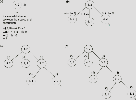
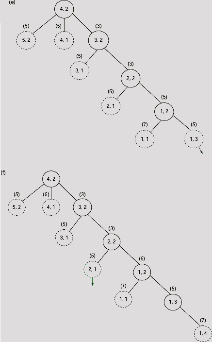
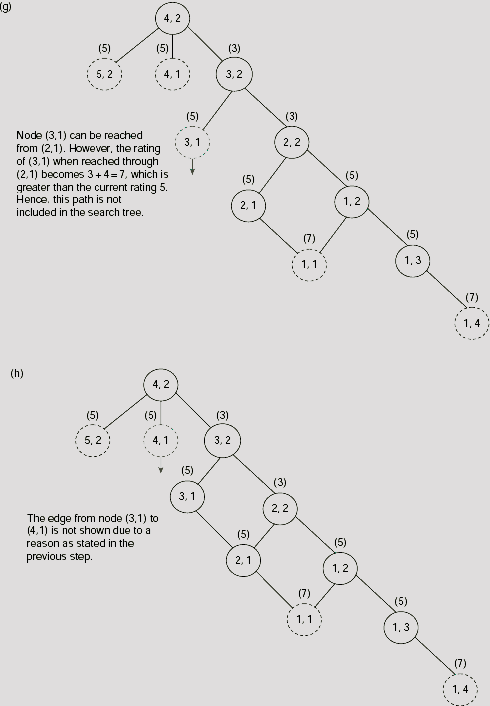
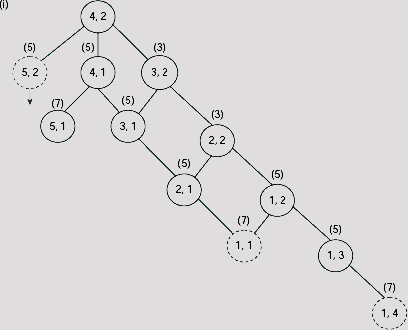
Fig. 11.40. (a)-(i) Trace of the first nine steps of A* search for the maze problem.
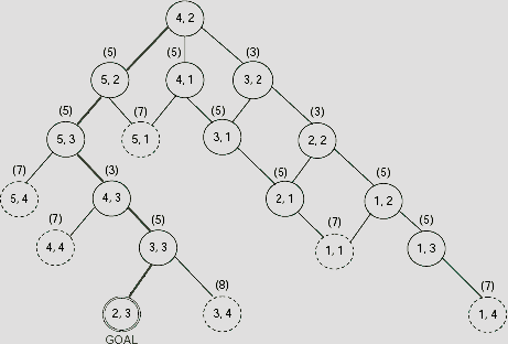
Fig. 11.41. Search tree for the maze problem.
The path from the root to the goal is shown with thick lines in Fig. 11.41. The corresponding minimum length path in the maze is shown with dotted lines of Fig. 11.42.
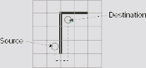
Fig. 11.42. The minimum length path found through the A* algorithm
Example 11.7 (Branch-and-bound algorithm for traveling salesperson problem)
Let us consider the TSP once more. We want to design an A* algorithm to solve the TSP and apply it on the network shown in Fig. 11.43. Let C1, C2, …, Ck be k cities and ci,,j denotes the cost of the link between Ci and Cj. Without loss of generality, let us suppose that the tour starts at C1 and let τ = C1 → C2 → … → Ci be a partial path generated the search process. Then the cost of the path τ = C1 → C2 → … → Ci is given by
In branch-and-bound technique, a list of possible paths from the starting city is maintained during the search process. Cost of each partial path is found and the so far minimum cost path is chosen for further expansion. While we expand a certain path, we temporarily abandon the path as soon as it is found to exceed the cost of some other partial path. The algorithm proceeds in this way until the minimum-cost tour is obtained. It should be noted that the decision to select a partial path τ = C1 → C2 → … → Ci is made solely on the basis of its cost g(τ) and no estimation of the cost for the remaining portion of the tour is done. Therefore h1(τ) = 0 for every partial path. Since h1(τ) = 0 ≤ h(τ), this is an A* algorithm, and it guarantees to find the minimal cost tour for a given TSP.
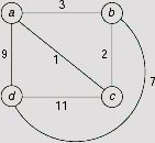
Fig. 11.43. A network of four cities.
For this example, the algorithm starts with the starting city a, and since no path is yet traversed the cost attached to this node is 0 (Fig. 11.44 (i)). From city a we can either go to city b, or c, d. The cost of the paths a → b, a → c, and a → d are 3, 1, and 9, respectively. Since the path a → c has the lowest cost of 1 so far, this path is chosen at this point for further extension. This is indicated by a small arrow attached to the node c in Fig. 11.44(ii), which shows the initial two steps of the algorithm.
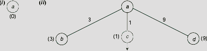
Fig. 11.44. First two steps of branch-and-bound
Fig. 11.45(i) shows the situation when we proceed one step further along the partial path a → c. The two extended paths a → c → b and a → c → d have total estimated costs 1 + 2 = 3 and 1 + 11 = 12, respectively. As the cost of the partial path a → c → b does not exceed that of the remaining paths (3 for a → b, 12 for a → c → d, and 9 for a → d) it is selected for further expansion at this point and the result of this expansion is shown in Fig. 11.45(ii). Fig. 11.45(iii) and 11.45(iv) shows two more consecutive steps.
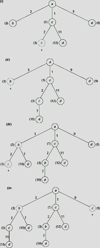
Fig. 11.45. Further steps TSP through branch-and-bound.
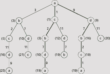
Fig. 11.46. Final branch-and-bound search tree.
The final branch-and-bound search tree is depicted in Fig. 11.46. The tours generated are a → c → b → d → a and a → d → b→ c → a with the cost 19. It should be noted that these two tours are the same tour, only traversed in reverse directions. The lowest-cost tour obtained thus is shown in Fig. 11.47.
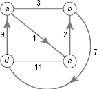
Fig. 11.47. The lowest-cost tour.
The efficiency of a heuristic search heavily depends upon the choice of the heuristic estimation function h1. The function h1 embodies some heuristic knowledge about the problem. Its objective is to guide the search for goal in the right direction. It is expected that a better heuristic will result in less amount of wasted effort in terms of the exploration of nodes that do not belong to the optimal path from the start state to a goal state. Let us consider two A* algorithms A1 and A2 using the heuristic functions h1 and h2, respectively. We say that algorithm A1 is more informed than A2 if for all nodes n except the goal node h1(n) > h2(n). Please note that for any A* algorithm the estimate h1(n) of h(n) must be a lower bound of h(n), the actual cost of a minimal cost path from node n to a goal node. Combining this with the above inequality we get 0 ≤ h2(n) < h1(n) ≤ h(n). In other words, better heuristics are closer to h(n) than a worse one.
11.4.5 Problem Reduction
A problem is said to be decomposable if it can be partitioned into a number of mutually independent sub-problems each of which can be solved separately. Decomposing a problem into sub-problems is advantageous because it is generally easier to solve smaller problems than larger ones. The problem reduction strategy is based on this characteristic. It employs a special kind of graph called AND-OR graph. The search through an AND-OR graph is known as AO* search.
AND-OR Graphs. There are two kinds of relation between the decomposed sub-problems and the problem itself. Firstly, the solution of any of the sub-problems may provide the solution of the original problem. This is an OR relationship. On the other hand, it might be necessary to solve all the sub-problems to obtain the final solution. This is called the AND relationship.
Each node of an AND-OR graph represents a problem. The root node represents the given problem while all other nodes represent sub-problems. Given a node and its children, if there is an OR relationship among them then the related arcs are called OR-links. In case of AND relationship these are called AND-links. The standard representations for these two types of links are shown in Fig. 11.48(a) and Fig. 11.48(b). It is possible that a node issues OR-links as well as AND-links simultaneously. Fig. 11.48(c) shows such a situation.
To illustrate the AND-OR graphs let us consider a network of four cities a, b, c and d and their interconnection cost as shown in Fig. 11.49. How to find a lowest-cost route from city a to city d?
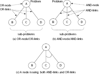
Fig. 11.48. Representation of AND/OR nodes/links in AND-OR graphs.
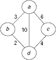
Fig. 11.49. A network of four cities.
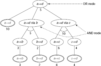
Fig. 11.50. AND-OR tree for reaching city d from city a.
Fig. 11.50 shows the AND-OR graph for the given problem. City d can be reached in three different ways, viz., along the direct path from a to d, or, from a to d via b, or, from a to d via c. So the given problem a → d is now decomposed into three disjoint sub-problems, ‘a → d’, ‘a → d via b’, and ‘a → d via c’. In Fig. 11.50 this is shown as the three children of the root node. Since the given problem can be solved through any of these three sub-problems, we have an instance of an OR node. Moreover, as there is a direct path from a to d with cost 10, a solution to the problem is readily available. This is indicated by the highlighted ovals.
Let us now focus on the sub-problem ‘a → d via b’. In order to reach d via b, we have to reach b from a, and then from b to d. This is indicated by the two children of the node for ‘a → d via b’. The fact that both of the sub-problems a → b and b → d have to be solved to obtain a solution of ‘a → d via b’ implies that this is an AND node. Each of the two children leads to a leaf node as shown in the figure. The weights attached to an AND node is the sum of the weights of its constituent children. On the contrary, the weight attached to an OR node is the best among its children. In the present context we are looking for the minimum-cost path from a to d, and therefore, the cost 5 (among 10, 5, and 10) is attached to the root node. The entire AND-OR tree is depicted in Fig. 11.50. In the present example, the cost is attached to the nodes. However, depending on the nature of the problem addressed, one may attach such weights to the arcs also.
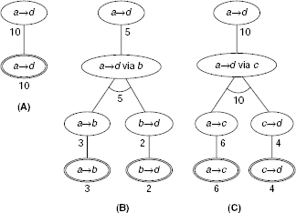
Fig. 11.51. Solution trees for reaching city d from a.
How to obtain the solution to a problem represented by an AND-OR graph ? Since a solution must include all the sub-problems of an AND node, it has to be a subgraph, and not simply a path from the root to a leaf. The three different solutions for the present problem are shown as the solution trees A, B and C in Fig. 11.51. As we are addressing the problem of finding the minimum-cost path, Solution (B) will be preferred. We can formally define such solution graphs in the following way:
Let G be a solution graph within a given AND-OR graph. Then,
- The original problem, P, is the root node of G.
- If P is an OR node then any one of its children with its own solution graph, is in G.
- If P is an AND node then all of its children with their own solution graphs, are in G.
In this example, we have considered an AND-OR tree rather than a graph. However, AND-OR graph is the more generalized representation of a decomposable problem.
The AO* Algorithm. Typically, state space search is a search through an OR graph. The term OR graph is used to indicate the fact that if there is a node n with k number of edges e1, …, ek incident on it, then n can be reached either along the edge e1, or along e2, or … or along ek (Fig. 11.52(a)), i.e., along any of the edges e1, …, ek. In contrast, if there is an AND node n within an AND-OR graph with k number of edges e1, …, ek incident on it, then in order to attain n one has to reach it along the edge e1, and along e2, and … and along ek (Fig. 11.52(b)), i.e., along all of the edges e1, …, ek.
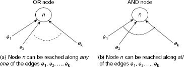
Fig. 11.52. Difference between OR-node and AND-node.
Depth-first search, breadth-first search, best-first search, A* algorithm etc. are the well-known search strategies suitable for OR graphs. These can be generalized to search AND-OR graphs also. However, there are certain aspects which distinguish an AND-OR search from an OR graph search process. These are:
- An AND-OR graph represents a case of problem reduction through decomposition. Hence each node of such a graph represents a problem to be solved (or already solved). On the other hand a node of an OR graph represents the state of a problem within the corresponding state space.
- The goal of searching an OR graph is to find a path from the start node to a goal node where such a path is required, or simply to reach a goal node. On the contrary, the outcome of an AND-OR graph search is a solution tree rather than a path, or goal. The leaves of such trees represent the trivially solvable problems which can be combined to solve a higher-level problem and so on until we come to the root node which represents the given problem.
Before we present the algorithms for AND-OR graph search in a formal way, let us try to grasp the main idea with the help of an example.
Example 11.8 (Searching through AND-OR graph)
Fig. 11.53 shows a network of six cities a, b, c, d, e, and f. The weight associated with each edge denotes the cost of the link between the corresponding cities. We are to find a minimum-cost path from a to f.
The AND-OR graph representation of this problem is shown in Fig. 11.54. Here we have tried to find a path from a to f without considering the issue of finding minimum cost path. There must be systematic procedure to construct an AND-OR graph and moreover, once we arrive at a solution to the given problem in course of this construction process there is no need to construct the rest of the search tree. In other words, we don’t have to construct the entire AND-OR graph in practice.
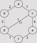
Fig. 11.53. Interconnection of cities and related costs.
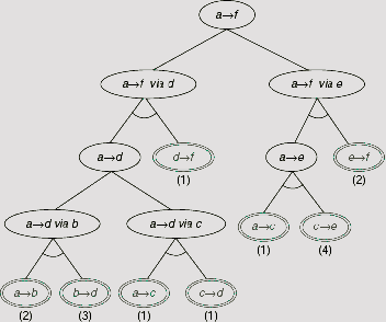
Fig. 11.54. AND-OR graph for the problem.
The step-by-step construction of the AND-OR graph as well as arrival at the solution of the given problem is illustrated in Fig. 11.55(a)–(f). The search for a minimum cost path from a to f starts with the root of the AND-OR graph. We employ a heuristic function h1 associated with each node of the graph. For a node n, h1(n) estimates the cost of the path from node n to node f. Given a node n, h1(n) is estimated as
where w is the average cost of a link between two cities, and d = the estimated number of edges between node n and the goal node. The average edge-weight is calculated as
Moreover, we assume a uniform cost of 1 for each link of the AND-OR graph. While estimating the cost of an internal node, those of its descendant along with the costs of the links are taken into consideration.
As there are six cities, at most five edges may exist in a path between node a, and node f. Hence the estimated cost h1(n) = d × w = 5 × 2 = 10 is attached to the root node (see Fig. 11.51(55)(a)). In the next step the initial task a → f is split into two sub-tasks (a → f via d) and (a → f via e) because f can be reached either through d or through e. This is represented in Fig. 11.51(55)(b) by the successors of the root node. As f can be approached along any one of the paths through d or e, the corresponding sub-tasks are attached to their parent through OR-links. The estimated cost of the node (a → f via d) is obtained as h1(a → f via d) = h1(a → d) + (cost of edge df) = 4 × 2 + 1 = 9. Since the length of a path from a to d is 1 less than that from a to f we have taken d = 4. Similarly, the cost estimate of the node (a → f via e) is calculated as 4 × 2 + 2 =10. If we proceed along node (a → f via d) then the estimated cost at the root is (9 + 1) = 10. The cost of traversing along the sub-problem (a → f via e) is (10 + 1) =11. Since we are looking for the minimum cost path, the former is the right choice. This is indicated by the broken arrow along the link from the root node to the node (a → f via d). Moreover, the estimated minimum cost 10 is now associated with the parent of (a → f via d).
The next step is to expand the node (a → f via d). In order to arrive at f from a via node d one has to traverse a path from a to d (i.e., task a → d) and then from d to f. Therefore node (a → f via d) is split into two sub-tasks a → d and d → f, each attached to its parent with the help of an AND link. This is shown in Fig. 11.55(c). As the node d is directly connected to f the task d → f is readily solved. This is indicated by the doubly encircled node for d → f. The cost of this task is simply the cost of the edge df, 1. The estimated cost of the other child is (4 × 2) = 8.
Once we arrived at a node marked as solved we have to move upward along the tree to register the effect of this arrival at a solution on the ancestors of the solved node. The rule is, if each successor of an AND node is solved, then the parent node is also solved. And if any successor of an OR node is solved then the parent node is solved. Modification of the status of the ancestors goes on until we arrive at the root, or a node which remains unsolved even after consideration of the solved status of its children. In the present case the parent of the solved node (d → f) is the AND node (a → f via d). Since its other child still remains unsolved the unsolved status of node (a → f via d) does not change and the process stops here.
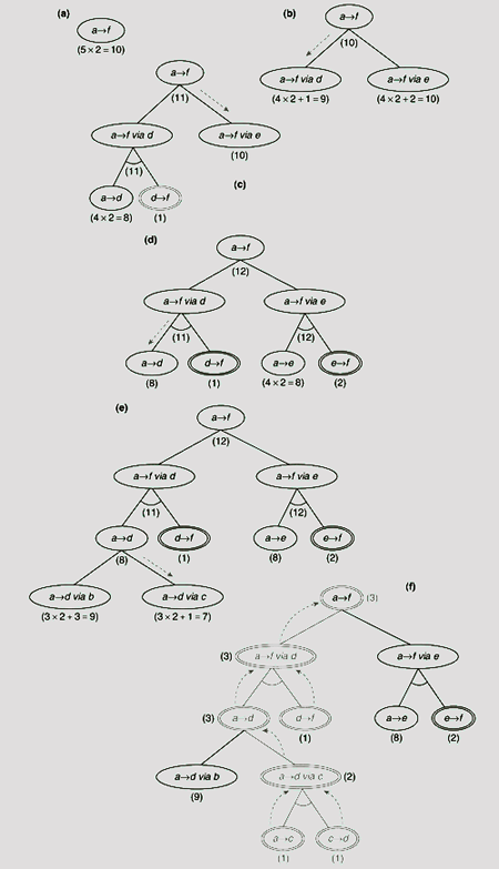
Fig. 11.55. AND-OR search for minimum-cost path between cities
The costs of the nodes are now to be revised on the basis of the estimates of the newly created nodes. The cost of (a → d) is calculated as 8 and that of (d → f) is (0 + 1) = 1. Here h1(d → f) = 0 because the sub-problem d → f is already solved. As (a → f via d) is an AND node its revised estimated cost should take into account the costs of both of its successors as well as the links. This becomes (8 + 1) + (1 + 1) = 11. When we try to propagate this value upwards, we find the cost of the root node to be (11 + 1) = 12. This is greater than the cost (10 + 1) = 11 when we approach the root along its other child (a → f via e). Thus we abandon the previous path and mark (a → f via e) as the most promising node to be expanded next (Fig. 11.55(c)). The subsequent steps are depicted in Fig. 11.55(d) to Fig. 11.55(f). Fig. 11.55 (f) conveys the outcome of the entire process. Here, when the task (a → d via c) is split into two sub-tasks a → c and c → d it is found that both of these sub-tasks are readily solved. This makes their parent AND node (a → d via c) to be marked as solved which in turn solves the parent task a → d. As we go on climbing the tree in this way the root node which represents the given problem is marked as solved – a condition which indicates the end of the search process. The outcome of the entire process, i.e., the solution tree, is highlighted in Fig. 11.55(f).
A simplified AND-OR graph search technique is described in Algorithm AO* (Fig. 11.56). It starts with the given problem as the initial node and gradually constructs the AND-OR graph by decomposing a problem into sub-problems and augmenting the partially constructed graph with the nodes corresponding to those sub-problems. At any point, nodes that are generated but not yet explored or expanded are kept in a queue called OPEN and those which have already been explored and expanded are kept in a list called CLOSED. The prospect of a node with respect to the final solution is estimated with the help of a heuristic function. Moreover, two labels, viz., SOLVED, and FUTILE are used to indicate the status of a node with respect to the solvability of the corresponding problem. A node that represents a readily solved problem need not be decomposed further and is labeled as SOLVED. On the other hand, a problem which is not solvable at all, or the solution is so costly that it is not worth trying, is labeled with FUTILE.
The operation of the algorithm can be best understood as a repetition of two consecutive phases. In the first phase the already constructed graph is expanded in a top-down approach. In the second phase, we revise the cost estimates of the relevant nodes, connect or change the connections of the nodes to their ancestors, see if some problems, or sub-problems, are readily solvable or not solvable at all and propagate the effect of these towards the root of the graph in a bottom-up fashion.
At each step we identify the most promising solution tree with the help of the cost estimates of the nodes. A yet-unexplored node of that tree is selected for further expansion. The children of this node are integrated into the existing AND-OR graph. Depending on the estimated costs of the newly introduced nodes, the cost estimates of their ancestors are recomputed. Moreover, if the current node is tagged as SOLVED, or FUTILE, then the status of its ancestors are also changed if necessary. The process stops when the initial node is labeled as SOLVED or FUTILE.
The example discussed above gives a simplified picture of AND-OR search because it works on a tree rather than a graph. Moreover, a node in an AND-OR graph may involve both AND-links and OR-links. Fig. 11.57 depicts few steps of an imaginary AND-OR graph search involving such a situation. In Fig. 11.57(a), node c is the lowest cost individual node. But selection of c compels us to select node d also because both of them forms an AND-arc together. Since the sum of the costs of these two nodes is greater than the other node b, it is selected at the moment for exploration and expansion. The situation changes after this step (Fig. 11.57(b)) and the AND-arc involving nodes c and d becomes most prospective for further processing. Since c is cheaper than d the algorithm will select c for processing.
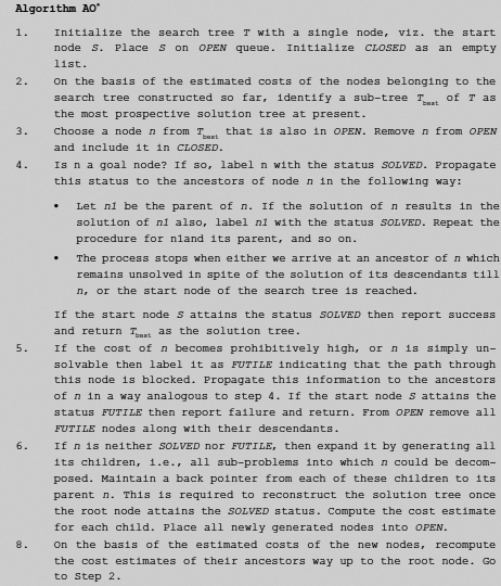
Fig. 11.56. Algorithm AO*.
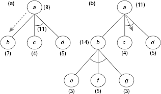
Fig. 11.57. Characteristics of AO* search
It has been found that AO* algorithm is admissible, i.e., it guarantees to find an optimal solution tree if one exists, provided h1(n) ≤ h(n) for any node n, and all costs are positive. If h(n) = 0 then AO* algorithm becomes breadth-first search. AO* is also known as the best-first search algorithm for AND-OR graphs.
11.4.6 Means-ends Analysis
Means-Ends Analysis (MEA) is a technique employed for generating plans for achieving goals. This technique was first exploited in sixties by a famous A.I system known as the General Problem Solver (GPS). The central idea underlying the MEA strategy is the concept of the difference between the start state and the goal state and in general the difference between any two states. The MEA process recursively tries to reduce the difference between two states until it reduces to zero. As a result it generates a sequence of operations or actions which transforms the start state to the goal state. The salient features of an MEA system are described below.
- It has a problem space with an initial (start) state (object) and a final (goal) state (object).
- It has the ability to compare two problem states and determine one or more ways in which these states differ from each other. Moreover, it has the capacity to identify the most important difference between two states which it tries to reduce in the next step.
- It can select an operator (action) appropriate for application on the current problem state to reduce the difference between the current state and a goal. It employs a difference-operator table, often augmented with preconditions to the operators, for this purpose. The difference-operator table specifies the operators applicable under various kinds of differences.
- There is a set of operators, sometimes referred to as rules. An operator can transform one problem state to another. Each operator (rule) has a set of pre-conditions and a set of post-conditions, or results. The pre-conditions of a rule describe the situation in which the rule can be applied. Similarly, the post-conditions describe the changes that will be incorporated into the problem state as a result of the operation applied.
The basic strategy of means-ends analysis is described in the pseudocode Algorithm Means-Ends Analysis (Scurrent, Sgoal) (Fig. 11.58) and is illustrated in Fig. 11.59.
Suppose Scurrent and Sgoal are the initial and the goal states pertaining to the given problem. A sequence of operations is to be generated that transforms Scurrent to Sgoal. The system identifies D to be the most important difference between the start state and the goal state. This situation is depicted in Fig. 11.59(a). Fig. 11.59(b) shows the situation prevailing after application of an appropriate operator OP, which is employed to reduce the gap D. Let Spre-op be the problem state that satisfies the pre-conditions for applying the operator OP and Spost-op be the problem state resultant of applying OP on Spre-op. Then the portion of D indicated by CD of Fig. 11.59(b) has been filled and the original difference D represented by the distance AB in Fig. 11.59(a) and (b) is fragmented into two gaps (may be one) D1 and D2 represented as the distances AC and DB in Fig. 11.59(b). The differences D1 and D may further be reduced by invoking MEA(Scurrent, Spre-op) and MEA(Spost-op Sgoal), respectively. It should be noted that OP will be actually included in the final plan only if both MEA(Scurrent, Spre-op) and MEA(Spost-op Sgoal) are successful and return their own sub-plans P1 and P2 so that the final plan is obtained by concatenating P1, OP, and P2.
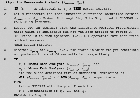
Fig. 11.58. Algorithm means-ends analysis (Scurrent, Sgoat).
The MEA process is a kind of backward chaining known as operator subgoaling that consists of selection of operators and subsequent setting up of sub-goals so that the pre-conditions of the operators are established.
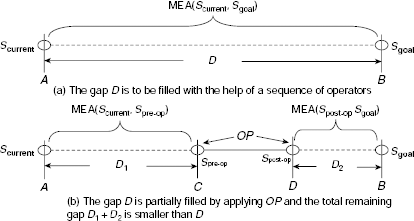
Fig. 11.59. Basic means-ends analysis strategy.
Example 11.9 (Means-Ends Analysis)
Suppose a person want to reach his friend’s house at New Delhi from his home at Kolkata. The distance between Kolkata and New Delhi is about 1500 km. Depending on the distance to be traveled and subject to availability, various kinds of conveyances are used. For example, if it is a very short distance, say, less than 1 km, one should simply walk. For a destination further than 1 km but within the locality one may use a car or a bus. Similarly, to travel larger distances a train, or an aeroplane may be used. In order to board an aeroplane we have to reach the airport. Similarly, to catch a train one has to arrive at the railway station. The airport, or the railway station, may be reached through a car, or a bus, and so on. We want to generate a plan through MEA for this problem.
Here a problem state is defined as the position, or location, of the person. For the sake of simplicity, let us consider a discrete, finite set of possible locations, say, at-home-at-K, at-the-car-at-K, at-the-car-at-ND, at-the-bus-stop-at-K, at-the-bus-stop-at-ND, at-the-station-at-K, at-the-station-at-ND, at-the-airport-at-K, at-the-airport-at-ND, at-friends-house-ND etc. The ‘K’ and ‘ND’ at the tails of the name of locations given above represent Kolkata and New Delhi, respectively. The difference between two problem states is given by the distance between the respective locations. For example, if d be the distance between the airport at New Delhi and Kolkata, then the difference between the problem states at-the-airport-at-ND and at-the-airport-at-K is d. The possible actions, or operators, to reduce the differences stated above are walk, take a bus, drive a car, use train and fly. There is no pre-condition for walking, however in order to take a bus, one must be at the bus-stop. Therefore the pre-condition of take a bus is be at bus-stand. Similarly, pre-conditions for the rest of the operators are ascertained. The entire Difference-Operator-Precondition table is shown in Fig. 11.60. Table 11.5 depicts the trace of recursive application of Means-Ends Analysis process to the present problem. The plan generated through the MEA process and the recursive depths of various operators within the plan are shown in Fig. 11.61.
Initially, the applicable operation is to fly because the distance between the person’s home at Kolkata and his friend’s house at New Delhi is about 1500 km, which is greater than 500 km. In order to apply this operation, one be at the airport. So a sub-goal is created which is to reach the airport from the person’s home. Similarly, when the person arrives at New Delhi airport, he has to travel from the airport to his friend’s house. Both of these sub-problems are solved by invoking the same MEA process recursively.
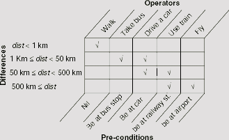
Fig. 11.60. The difference-operator-precondition table.
Table 11.5 Trace of recursive application of means-ends analysis
Difference |
Applicable operator |
Precondition to be satisfied |
|---|---|---|
500 ≤ dist |
fly |
be at airport |
1 ≤ dist < 50 |
drive a car |
be at car |
dist < 1 |
walk (to car) |
nil |
dist < 1 |
walk (to airport) |
nil |
1 ≤ dist < 50 |
take bus |
be at bus stop |
dist < 1 |
walk (to bus) |
nil |
dist < 1 |
walk (to friend’s house) |
nil |
plan generated
walk (to car) → drive (to airport) → walk (to aeroplane) → fly (to ND airport) → walk (to bus stop) → take bus → walk (to friend’s house)
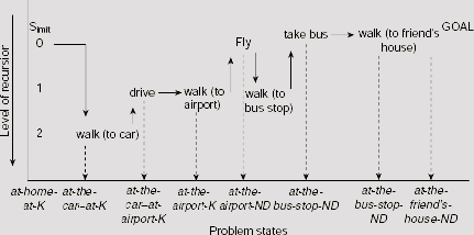
Fig. 11.61. Plan generated through means-end analysis.
11.4.7 Mini-Max Search
Mini-Max search is an interesting type of search technique suitable for game playing AI systems. A game, unless it is one-player puzzle-like, is a typically multi-agent environment in which the agents are competitive rather than cooperative. Each player tries to win the game and makes his moves so as to maximize his chance of win and conversely, minimize the chance of the opponent’s win. As the players have conflicting goals, a player must take into account the possible moves of his opponent while he makes his won move against his opponent. For this reason a search algorithm employed to facilitate decision making for such a player is occasionally referred to as an adversarial search.
In this text, we shall consider only deterministic, two-player, turn-taking, zero-sum games. Such a game can be characterized as follows:
- There are two players. One of them is referred to as the MAX player (say, you), and the other as the MIN player (your opponent). The reason of such nomenclature of the players will be soon obvious.
- The first move is made by the MAX player.
- The moves are deterministic.
- The two players make their moves alternately.
A deterministic, two-player, turn-taking, zero-sum game as described above can be formalized as a system consisting of certain components:
- A data structure to represent the status of the game at any moment. This is usually referred to as the board position. Each possible status of the game is considered as a state of the corresponding state space. The status of the game before the first move (by MAX) is the initial state.
- A successor function which returns a list of legal moves from a given game state as well as the states resultant of those legal moves.
- A terminal condition that defines the termination of the game. Depending on the rules of the game, it may terminate either in the win of a player (and the loss of his opponent), or a draw.
- A function, generally termed as the utility, or objective, or pay-off, or static evaluation function. This function gives the numeric values of the terminal states. In case of static evaluation function, it returns a numeric value for each state of the game. Usually, a positive numeric value indicates a game status favourable to the MAX player and a negative value indicates the game status to be favourable to the MIN player. For example, a winning position for the MAX (MIN) player may have a +∞ (–∞), or +1 (−1) value.
As mentioned earlier, each time a player makes a move he has to consider its impact on his chance of winning the game. This is possible only when he takes into consideration the possible moves of his opponent. Starting with the first move, the entire set of sequences of possible moves of a game can be presented with the help of a game tree. In an ideal situation, a player should be able to identify the perfect move at any turn with the help of the game tree. Example 11.10 illustrates the use of a game tree as an aid to decision making in game playing.
Example 11.10 (The game of NIM)
The game of NIM is a classical example of a deterministic, two-player, turn-taking, zero-sum game. The game starts with a number of piles of sticks. Two players remove sticks from the piles alternately until all the sticks are removed. A player can remove any number of sticks from one pile of his choice when his turn of move comes. However, he should try to leave some sticks in the piles because the player who has to take the last stick loses. The status of the game at any moment may be represented with the help of a non-decreasing sequence of integers. For example, the sequence (2, 4, 4, 7) represents four piles of sticks containing 2, 4, 4, and 7 sticks in the individual piles. Now if a player removes two sticks from one pile containing 4 sticks then the resultant game status is represented by (2, 2, 4, 7). If in this situation all the sticks from the 7-stick pile are removed by a player then the game status becomes (2, 2, 4).
For the sake of simplicity, we shall consider the (1, 2, 2) NIM game. As usual the two players are denoted as the MAX (i.e., you) and the MIN (i.e., your opponent). The utility function is defined as follows:
Function Value |
Interpreatation |
|
|---|---|---|
Won |
Lost |
|
+ ∞ |
MAX |
MIN |
– ∞ |
MIN |
MAX |
It should be noted that instead of the pair (+∞, –∞) other numeric values, e.g., (+1, −1), could also be used. However we shall see that the concept of a utility function will be generalized to that of a static evaluation function which returns an integral value for any game status and not for the winning/losing positions only. The complete game tree for (1, 2, 2) NIM is shown in Fig. 11.62.
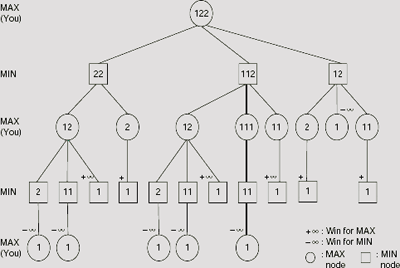
Fig. 11.62. Complete game tree for (1, 2, 2) NIM game.
The root node represents the initial status (1, 2, 2) of the game. Depending on whether the MAX player picks 1 or 2 sticks, the status of the game after the first move may be (2, 2), (1, 1, 2), or (1, 2). These constitute the 1st level nodes of the tree. Similarly, from (2, 2), the move by MIN player may result in the status of (1, 2), or (2), and so on. Usually the set of all game status at a certain level of the game tree which corresponds to the MAX (MIN) player’s turn of move is called a MAX-ply (MIN-ply). To make the distinction clear, nodes of the MAX-ply are represented with circles and those of the MIN-ply are represented with rectangles.
Each leaf node of Fig. 11.62 represents the game status (1), i.e., the last stick. This implies defeat of the player whose turn of move it is. Hence, leaf nodes of a MAX-ply have a utility value –∞ and those of MIN-plies have a value +∞.
The game tree shown in Fig. 11.62 depicts the sequences of probable moves by the two players and the final outcome of those sequences with respect to the result of the game. However, the primary objective of a player is to identify and select the best possible move. The game tree, along with the utility function, may be exploited to achieve this goal.
The idea is to find the utility value, referred to as the Mini-Max value, of each node to decide whether the corresponding move is good or bad for the player. The underlying assumption is that each player will try to create situations best for him and worst for his opponent. Consider the MAX nodes (j) and (k) in Fig. 11.63, which show the game tree of Fig. 11.62 along with the Mini-Max values of the nodes. Nodes (j) and (k) are losing the game status for MAX. Therefore, both of them have a score of −∞. Now node (j) is a child of node (g) which is a MIN node. Since MIN will definitely try to defeat MAX, it is bound to make a move that leads to game status (j). Hence the utility value of (g) is same as that of (j). Similarly, the utility of node (k) is propagated to node (h). However, node (i) of the same MIN-ply is a losing game status for a player MIN and a win for node MAX. Hence its score is +∞. Now (g), (h) and (i) are children of node (e), which belongs to a MAX-ply. MAX will select a move to ensure his chance of win. Among (g), (h) and (i), the first two imply defeat of MAX and the last one ensures his win. Therefore, faced with situation (e) MAX will make a move to (i) only, neither (g) nor (h). Hence the Mini-Max value of node (e) should be same as that of (i), i.e., +∞. However, the situation is reverse for the node (c). This node has three children with Mini-Max values +∞, −∞, and +∞, respectively. Being in a MIN-ply, the opponent will try to make things worst for MAX and so will move to the game status of value −∞. Hence the Mini-Max value of (c) is −∞. Obviously, the general rule for computing the Mini-Max value of a node N is:
- If N is a leaf node then the Mini-Max value of N is its score, i.e., value of the utility function at that node.
- If N is a MAX-node, i.e., N belongs to a MAX-ply, the Mini-Max value of N is the maximum of the Mini-Max values of its children.
- If N is a MIN-node, i.e., N belongs to a MIN-ply, the Mini-Max value of N is the minimum of the Mini-Max values of its children.
Procedure MiniMax (N) (Fig. 11.64) gives the pseudo-code for the technique mentioned above. In case of a MAX node, the Mini-Max value is initialized to −∞ (or the minimum allowable value) and then gradually updated to the maximum value of its children. (lines 3-9). For a MIN node the value is initialized to +∞ and then lowered down to the minimum value among its children. Fig 11.63 shows the Mini-Max values of each node of the game tree for (1, 2, 2) NIM game obtained by applying this procedure on the said game tree. It is easy to see that the root node attains a Mini-Max value of +∞ which implies that if properly played, the game can be won by the MAX player and in order to win he has to remove the stick from the single stick pile. Any other move may eventually lead to his losing the game, provided the opponent does not make any mistake.
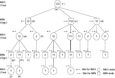
Fig. 11.63. Utility values of different nodes of (1, 2, 2) NIM game.
A realistic game playing system must take into consideration the facts that the real-world games are too hard computationally. As a classical example, consider the game of chess. The average branching factor of chess is approximately 35. If we consider a usual game with 50 moves for each player then the search tree would consist of about 35100 or 10154 nodes. Arriving at an optimal decision through exhaustive search of a tree of such dimension is not feasible. Hence Procedure MiniMax (N) has to be modified suitably so that effective decisions can be taken even if the entire game tree is not searched.
Static evaluator We need something more than a utility function to assist us in decision making while playing a realistic game. Recall that the utility function returned a value for terminal game status, which is percolated to their ancestors as Mini-Max values till the concerned node attains its own MiniMax value. A static evaluator is a generalized utility function that returns a value for any node of the game tree and not just for the terminal modes. Equipped with a suitable static evaluator Procedure MiniMax (N) can now be modified to carry out the Mini-Max search to a predefined depth from the given node of the game tree and assign the Mini-Max value of the node on the basis of that limited information.
Procedure MiniMax (N) |
|
|
INPUT :A node N of a game tree TG. Also there is an evaluation function score(N) which returns a value indicating the relative merit of the game status corresponding to node N. Usually score(N) = –∞ if N is a winning position for MIN, and score(N) = +∞ if N is a winning position for MAX. |
|
OUTPUT: The MiniMax value of node N. |
1. |
BEGIN |
2. |
IF (N is a leaf node) THEN Return score(N) END-If |
|
/* code for MAX node */ |
3. |
IF (N is a MAX node) THEN |
|
/* Initialize MiniMax value with lowest possible value */ |
4. |
MiniMax-value ← –∞ |
|
/* Update the MiniMax value of the current node with the highest |
|
MiniMax value among its children */ |
5. |
FOR (each child of N) DO |
6. |
value ← MiniMax (child) |
7. |
IF value > MiniMax-value THEN MiniMax-value ← value END-If |
8. |
END-For |
9. |
Return MiniMax-value |
10. |
END-If |
|
/* code for MIN node */ |
11. |
IF (N is a MIN node) THEN |
|
/* Initialize MiniMax value with highest possible value */ |
12. |
MiniMax-value ← +∞ |
|
/* Update the MiniMax value of the current node with the lowest MiniMax value among its children */ |
13. |
FOR (each child of N) DO |
14. |
value ← MiniMax (child) |
15. |
IF value < MiniMax-value THEN MiniMax-value ← value END-If |
16. |
END-For |
17. |
Return MiniMax-value |
18. |
END-If |
19. |
END-MiniMax |
Fig. 11.64. Procedure MiniMax (N).
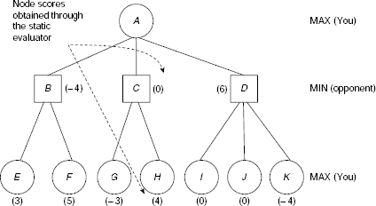
Fig. 11.65. Scores of individual nodes based on static evaluation function.
Depth-limited Mini-Max search As an example, let us consider a portion of an imaginary game tree as shown in Fig. 11.65. The score of each node with respect to the evaluation function is given within parentheses adjacent to the respective node. Our goal is to assign a Mini-Max value to the root node A on the basis of these scores. If we decide to carry out the Mini-Max search process till a depth of 1 only, then the scores of three children of A, i.e., nodes B, C and D, should be considered and no node beyond that level. As A is a MAX node, the maximum of these scores should be the Mini-Max value of A (see Fig. 11.66). Therefore node A attains a Mini-Max value of 6 through 1-ply MiniMax search.
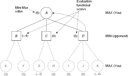
Fig. 11.66. Finding Mini-Max value through 1-ply search.
Now compare this with Fig. 11.67 showing the same process carried out to a depth of 2, instead of 1. Here the deepest nodes are at level 2 and these nodes are evaluated on the basis of the static evaluator. The nodes B, C and D being MIN nodes, each of them obtain its Mini-Max value as the lowest score among the children of the respective node. Finally, the MAX node A is assigned a Mini-Max value of 3, the highest score among B, C and D.
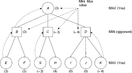
Fig. 11.67. Finding Mini-Max value through 2-ply search.
The pseudo-code for the technique described above is presented in Procedure Depth-Limited-MiniMax (N, d) (Fig. 11.68). The algorithm is similar to MiniMax (N) except that each time the procedure calls itself recursively the depth is reduced by 1. Therefore, score (N) is returned not only for the leaf nodes but also for the nodes at depth d (line #2).
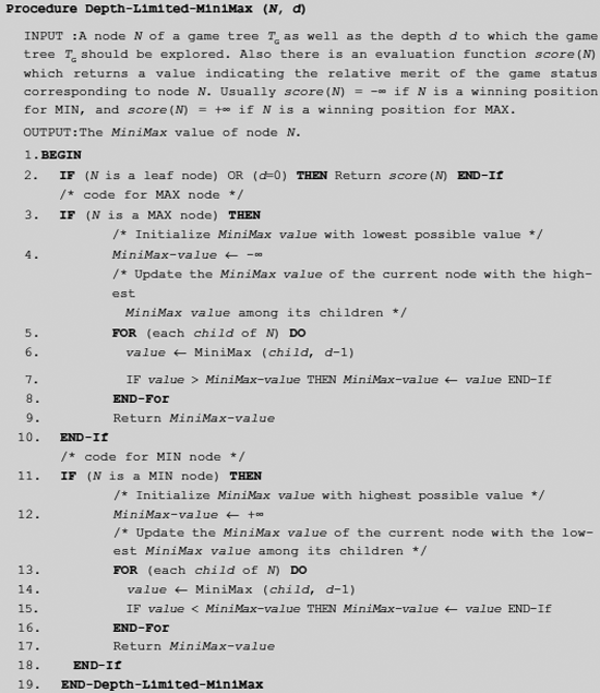
Fig. 11.68 Procedure depth-limited-MiniMax (N, d).
Design issues While designing a game playing system using Mini-Max search, one has to decide two things, viz., which static evaluator is to be employed, and how deeply the game tree should be searched. There is no rule regarding the first issue. It depends on the insight of the designer. However, several factors are to be taken into consideration in this regard. Most important of these are
- Speed: The static evaluator should compute fast. This is because time is a decisive parameter in most of the games we humans play. For example, in chess any delay in making a move is eventually severely punished.
- Heuristic power: The static evaluator should be powerful enough to embody sufficient knowledge regarding the game so that effective decision can be taken by the player. Again, let us consider the game of chess. A simple static evaluator would be the sum of the values of the white pieces minus the sum of the values of the black pieces, i.e.,
where pW and pB are the white pieces and the black pieces remaining in board position N.
The question of how deeply should the game tree be searched is related to the speed-concern as well as the heuristic power of the static evaluator. The deeper we delve into the game tree the more informed and wise our decision, provided we have time. We may also try to compensate, so far as possible, the limitation of the evaluator by carrying out the search to deeper levels.
Alpha-beta pruning Is it possible to make MiniMax search more efficient? It has been found quite frequently that certain portions of a game tree do not play any role to decision-making in the sense that the Mini-Max value returned by the search remains the same irrespective of whether these portions are explored or not. Alpha-Beta pruning is a technique of making MiniMax search efficient by avoiding these parts while searching the game tree. The technique of Alpha-Beta pruning is explained below with reference to the game tree shown in Fig. 11.69.
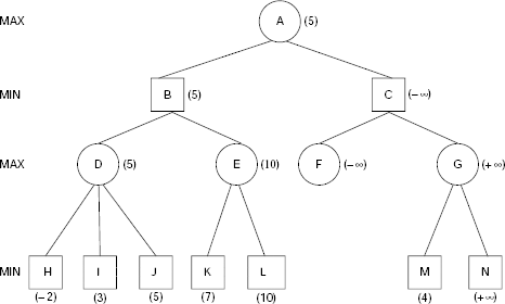
Fig. 11.69. A 3-ply game tree with Mini-Max values.
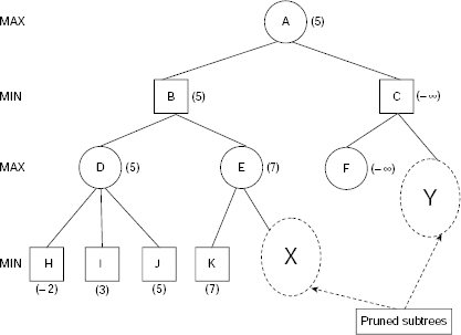
Fig. 11.70. Alpha-Beta pruning of a game tree during Mini-Max search.
As usual, the numbers attached to the leaf nodes are the scores of the respective game status obtained through the static evaluator and the numbers adjacent to the internal nodes give the Mini-Max values. The root node A obtains a Mini-Max value of 5 as a result of 3-ply Mini-Max search on the game tree mentioned above. Let us examine the Mini-Max process involved here critically. The MAX node D is assigned a MiniMax value 5 as this is the highest score among its children H, I and J. Now, while computing the Mini-Max value of node E, we see that E’s first child K has a score of 7. This implies the Mini-Max value of E is going to be at least 7, as E is a MAX node. But this value is already greater that 5, the Mini-Max value of node D. Since the parent of D and E, i.e., node B, is a MIN node, the Mini-Max value of B will be at most 5. Hence it is useless to explore the sub-tree marked ‘X’ (see Fig. 11.70). Whatever be the values existing in portion ‘X’ of the game tree, the Mini-Max value of B will remain 5. Similarly, the ‘Y’ portion of the game tree can also be ignored because the MIN node C has already attained a Mini-Max value -∞ which obviously can not be further lowered.
Procedure AlphaBeta-MiniMax (N, d, Alpha, Beta) (Fig. 11.71) presents the pseudo-code for MiniMax search made efficient by incorporating the technique of Alpha-Beta pruning explained above. Alpha and Beta are the two cutoff numbers, generally referred to as the Alpha-Beta cut-offs, used to prune the avoidable parts of the game tree. The Mini-Max value of node is worth computing only if it lies within the range [Alpha, Beta]. While computing the Mini-Max value of a MAX node as soon as it is found that the Mini-Max value of any of its child exceeds Beta then the concerned MAX node is assigned a value of Beta without exploring the rest of the subtree (see line #8 of Procedure AlphaBeta-MiniMax). Conversely, a MIN node is assigned the Mini-Max value Alpha as soon as it tends to go below Alpha, and the search is discontinued (see line #17 of Procedure AlphaBeta-MiniMax). A trace of execution of Procedure AlphaBeta-MiniMax on the game tree of Fig. 11.69 is shown in Table 11.6. The recursive calls of Procedure AlphaBeta-MiniMax (N, d, Alpha, Beta) are underlined. A pictorial view of the process is presented in Fig. 11.72.
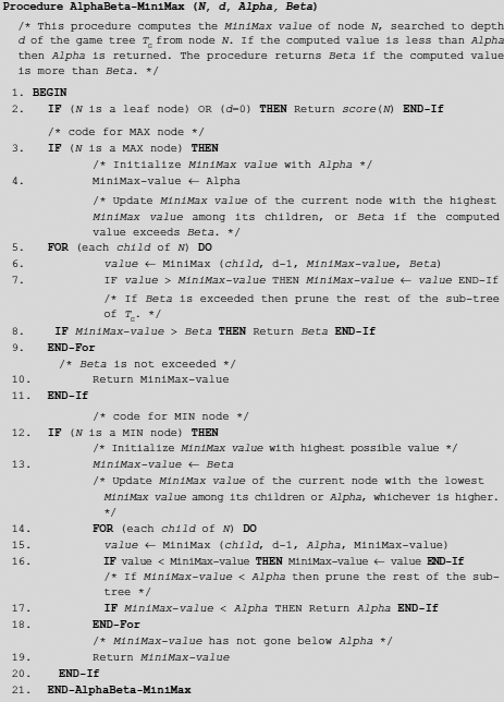
Fig. 11.71. Procedure AlphaBeta-MiniMax (N, d, Alpha, Beta).
Table 11.6. Trace of execution of procedure AlphaBeta-MiniMax
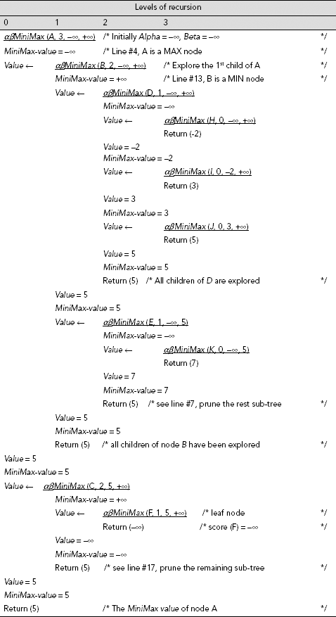
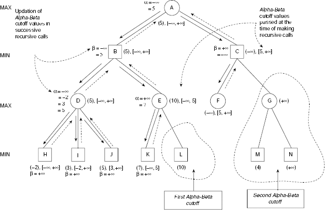
Fig. 11.72. Alpha-Beta pruning during MiniMax search.
The effectiveness of Alpha-Beta pruning depends on the order in which the nodes are visited. For a MAX node, the best case is exploration of the best child (best from the point of view of MAX player) first so that remaining children and sub-trees associated with them becomes irrelevant. On the other hand, visiting the worst child (worst from the point of view of MIN) is most welcome in case the concerned node is a MIN node. These correspond to pruning to the highest extent. However, there may be no pruning at all if the children are visited in the worst order.
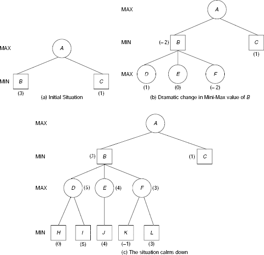
Fig. 11.73. Waiting for quiescence.
Quiescence How deep should we delve into the game tree while performing the depth-limited Mini-Max procedure on it? The problem is, a seemingly good move at a certain level may turn out to be a bad one, or vice versa, if the game tree is searched further. Take, for example, the situation depicted in Fig. 11.73(a), (b), and (c). Fig. 11.73(a) shows the beginning of search for the Mini-Max value of node A. The nodes B and C are at level 1 and they have scores 3 and 1, respectively. Therefore, on the basis of the search till depth 1, the Mini-Max value of A should be max (3, 1) = 3. The situation dramatically changes when the game tree is explored one level deeper (see Fig. 11.73(b)). What was thought to be a good move represented by the node B, now appears as a very bad one because this gives the opponent an opportunity to worsen the condition of MAX player. However, if we go one level deeper into the game tree, as depicted in Fig. 11.73(c), we see that the node B regains its previous Mini-Max value and seems to be a good choice for MAX as earlier.
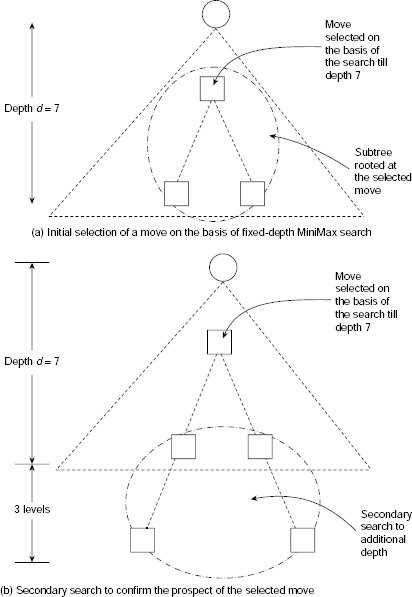
Fig. 11.74. Secondary search to neutralize horizon effect.
The fact is, short-term measures occasionally influence our choice of move adversely and it is not wise to take a decision without considering the long-term effects. To achieve wise selection of a move among a number of alternatives, one should go on exploring the game tree deep enough to reach a stable condition. The stable condition is recognized when it is found that no drastic change occurs from one level to the next. This strategy for determination of the appropriate depth to which depth-limited Mini-Max search is to be conducted is known as waiting for quiescence. The quiescence problems are difficult to eliminate altogether. One such example is the so-called horizon effect. It appears when a player is facing a move by the opponent which is bad for him but inevitable in the long run. A fixed-depth Mini-Max search may try to avoid such a fatal move by using some tactics, say a move that keeps the opponent busy for the time being. But such tactics only push the fatal move to the search horizon and merely delay the inevitable blow.
Secondary search Is there any way to tackle the horizon effect? A technique called secondary search is found to be helpful in this regard. Essentially, it consists of searching a portion of the game tree, not the entire game tree, for a few additional levels. Let us suppose that the game tree is searched to an average depth of, say seven. Let a move N be primarily selected on the basis of this search. In order to ensure that N is really a good move we may further explore the sub-tree rooted at N for additional three levels. But this additional search is not performed on any other portion of the game tree. This is called secondary search. Fig. 11.74 illustrates the technique pictorially.
Book moves In general, whenever a player has to make a move during a game, he faces a lot of alternatives among which the best, according to his own strategy of playing, is to be identified and applied. MiniMax search, empowered with appropriate heuristic knowledge, is employed to achieve this. A kind of heuristic search is practically indispensable because the other alternative is to build a catalogue of best moves corresponding to every conceivable game status and extract it during the game through a table look-up procedure. This is simply not feasible considering the immensity of the search space.
However, selective use of such moves, usually referred to as book moves, do enhance the performance of the program. For example, the opening and endgame sequences of chess are highly stylized. One may reasonably maintain a list of moves relevant to these parts of the game and use them directly without groping for a suitable move within the game tree through Mini-Max search. A judicious combination of book moves during the opening sequence, endgames, and Mini-Max search procedure for the midgame, would enable the program to attain a level of efficiency which neither book moves nor search alone could achieve.
11.4.8 Constraint Satisfaction
Quite often we encounter a problem in AI that can be modeled as a constraint satisfaction problem (CSP). Here the goal is to reach a state that satisfies certain restrictive conditions, or constraints, among the parameters of the problem. As a typical CSP, we may think of the famous graph colouring problem, also referred to as map colouring problem. An instance of this problem is shown in Fig. 11.75(a). It shows an area divided into six regions A, B, C, D, E and F. The regions are to be coloured with red, blue, or yellow in such a way that no two adjacent regions may have the same colour. Here the problem may be viewed as that of assigning certain values to six variables A, B, C, D, E and F, the values must be taken from the set {red, blue, yellow}, such that if X and Y are adjacent regions in the map, i.e., X, Y ∈ {A, B, C, D, E, F}, X ≠ Y, then v(X) ≠ v(Y), where v(X) and v(Y) are the values, i.e., colours, assigned to X and Y, respectively.
The adjacency relationships among these six regions are depicted as an undirected graph in Fig. 11.75(b). Each node of the adjacency graph represents a region of the map. If two regions X and Y are adjacent in the map then there is an edge in the adjacency graph between the nodes corresponding to these regions. The adjacency graph for a given map colouring problem is also its constraint graph in the sense that it represents the constraints regarding the colours of the regions. An edge between two nodes P and Q of a constraint graph indicates that the regions corresponding to P and Q should have different colours.
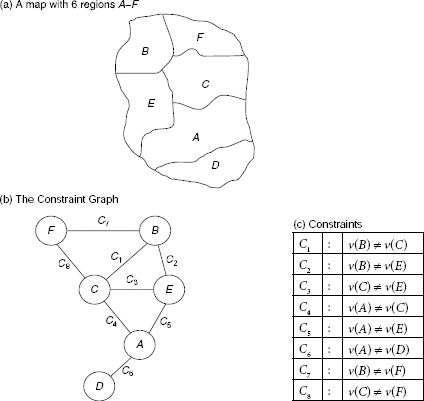
Fig. 11.75. (a)–(c). Map coloring as a constraint satisfaction problem.
A Constraint Satisfaction Problem (CSP) is defined by the following features:
- A set of variables, X1, X2,…, Xn.
- For each variable Xi a non-empty domain D(Xi) of possible values of Xi.
- A set of constraints, C1, C2, …, Cm. Each constraint Ci involves some variables Xp, Xq … etc. and a specification of the allowable combination of values for these variables.
The map coloring problem presented in Fig. 11.75 can now be formulated as a CSP in the following way:
CSP Formulation of graph colouring problem
1. |
Variables |
A, B, C, D, E, F |
2. |
Domains |
DA = DB = DC = DD = DE = DF = {red, blue, yellow} = { R, B, Y} |
3. |
Constraints |
C1’:v (B) ≠ v (C) ≠ v (E) |
C2’:v (A) ≠ v (C) ≠ v (E) |
||
C3’:v (B) ≠ v (C) ≠ v (F) |
||
C4’:v (A) ≠ v (D) |
It should be noted that there are only four constraints in the CSP formulation given above even though eight constraints are depicted in Fig. 24.1(c). This is because each of the constraints C1, C2,…, C8 of Fig. 11.75(c) involves only two variables whereas the constrains C1′, C2′, C3′ involve three variables each. So effectively C1′, C2′, C3′ taken together consolidates all the constraints C1 through C8. In fact, in CSPs we encounter three kinds of constraints, viz., unary constraints, binary constraints, and general constraints.
A constraint that involves just one variable is termed as a unary constraint. A binary constraint involves two variables and constraints involving more that two variables are called general constraints. Each of the constraints C1, C2,…, C8 of Fig. 11.75(c) is a binary constraint. Constraints C1’, C2’, C3’ are general constraints. There is no unary constraint in the map colouring problem stated above. However, a constraint like v(A) ≠ red exemplifies the category of unary constraints. A general constraint can always be broken down to an equivalent set of binary constraints.
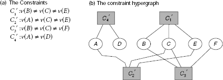
Fig. 11.76. General constraints and constraint hypergraph.
A constraint hypergraph is a graphical structure that represents the constraints involving the variables. For each variable of the given CSP there is a distinct node in the corresponding constraint hypergrah. A constraint C(X1, X2, …, Xk) involving k variables is represented by a hyperedge among the nodes X1, X2, …, Xk. When all constraints are binary the corresponding constraint hypergraph becomes a constraint graph, as shown in Fig. 11.75(b). Fig. 11.76 shows the constraint hypergraph for the map colouring problem discussed above.
An assignment S for a given CSP, represented as S = {〈Xp, vp〉, 〈Xq, vq〉, … 〈Xr, vr〉}, is an attachment of some legitimate values, say vp, vq, … vr to some or all variables Xp, Xq, …, Xr such that vp∈ D(Xp), vq∈ D(Xq), …, vr∈ D(Xr). If none of the variables are assigned any value then it is said to be an empty assignment. For the map colouring problem shown in Fig. 11.75, S = {〈A, blue〉, 〈B, yellow〉, 〈C, yellow〉, 〈D, red〉, 〈E, blue〉, 〈F, red〉} is an assignment.
If an assignment does not violate any constraint then it is said to be consistent or legal assignment. The assignment stated above, i.e., S1 = {〈B, yellow〉, 〈C, yellow〉, 〈E, blue〉, 〈F, red〉} is not consistent because it violates the first constraint v (B) ≠ v (c). However, it can be easily seen that S2 = {〈A, blue〉, 〈B, blue〉, 〈C, yellow〉, 〈D, red〉, 〈E, red〉, 〈F, red〉} is a consistent assignment.
An assignment in which all the variables are attributed some value is said to be a complete assignment. For example, assignment S2 cited above is complete, though S1 is not a complete assignment.
Finally, a solution to a given CSP is a complete assignment that satisfies all the constraints. The assignment S2 cited above is complete, and it satisfies all the constraints C1, C2,…, C8. Therefore S2 is a solution to the given map colouring problem. In some CSPs, along with the basic requirement of satisfying all the constraints, there is an additional requirement of optimizing a pre-defined objective function.
Solving constraint satisfaction problems Once a problem is formulated as a CSP, any suitable search procedure can be employed to find a solution. Given a CSP, the suitability of a search procedure as a solution strategy is judged by the characteristics of the CSP concerned. However, two widely accepted strategies are frequently employed, viz., backtracking depth-first search (BDFS), and min-conflict local search. Each of these are explained below with appropriate examples.
Backtracking depth-first search (BDFS) Consider the map coloring problem presented in Fig. 11.75 and later formulated as a CSP. A backtracking DFS would start with the empty assignment {} which corresponds to the initial state of the search space. Let us suppose that assignment of colour to the regions of the map will be made in the sequence A, B, C, D, E, and F. Since the domain DA = {red, blue, yellow} = ![]() the region A may be assigned the color red, blue, or yellow, so that we may attain any one of the assignments, or problem states, 〈A, red〉, 〈A, blue〈, 〈A, yellow〉, or
the region A may be assigned the color red, blue, or yellow, so that we may attain any one of the assignments, or problem states, 〈A, red〉, 〈A, blue〈, 〈A, yellow〉, or ![]() . These constitute the children of the root node {} of the search tree, shown in Fig. 11.77. Each node of Fig. 11.77 represents an assignment obtained by concatenating the individual assignments along the path from the root to that node. For example node 2 corresponds to the assignment
. These constitute the children of the root node {} of the search tree, shown in Fig. 11.77. Each node of Fig. 11.77 represents an assignment obtained by concatenating the individual assignments along the path from the root to that node. For example node 2 corresponds to the assignment ![]() , and node 5 represents the assignment
, and node 5 represents the assignment ![]() . Let us choose, arbitrarily, the assignment {〈A, red〉} among the three alternatives and proceed to assign a colour to the region B.
. Let us choose, arbitrarily, the assignment {〈A, red〉} among the three alternatives and proceed to assign a colour to the region B.
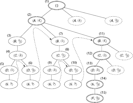
Fig. 11.77. Backtracking depth-first search for the map colouring problem.
As A and B are not adjacent regions the colour of A does not affect the choice of the colour of region B. Therefore, B can be assigned any of the values ![]() and accordingly three children of node (2) are created, viz.,
and accordingly three children of node (2) are created, viz., ![]() (node (3)),
(node (3)), ![]() (node (7)), and
(node (7)), and ![]() (node (11)). The nodes of the search tree of Fig. 24.3 are numbered according to the order of exploration. Again, we arbitrarily select
(node (11)). The nodes of the search tree of Fig. 24.3 are numbered according to the order of exploration. Again, we arbitrarily select ![]() for further exploration. The candidate for assignment of color is now region C. Since C is adjacent to both A and B, its colour has to be different from that of A and B, i.e., red and yellow. Therefore the only choice left for region C is blue (node (4)). Next it is D’s turn. D is adjacent to A only and A has already been assigned red. Obviously, D may either be blue or yellow (see nodes (5) and (6) of Fig. 11.77). We proceed along node (5). Now when we try to assign a colour to E we see that as it is adjacent to A, B, and C and A, B, and C have the colours red, yellow and blue, there is no colour left for E. So we backtrack and explore node (6). But the situation does not change. Once again we back track and select another child of node (2), i.e., node (7).
for further exploration. The candidate for assignment of color is now region C. Since C is adjacent to both A and B, its colour has to be different from that of A and B, i.e., red and yellow. Therefore the only choice left for region C is blue (node (4)). Next it is D’s turn. D is adjacent to A only and A has already been assigned red. Obviously, D may either be blue or yellow (see nodes (5) and (6) of Fig. 11.77). We proceed along node (5). Now when we try to assign a colour to E we see that as it is adjacent to A, B, and C and A, B, and C have the colours red, yellow and blue, there is no colour left for E. So we backtrack and explore node (6). But the situation does not change. Once again we back track and select another child of node (2), i.e., node (7).
The backtracking depth-first search proceeds in this way until it finds a complete assignment that satisfies all the constraints. In Fig. 11.77 this complete assignment is obtained by concatenating the individual assignments of nodes 1, 2, 11, 12, 13, 14, and 15 and is given by ![]() . The arrows in Fig. 11.77 show the backtracking paths.
. The arrows in Fig. 11.77 show the backtracking paths.
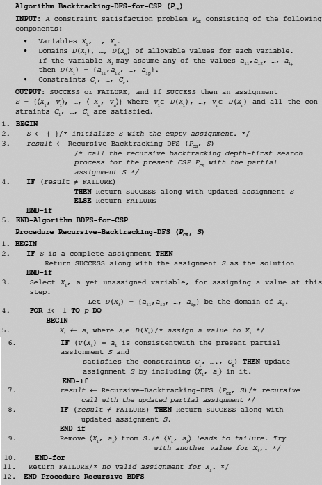
Fig. 11.78. Algorithm backtracking-DFS-for-CSP (Pcs)
Algorithm Backtracking-DFS-for-CSP (PCS) (Fig. 11.78) presents the pseudocode for the basic strategy of backtracking depth-first search for solving CSPs. The algorithm starts with empty assignment {} and progressively assign values to the variables and makes recursive calls so that if any assignment leads to inconsistency, or hinders subsequent assignments, then it may backtrack and try with some other value.
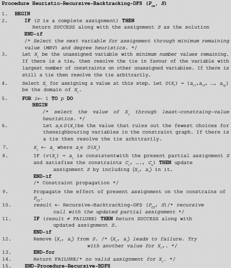
Fig. 11.79. Procedure heuristic-recursive-backtracking-DFS (Pcs, S)
Heuristics Algorithm Backtracking-DFS-for-CSP described above is a simplified version of the actual procedure followed in practice. It does not consider how to make the selection when choices are there. For example
- In step 3 of Procedure Recursive-Backtracking-DFS (PCS, S) a variable is to be selected from the set of unassigned variables for the purpose of assigning a value. The criteria underlying this selection are not stated.
- Step 5 of the same procedure assigns a value to the current variable. It is not clearly stated how to select an appropriate value from the corresponding domain which, in general, should contain several legal candidate values.
- What are the implications of an assignment on the remaining unassigned variables and how to reduce the search space so that the process of legal assignment to variables is made efficient?
Regarding points 1 and 2 above, there are heuristics to facilitate selection of a variable for the purpose of value assignment as well as selection of a value to be assigned. Similarly, strategies to propagate the effect of a certain assignment to other variables are also there. Procedure Heuristic-Recursive-Backtracking-DFS (PCS, S) (Fig. 11.79) shows the procedure after incorporation of the heuristics discussed below.
Minimum remaining value (MRV) and degree heuristic According to minimum remaining value (MRV) heuristics the variable with least number of legal values still available for assignment is to be selected for next assignment. For example, consider the assignment {〈A, blue〉, 〈E, red〉, 〈F, red〉}. Considering the constraints, this assignment leaves the domains of the remaining variables as DB = {blue, yellow}, DC = {yellow} DD = {red, yellow}. As the region C has the least number of remaining legal values, according to the MRV heuristics, this will be selected for the next assignment.
However, MRV heuristics may not help initially because then all the variables have their domains in full capacity, or in case two or more variables have the same minimal number of remaining variables. To resolve such situation the degree heuristics may be employed. The degree heuristics selects the variable that is involved in the largest number of constraints on other unassigned variables. For example, consider the map colouring problem stated above. Initially all the variables have the same domain {red, blue, yellow} which renders the MRV heuristic ineffective. However, it is seen from the constraint graph (Fig. 11.75(b)) that region C is involved with four regions A, B, E and F through constraints which is the highest among all the variables. Hence, applying the degree heuristic we choose C as the first variable to be assigned a value.
Least constraining value Once a variable is chosen, it is required to assign a legal value from its current domain. Since the domains normally contain several candidates the issue of selecting the most desirable value becomes relevant. Here the least constraining value heuristic is helpful. According to this heuristic, the value which rules out least number of candidates from the domains of the neighbouring variables is preferred. For example, suppose that at an instant the domains of F and B are DF = {red, yellow} and DB = {yellow} and it is F’s turn to be assigned a value. If we assign yellow then it is removed from the domain of B, making DB = {}. However, if red then DB remains non-empty and it is feasible for region B to get a legal value. Therefore, the value red is less constraing than yellow and B should be assigned the value red instead of yellow.
Table 11.7. Trace of Procedure heuristic-recursive-backtracking-DFS for map colouring problem of Fig. 11.75
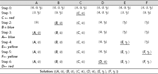
Forward chaining and constraint propagation Assignment of a value to a variable obviously has its effects on the domains of the remaining variables. Constraint propagation is the process of propagating the implications of a constraint on the variables onto the other variables. Suppose, as an example, that in the first step of the map colouring problem, the region C has been assigned the value red. Since A, B, E and F are all involved with C through the constraints C4, C1, C3, and C8, respectively, the domains of all these variables reduces to {blue, yellow}. However, the domain of D remains {red, blue, yellow} as it is not involved with C through any constraint. This procedure, which, after an assignment is made, modifies the domains of the unassigned variables so that the modified domains are consistent with the assignment, is called forward checking. However, mere forward checking is not sufficient. Suppose, after assigning red to C, we assign blue to E. This will reduce the domain of A to {yellow} as A is adjacent to E. Moreover, since D is associated with A through the constraint C6, the domain of D is in turn reduced from {red, blue, yellow} to {red, blue}. In this way the effect of a certain assignment is propagated to other unassigned variables through forward checking followed by further modification of the domains so that the values attain consistency with respect to the constraints.
The entire process can be illustrated with reference to the graph colouring problem. A trace of the progress of the algorithm is shown in Table 11.7 and the stepwise description is provided below.
Step 0. |
We start with the empty assignment {}. All the variables have the same domain {red, blue, yellow}, abbreviated as |
Step 1. |
We have to select a variable for assignment. Since all domains have the same number of values the MRV heuristic is not applicable. Therefore, the degree heuristic is to be followed. Consulting the constraint graph (Fig. 11.75(b)), it is found that C is involved with the maximum number of variables, 4 in this case, through constraints. Hence C is chosen for assigning a value. We make the assignment C ← red and propagate the effect of this assignment on other variables. As a result of this propagation all the variables involved with C through constraints, i.e., A, B, E and F, remove red from their domains. However, the domain of D remains unchanged because it is not adjacent to A. The state of the problem after step 1 is |
Step 2. |
Applying the MRV heuristic we find four candidates A, B, E and F for the next assignment. The number of unassigned variables these are attached to in the constraint graph are 2, 2, 2 and 1, respectively. Again there is a tie among A, B, and E. Let us resolve the tie by arbitrarily choosing B for assignment this time. We make B ← blue, so that the state becomes |
Step 3. |
Now each of A, E and F have just one remaining value in their respective domains. So let us take the help of the degree heuristic to break the tie. A is attached to two of the still unassigned variables, viz., D and E. E is adjacent to only A and F is no more attached to any unassigned variable. Therefore A is the next candidate for value assignment and the only value in its domain, blue, is assigned to it. Now the assignment is |
The subsequent steps, i.e., steps 4, 5, and 6 can be easily worked out and are depicted in Table 11.7. The final assignment is![]() Fig. 11.80 shows the solution tree corresponding to the heuristic recursive backtracking depth-first search described above.
Fig. 11.80 shows the solution tree corresponding to the heuristic recursive backtracking depth-first search described above.
Min-conflict local search The backtracking depth-first search strategy described above for solving a CSP starts with the empty assignment {} and incrementally proceeds to a complete assignment consistent with the constraints. An alternative approach is to start with a complete assignment, perhaps arbitrarily generated, and then employ some local search procedure which transforms this complete but non-solution assignment onto a complete and consistent assignment, i.e., a solution. Algorithm Min-Conflict-for-CSP (PCS, MAXsteps) (Fig. 11.81) presents a pseudo-code for the procedure mentioned above. At each iteration, a variable is identified which is under conflict as per the given constraints (line 8). It is then tried with values other than the present one and the value for which the variable suffers minimum amount of conflict is chosen. The current assignment is then modified to that which incorporates this latest value. In this way newer variables are modified over and over again until either we get an assignment which satisfies all constraints and therefore offers a solution, or exceeds a predefined maximum number of iterations. The min-conflict local search process is illustrated with the help of the 8-queen problem which is stated below.
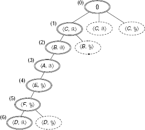
Fig. 11.80. Solution tree corresponding to the heuristic recursive backtracking depth-first search to solve the map colouring CSP.
Example 11.11 (The 8-queen problem)
Is it possible to arrange 8 queens on a chess board in a way such that none of them is in an attacking position with respect to any other?
The generalized form of the 8-queen problem is the n-queen problem, which states that given an n × n array, is it possible to arrange n number of queens within the array in a way such that none of them attack any other and if yes, then to find one such arrangement of the n queens.
Let us denote the eight queens by the variables QA, QB, QC, QD, QE, QF QG, and QH. The queens corresponding to the variables QA, QB, QC, QD, QE, QF QG, and QH are in the columns A, B, …, H, respectively. As no queen is attacking any other all the queens must be in different columns. Let us number the 8 rows as 1, 2, 3, 4, 5, 6, 7, and 8. Then each variable mentioned above may take a value from the set {1, 2, 3, 4, 5, 6, 7, 8}. We are now in a position to formulate the 8-queen problem as a CSP.
CSP formulation of the 8-queen problem
1. |
Variable: |
QA, QB, QC, QD, QE, QF, QG, QH |
2. |
Domains: |
DA = DB = DC= DE = DF = DG = DH |
= {1, 2, 3, 4, 5, 6, 7, 8} |
||
3. |
Constraints: |
For all pairs QX and QY, X,Y ∈ {A, B, C, D, E, F, G, H}, X ≠ Y, QX and QY should be in non-attacking position, i.e. not in the same row, column or diagonal. |
The initial arrangement of the 8 queens is shown in Fig. 11.82 (a). It corresponds to the assignment {〈QA, 8〉, 〈QB 5〉, 〈QC, 1〉, 〈QD, 6〉, 〈QE, 3〉, 〈QF, 7〉, 〈QG, 2〉, 〈QH, 4〉}.
However, this assignment is not consistent with the constraints because the queens at positions 8A and 2G are attacking each other diagonally. Similarly, the queens at 1C and 3E are also attacking each other. At this point we employ the min-conflict local search procedure and look for a better position for the queen presently at the position 8A. With this purpose in mind, for each other position of the queen in column A we find the number of queens in conflict if the current queen is placed in respective cell.
For example, if the queen is placed in cell 4A then it will be attacked by two queens at positions 4H and 5B. Hence the value (2) is associated with the cell 4A. Similarly the other values are found. Now there is a tie regarding the lowest conflict count. Both cells 1A and 5A are having the same minimum value 1. The tie is arbitrarily resolved in favour of cell 1A. The queen concerned is placed at this position so that the assignment after the first becomes {〈QA, 1〉, 〈QB, 5〉, 〈QC, 1〉, 〈QD, 6〉, 〈QE, 3〉, 〈QF, 7〉, 〈QG, 2〉, 〈QH, 4〉} (the change is highlighted with boldfaces). After QA we focus our attention on QB. Fortunately, QB is already in a non-conflicting position with respect to other queens. Therefore, we leave it in the same position and proceed to find a better place for QC which is in conflict with QA and QE (Fig. 11.82(b)). It is found that at cell 8C the queen QC is in non-attacking position. Making this assignment we arrive at the state {〈QA, 1〉, 〈QB, 5〉, 〈QC, 8〉, 〈QD, 6〉, 〈QE, 3〉, 〈QF 7〉, 〈QG, 2〉, 〈QH, 4〉}, which satisfies all the constraints and therefore is a solution to the given problem.
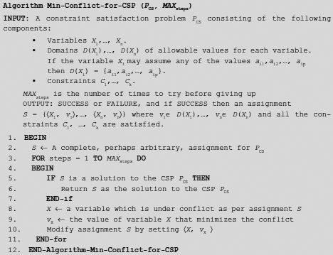
Fig. 11.81. Algorithm Min-Conflict-for-CSP (PCS, MAXsteps).
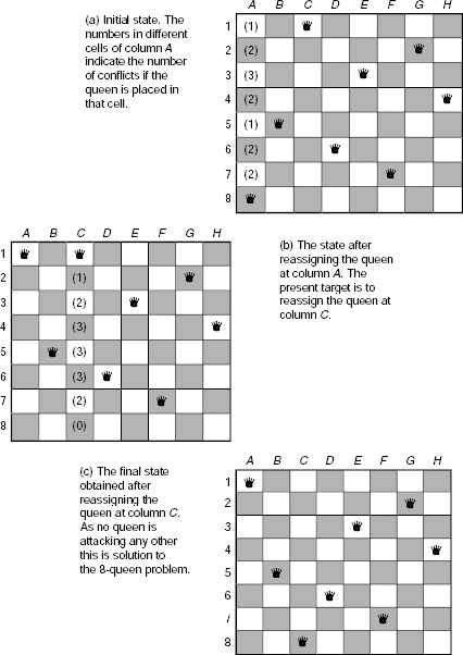
Fig. 11.82. (a)-(c) A min-conflict local search procedure to solve the 8-queen problem
11.4.9 Measures of Search
The efficiency of a heuristic search depends to a large extent on the quality of the heuristic evaluation function employed. Better heuristic results in less computational effort without compromising the success of the search process. However, it is hardly possible to make an estimation of heuristic power through direct calculation because it depends on too many factors.
Instead, certain computable measures of performance are frequently used to compare the performances of various search processes. Two of these are penetrance and effective branching factor.
Penetrance. P of a search process is defined as the ratio of the length of the path from the start state to the goal state reached through the search and the total number of nodes generated during the search, including the goal node but excluding the start node.
Here L is the length of the path from the start state to the goal state, and N is the total number of nodes generated during the search. Penetrance is the measure of how focused the search was towards the goal. In the ideal case, the search process has complete knowledge of the problem, and only those nodes are generated which are on the path from the start node to the goal node. The value of P for such an ideal search process is 1 which is obviously the maximum attainable value for P. Uninformed, or ill-informed, searches have much lower values of P.
Effective branching factor. The other measure, effective branching factor B, is relatively more independent of the length of the optimal path to the goal node and can be defined in the following way. Let N be the total number of nodes generated during the search that has successfully ended at some goal node and L be the length of the path to the goal node. Now consider a complete tree of depth L where each internal node uniformly has B number of children and total number of nodes in the said tree excluding the root is N. Then
so that,
The relation between the penetrance P and effective branching factor B is given by
It is easy to see that B is always greater than or equal to 1. A better search technique should give a value of B which is closer to 1. A value of B near unity corresponds to a search that is highly focused towards the goal with very little branching in other directions.