
4
Software Specifications
The specification of a software product is a description of the functional requirements that the product must satisfy. It is not common to study software specifications in the context of software testing; we do so in this book for a variety of reasons, which are as follows:
- Specifications are the Basis for Test Oracles: As we discuss in Chapter 3, the design of a test oracle is a critical step in software testing; this step consists primarily in selecting a specification against which we test the program and in implementing it. This step plays an important role in determining the effectiveness of the test.
- Testing and Relative Correctness: We cannot talk about testing without talking about faults (testing means exposing, identifying, and/or removing faults); and we cannot talk about faults without talking about relative correctness (a program from which we have removed a fault is more correct, in some sense, than the original faulty program); and we cannot talk about relative correctness without talking about correctness (as correctness is the ultimate form of relative correctness); and we cannot talk about correctness without talking about specifications (correctness is relative to a specification).
- A Bridge Between Testing and Verification: It is customary to argue that dynamic testing and static verification are complementary techniques to ensure the correctness or reliability of software products. But complementarity is meaningful only if the results of these two techniques can be expressed in the same broad framework; specifications make this possible.
- A Basis for Hybrid Verification: In the perennial debate about the comparative merits of static analysis and dynamic testing, an important detail often gets overlooked: the observation that what makes a method ineffective is not any intrinsic shortcoming of the method but rather the fact that it is used against the wrong specification. A cost-effective approach to software quality may be to use testing for some parts of the specification and use static analysis for other parts; this is discussed in Chapter 6. This approach is possible only when the two methods are designed to deal with the same specification framework.
- Testing in the Context of Verification and Validation: Testing is best viewed as part of a broader policy of verification and validation. The study of software specifications will give us an opportunity to practice the activities of software verification and validation and the role that testing may play in carrying out these activities.
With these premises in mind, we discuss the topic of software specifications as an important aspect of the study of software testing. While there is a wide range of specification languages that are used in research circles, some of which are relatively widely used in industry, we choose not to commit to any language, but rather to use mathematical notation, and focus on models rather than languages.
4.1 PRINCIPLES OF SOUND SPECIFICATION
4.1.1 A Discipline of Specification
The specification of a software product is a description of the properties that the product must have to fulfill its purpose. The specification is usually derived by identifying all the relevant stakeholders of the (existing or planned) software product, eliciting the requirements that they expect the product to meet, formulating and combining these requirements, and compiling them into a cohesive document. While specifications typically pertain to functional and operational requirements, we focus primarily on functional requirements in this book, that is, requirements that pertain to the input/ output behavior of the software product.
As a product, a specification must meet two conditions, which are as follows:
- Formality: The specification must be represented in such a way as to describe precisely what functional behavior is required.
- Abstraction: The specification must describe what requirements the software product must satisfy, not how to satisfy them. In other words, it must focus on what candidate programs must do rather than how they must do it, the latter being the prerogative of the designer.
As a process (the process of identifying stakeholders, eliciting requirements, compiling them, etc.), a specification must meet two conditions, which are as follows:
- Completeness: The specification must capture all the relevant requirements of the product.
- Minimality: The specification must capture nothing but the relevant requirements of the product.
A specification that is deemed to be complete and minimal is said to be valid. In Sections 4.2 and 4.3, we will have an opportunity to discuss how to ensure the validity of specifications; in the remainder of this section, we introduce elements of relational mathematics, which we use throughout the book, starting in this chapter.
4.2 RELATIONAL MATHEMATICS
4.2.1 Sets and Relations
We represent sets using a programming-like notation, by introducing variable names and associated data type (sets of values). For example, if we represent set S by the variable declarations
x: X; y: Y; z: Z,
then S is the Cartesian product X × Y × Z. Elements of S are denoted in lower case s and are triplets of elements of X, Y, and Z. Given an element s of S, we represent its X component by x(s), its Y component by y(s), and its Z component by z(s). A relation on S is a subset of the Cartesian product S×S; given a pair (s,s′) in R, we say that s′ is an image of s by R. Special relations on S include the universal relation L=S × S, the identity relation I={(s,s′)| s′=s}, and the empty relation φ={}. To represent relations graphically, we use the Cartesian plane in which set S is represented on the abscissas (for s) and the ordinates (for s′). Using this device, we represent an arbitrary relation on S, as well as L, I, and φ in Figure 4.1.
Figure 4.1 Special relations.
4.2.2 Operations on Relations
Because a relation is a set, we can apply to relations all the operations that are applicable to sets, such as union (∪), intersection (∩), difference ( ∕ ), and complement ![]() . In addition, we define the following operations:
. In addition, we define the following operations:
- The converse of relation R is the relation denoted by
 and defined by
  .
. -
The domain of relation R is the subset of S denoted by dom(R) and defined by
 .
. - The range of relation R is the subset of S denoted by rng(R) and defined as the domain of
 .
. - The (pre)restriction of R to (sub)set A is the relation denoted by AR and defined by
 .
. - The postrestriction of R to (sub)set A is the relation denoted by R/A and defined by
 .
.
Figure 4.2 depicts a graphic illustration of a relation, its complement, and its converse.
Figure 4.2 Complement and inverse.
Given a set A (subset of S), we define three relations of interest, which are as follows:
- The vector defined by A is the relation A × S.
- The inverse vector defined by A is the relation S × A.
- The monotype defined by A is the relation denoted by I(A) and defined by
 .
.
Figure 4.3 represents, for set A (a subset of S), the vector, inverse vector, and monotype defined by A.
Figure 4.3 Relational representation of sets.
Given two relations R and R′, we let the product of R by R′ be denoted by R•R′ (or RR′, if no ambiguity arises) and defined by ![]() . The Figure 4.4 illustrates the definition of relational product.
. The Figure 4.4 illustrates the definition of relational product.
Figure 4.4 Relational product.
If we denote the vector and the inverse vector defined by A by, respectively, ω(A) and μ(A), then the following identities hold, by virtue of the relevant definition:
Vectors are a convenient (relational) way to represent sets, when we want everything to be a relation. Hence, for example, the domain of relation R can be represented by the vector RL, and the range of relation R can be represented by the inverse vector LR (Fig. 4.5).
Figure 4.5 Multiplying with universal relation.
Note that we can represent the prerestriction and the postrestriction of a relation to a set, say A, using the vector and inverse vector defined by A, as shown in the Figure 4.6.
Figure 4.6 Pre and post restriction.
4.2.3 Properties of Relations
Among the properties of relations, we cite the following:
- A relation R is said to be total if and only if RL = L.
- A relation R is said to be surjective if and only if LR = L.
-
A relation R is said to be deterministic if and only if
 .
. - A relation R is said to be reflexive if and only if
 .
. - A relation R is said to be symmetric if and only if
 .
. - A relation R is said to be transitive if and only if
 .
. - A relation R is said to be antisymmetric if and only if
 .
. - A relation R is said to be asymmetric if and only if
 .
. - A relation R is said to be connected if and only if
 .
. - A relation R is said to be an equivalence relation if and only if it is reflexive, symmetric, and transitive.
- A relation R is said to be a partial ordering if and only if it is reflexive, antisymmetric, and transitive.
- A relation R is said to be a total ordering if and only if it is a partial ordering and is connected.
The Figure 4.7 illustrates some of these properties.
Figure 4.7 Properties of relations.
4.3 SIMPLE INPUT OUTPUT PROGRAMS
While the study of relations may sound alien to software testing, relations can be used to model specifications, which are an important part of software testing. They are the basis for the design and implementation of oracles, and more generally, they serve to define what is program correctness, what is a fault, what is fault removal, and what is relative correctness, all of which are essential aspects of software testing.
4.3.1 REPRESENTING SPECIFICATIONS
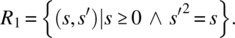
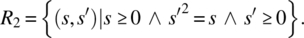
If one asks junior computer science (CS) students in a programming course to write a C++ function that reads a real number and compute its square root, they would rush immediately to their computers to write code and run it; and yet this problem statement, despite being simple and short, leaves many questions unanswered. Consider that this statement may be interpreted in a wide range of manners, leading to a wide range of possible specifications, where space S is defined to be the set of real numbers:
- Only nonnegative arguments will be submitted; the output is a (positive or nonpositive) square root of the input value:
- Only non-negative arguments will be submitted; the output is the nonnegative square root of the input value:
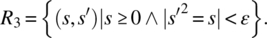
-
Only nonnegative arguments will be submitted; the output is an approximation (within a precision ε) of a (positive or non-positive) square root of the input value:
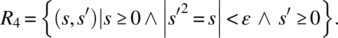
- Only nonnegative arguments will be submitted; the output is an approximation (within a precision ε) of the non-negative square root of the input value:
- Negative arguments may also be submitted; for negative arguments, the output is −1; for nonnegative arguments, the output is a (positive or nonpositive) square root of the input value:

- Negative arguments may also be submitted; for negative arguments, the output is −1; for nonnegative arguments, the output is the nonnegative square root of the input value:

- Negative arguments may also be submitted; for negative arguments, the output is arbitrary; for nonnegative arguments, the output is an approximation (within a precision ε) of a (positive or nonpositive) square root of the input value:

- Negative arguments may also be submitted; for negative arguments, the output is arbitrary; for nonnegative arguments, the output is an approximation (within a precision ε) of the non-negative square root of the input value:

- Only nonnegative arguments will be submitted; the output must be within ε of the exact square root of the input (comparison with specification R4: Precision ε applies to the square root scale rather than the square scale):
We could go on and on. This simple example highlights two lessons: First, the importance of precision in specifying program requirements and second, the premise that relations enable us to achieve the required precision.
As a second illustrative example, consider the following requirement pertaining to space S defined by an array a[1..N] of some type, where N is greater than or equal to 1, a variable x of the same type, and an index variable k, which we use to address array a: Search x in a and place its index in k . Again, this simple requirement lends itself to a wide range of interpretations, some of which we write as follows, along with their relational representation:
- Variable x is known to be in a; place in k an index where x occurs in a.

- Variable x is known to be in a; place in k the first (smallest) index where x occurs in a.

- Variable x is known to be in a; place in k an index where x occurs in a, while preserving a and x.

- Variable x is known to be in a; place in k the first (smallest) index where x occurs in a, while preserving a and x.

- Variable x is not known to be in a; if it is not, place 0 in k; else place in k an index where x occurs in a.

- Variable x is not known to be in a; if it is not, place 0 in k; else place in k the first (smallest) index where x occurs in a.

- Variable x is not known to be in a; if it is not, place 0 in k; else place in k an index where x occurs in a, while preserving a and x.

- Variable x is not known to be in a; if it is not, place 0 in k; else place in k the first (smallest) index where x occurs in a, while preserving a and x.
Note that F1 can be written simply as ![]() since the clause
since the clause ![]() is a logical consequence of
is a logical consequence of ![]() . We draw the reader’s attention to the importance of carefully watching which variables are primed and which are unprimed in a specification. By writing F1 as we did, we mean that the final value of k points to a location in the original array a where the original value of x is located. As written, this relation specifies a search program. If, instead of F1, we had written the specification as follows:
. We draw the reader’s attention to the importance of carefully watching which variables are primed and which are unprimed in a specification. By writing F1 as we did, we mean that the final value of k points to a location in the original array a where the original value of x is located. As written, this relation specifies a search program. If, instead of F1, we had written the specification as follows:
then it would be possible to satisfy this specification by the following simple program:
{k=1; x=a[1];}
If, instead of F1, we had written the specification as follows:
then it would be possible to satisfy this specification by the following simple program:
{k=1; a[1]=x;}
If, instead of F1, we had written the specification as follows:
then it would be possible to satisfy this specification by the following simple program:
{k=1; x=0; a[1]=0;}
Neither of these three programs is performing a search of variable x in array a.
4.3.2 ORDERING SPECIFICATIONS
When we consider specifications on a given space S, we find it natural to order them according to the strength of their requirement, that is, some of them impose more requirements than others. Let us, for the sake of illustration, consider the specifications of the search program written in the previous section:
It is natural/ intuitive to consider that F2 is stronger than F1 since the latter would be satisfied with k′ pointing to any occurrence of x in a, while the former requires that k′ points to the smallest such occurrence. Also, it is natural to consider that F3 is stronger than F1 since the latter requires that a and x be preserved whereas the former does not; for the same reason, F4 is stronger than F2. On the other hand, F5 can be considered stronger than F1 since the latter makes provisions for the case when x is not in a, whereas the former does not; for the same reason, we can consider that F6 is stronger than F2, that F7 is stronger than F3, and that F8 is stronger than F4. These ordering relations are depicted in Figure 4.8.
Figure 4.8 A lattice of refinement.
We notice that F2 and F5 are both considered stronger than F1, but while the former is a subset of F1, the latter is a superset thereof. There appears to be two (nonexclusive) ways for a specification R to be considered stronger than a specification R′: by having a larger domain, and by having fewer images for elements in the common domain. Whence the following definition.
Henceforth, we use the term refines to refer to the property of being a “stronger’” specification. We admit without proof that the relation refines is a partial ordering between specifications, that is, that it is reflexive, antisymmetric, and transitive. We refer to this relation as the refinement ordering. The graph in Figure 4.9 shows two relations, R′ and R″, that refine relation R.

Figure 4.9 R′ and R″ refine R.
4.3.3 SPECIFICATION GENERATION
Let space S be defined by a real array a[1..N] and a real variable x and an index variable k. We are interested to write a relation to reflect the following requirement:
Place in x the largest value of a and in k the smallest index where the largest value occurs.
For example, if array a has the following values,
| 1 | 2 | 3 | 4 | 5 | 6 | 7 | 8 | 9 | 10 | 11 | 12 |
| 8.9 | 9.1 | 5.2 | 9.4 | 9.4 | 0.12 | 4.3 | 8.2 | 9.4 | 3.1 | 2.6 | 9.4 |
then we want x′to be equal to 9.4 and k′ to be equal to 4. Because it is too difficult to specify all the requirements at once, we consider them one by one:
- Place in x a value larger than all the values in the array:

- Place in x an element of the array (note that M1 alone ensures that x′ is greater than all the elements of the array but does not ensure that it is the maximum: 500.0 could be a possible value, for the array aforementioned):

- Place in k′ an index of a where the maximum of the array occurs:
- Ensure that no index smaller than k′ carries the maximum of the array (hence ensuring that k′ is the smallest index):
Then we compute the overall specification as the intersection of M1, M2, M3, and M4, that is,
As a second example, we consider space S made up of three nonnegative real variables x, y, z, and a variable t that represents the enumerated type: {notri, scalene, isosceles, equilateral, right, rightisoceles}. We consider the following requirement:
Given that x, y, and z represent the sides of a triangle, place in t the class of the triangle represented by x, y, and z from the set {notri, scalene, isosceles, equilateral, rightisoceles, right}. We assume that the label “isosceles” is reserved for triangles that are isosceles but not equilateral and that the label ‘right’ is reserved for triangles that are right but not isosceles.
To write this specification, we write one relation for each type of triangle, then form their union. To this effect, we define the following predicates in triplets of real numbers:
Using these predicates, we define the following relations:
Using these relations, we form the relational specification of the triangle classification problem:
From these two examples, we want to discuss the question of how do we generate a complex specification from simple/ elementary specifications?
- In the case of the specification that finds the maximum of the array, we compute the overall specification as the intersection of elementary specifications; in the case of the specification of triangle classification, we compute the overall specification as the union of elementary specifications.
- It appears that we use the intersection when the domains of the elementary specifications are identical and we use the union when the domains of the elementary specifications are disjoint. In the former case we generate the compound specification as the conjunction of elementary properties; whereas in the latter case, we generate the compound specification by case analysis.
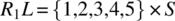
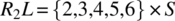
The question that we wish to address then is as follows: Given two relations R1 and R2 on space S, how do we compose them into a specification that captures all the requirements of R1 and all the requirements of R2 (for the sake of completeness) and nothing more (for the sake of minimality), assuming that the domains of R1 and R2 are neither (necessarily) identical nor (necessarily) disjoint? Consider the following graph depicting the configuration of dom(R1) and dom(R2) (Fig. 4.10).
Figure 4.10 Least upper bound of relations R1 and R2.
If we want R to capture all the specification information of R1 and all the specification information of R2, then R has to be identical to R1 outside the domain of R2 and identical to R2 outside the domain of R1, and for each element of the intersection of the domains of R1 and R2, it has to be identical to the intersection of R1 and R2. This justifies the following definition.
This formula is a mere relational representation of the Figure 4.10, depicting how ![]() can be derived from R1 and R2 The following proposition, which we present without proof, gives an important property of the join operator.
can be derived from R1 and R2 The following proposition, which we present without proof, gives an important property of the join operator.
The Figure 4.11 shows an example of two relations R1 and R2 that satisfy the compatibility condition and shows their join.
Figure 4.11 The Join of compatible relations.
To check whether R1 and R2 verify the compatibility condition, we compute the following:
-
 .
. -
 .
.-
 .
.
-
-
 .
.-
 .
.
-
Hence the condition is verified. Since R1 and R2 verify the compatibility condition, their join (![]() ) represents the least refined relation that refines them both. On input 1 (outside the domain of R2), R behaves as R1; on input 6 (outside the domain of R1), R behaves like R2; and on inputs {2,3,4,5} (the intersection of the domains of R1 and R2), R behaves like the intersection of R1 and R2 (which includes {(2,2),(3,3),(4,4),(5,5)}).
) represents the least refined relation that refines them both. On input 1 (outside the domain of R2), R behaves as R1; on input 6 (outside the domain of R1), R behaves like R2; and on inputs {2,3,4,5} (the intersection of the domains of R1 and R2), R behaves like the intersection of R1 and R2 (which includes {(2,2),(3,3),(4,4),(5,5)}).
As a second example, consider the following relations R1 and R2 (Fig. 4.12).
Figure 4.12 Incompatible relations.
In this case, R1 and R2 do not satisfy the compatibility condition since 4 belongs to the domain of each one of them but does not belong to the domain of their intersection. Indeed, it is not possible to find a relation that refines them simultaneously since R1 assigns images 5 and 6 to 4, where R2 assigns images 2 and 3; there is no value that R may assign to 4 to satisfy both R1 and R2.
4.3.4 SPECIFICATION VALIDATION
The software engineering literature is replete with examples of software projects that fail, not because programmers do not know how to write code or how to test it, but rather because analysts and engineers fail to write valid specifications, that is, specifications that capture all the relevant requirements (for the sake of completeness) and nothing but relevant requirements (for the sake of minimality). Consequently, it is important to validate specifications for completeness and minimality and to invest the necessary resources to this effect before proceeding with subsequent phases of the software lifecycle. In this section, we briefly and cursorily discuss the process of specification validation, in the narrow context of the relational specifications that we introduce in this chapter, with the modest goal of giving the reader some sense of what it may mean to validate a specification.
Let us start with a very simple illustrative example: We consider space S defined by natural variables x and y, and we consider the following requirement:
Increase x while preserving the sum of x and y.
We submit the following relations as possible specifications for this requirement:
We invite the reader to ponder the following questions: which of these specifications is complete; and for those that are complete, which are minimal. The following table shows our answers to these questions (if a specification is not complete, it makes no sense to check its minimality):
| Specification | Complete? | Minimal? | Valid? |
|
|
No | N/A | No |
|
|
No | N/A | No |
|
|
Yes | No | No |
|
|
No | N/A | No |
|
|
Yes | Yes | Yes |
|
|
Yes | Yes | Yes |
|
|
Yes | No | No |
|
|
Yes | No | No |
Specifications N5 and N6 are complete and minimal (and are identical, in fact); they specify that x must be increased while preserving the sum of x and y. Specifications N1 and N2 are not complete because they do not stipulate that x must increase (they allow it to stay constant); and specification N4 is not complete because it fails to specify that the sum of x and y must be preserved. Specifications N3, N7, and N8 are complete but not minimal because they specify by how much x must be increased, which is not stipulated in the requirement.
In the example aforementioned, we wrote the specifications on the basis of the proposed requirement (to Increase x while preserving the sum of x and y) and we judged the completeness and minimality of candidate specifications by considering the same source, that is, the proposed requirement. If the same person or group is tasked with generating the candidate specifications and judging their validity (completeness and minimality), then the same biases that cause the person to write invalid specifications may cause him/ her to overlook the invalidity of their specification. The only way to ensure a measure of confidence in the validation of the specification is to separate the team that generates the specification from the team that validates it. To this effect, we propose the following two-team, two-phase approach:
| Activity Phase | Specification Generation | Specification Validation |
| Specification Generation | Generating the specification from sources of requirements | Generating validation data from the same sources of requirements |
| Specification Validation | Updating the specification according to feedback from the validation team | Testing the specification against the validation data generated earlier |
- The Specification Generation Phase: In the specification generation phase, the specification team generates the specification by referring to all the sources of requirements (requirements documents). Using the exact same sources, the validation team generates validation data that it intends to test the specification against. We distinguish between two types of validation data, which are as follows:
- Completeness properties: These are properties that the specification must have but the validation team suspects the specification team may fail to record.
- Minimality properties: These are properties that the specification must not have but the validation team suspects the specification team may record inadvertently. For the sake of redundancy, the specification team and the validation team must work independently of each other.
- The Specification Validation Phase: In the specification validation phase, the validation team tests the specification against completeness and minimality data generated in the previous phase, while the specification team updates the specification if it turns out that it was not complete or not minimal.
It remains to discuss the following: what form does the validation data take, and how does one test a specification against the generated validation data. The answers to these questions are given in the following definitions.
Implicit in this definition is that a good completeness property is one that has the potential to detect an incomplete specification; in other words, a good completeness property is one that the validation team believes the specifier team may have overlooked.
Implicit in this definition is that a good minimality property is one that has the potential to detect a nonminimal specification; in other words, a good minimality property is one that the validation team believes the specifier team may have inadvertently recorded in the specification.
Completeness and minimality are not absolute attributes but rather relative with respect to selected completeness and minimality properties, as provided in the following definition.
We admit without proof that if R refines all of V1, V2, …, Vn, then it refines their join. Hence, the range of valid specifications with respect to completeness properties ![]() and minimality properties
and minimality properties ![]() is represented in the Figure 4.13.
is represented in the Figure 4.13.
Figure 4.13 Range of valid specifications.
As a illustrative example of specification validation, consider the following requirement pertaining to space S defined by an array a[1..N] of some type, a variable x of the same type, and an index variable k, which we use to address array a: Given that x is known to be in a , place in k the smallest index where x occurs. This is a variation of the example discussed in Section 4.2.1.
4.3.4.1 Specification Generation Phase
Examples of completeness properties include the following:
- If each cell of array a contains the index of that cell and if x=1, then k′ should be 1.

-
If array a contains 1 everywhere and x=1, then k′ should be 1.

- If array a contains the sequence 1..N in increasing order and x=N, then k′ should be N.
Examples of minimality properties include the following:
- There is no requirement to preserve x.

- There is no requirement to preserve a.
4.3.4.2 Specification Validation Phase
So far, we have looked at the requirements documentation, but we have not looked at candidate specifications; generating validation data independently of specification generation is important, for the sake of redundancy. Now, let us consider a candidate specification and check whether it is complete with respect to the completeness properties and minimal with respect to the minimality properties. We consider specification F2, introduced in Section 4.2.1 as
To prove that F2 refines V1, we must prove that F2 has a larger domain than V1 and that the restriction of F2 to the domain of V1 is a subset of V1. We find the following:
Clearly, V1L is a subset of F2L. We compute the restriction of F2 to V1L, and we find the following:
![]()
= {substitution}
![]()
= {simplification}
![]()
= {logic simplification}
![]()
= {logic simplification}
![]()
= {substitution}
![]()
We now consider the completeness property V2. To prove that F2 refines V2, we must prove that F2 has a larger domain than V2 and that the restriction of F2 to the domain of V2 is a subset of V2. We find the following:
Clearly, V2L is a subset of F2L. We compute the restriction of F2 to V2L, and we find the following:
![]()
= {substitution}
![]()
= {simplification, redundancy}
![]()
= {logic}
![]()
= {substitution}
![]()
We now consider the completeness property V3. To prove that F2 refines V3, we must prove that F2 has a larger domain than V3 and that the restriction of F2 to the domain of V3 is a subset of V3. We find the following:
Clearly, V3L is a subset of F2L. We compute the restriction of F2 to V3L, and we find the following:
![]()
= {substitution}
![]()
= {simplification}
![]()
= {logic}
![]()
= {simplification, redundancy}
![]()
= {substitution}
![]()
We turn our attention to checking the minimality of F2 with respect to W1 and W2.
Because F2 and W1 have the same domain, the only way to prove that F2 does not refine W1 is to prove that ![]() is not a subset of W1. To this effect, we compute the following:
is not a subset of W1. To this effect, we compute the following:
![]()
= { F2 and W1 have the same domain}
![]()
which is not a subset of W1. Hence F2 is minimal with respect to W1. We can prove, likewise, that it is minimal with respect to W2. Indeed, F2 does not preserve x, nor a.
4.4 RELIABILITY VERSUS SAFETY
The introduction of the refinement ordering introduced in this chapter enables us to revisit a concept we had discussed in Chapter 2, namely, the contrast between reliability and safety. As we remember, the reliability of a system is its ability/likelihood of avoiding failure whereas the safety of a system is its ability/likelihood of avoiding catastrophic failure; because catastrophic failures are failures, one may be tempted to argue that a reliable system is necessarily safe but that is not the case. Indeed, reliability and safety are not logical/Boolean properties but stochastic properties, hence the argument that catastrophic failures are failures does not enable us to infer that reliable systems are necessarily safe. Rather, because the stakes attached to meeting the safety requirements are much higher than those attached to meeting the reliability requirement, the threshold of probability that must be reached for a system to be considered safe is much higher than the threshold of probability that must be reached for a system to be considered reliable.
This idea can be elucidated by means of the refinement ordering: Let R be the specification that represents the reliability requirements of a system, and let F be the specification that represents its safety requirements. For the sake of illustration, we consider a simple example of a system that controls the operation of traffic lights at an intersection.
- Specification R captures the requirements that the traffic light must satisfy in terms of how it schedules the green, orange, and red light of each incoming street, along with the walk and do not walk signs for pedestrians crossing the streets. Such requirements must dictate the sequence of light configurations (which streets have green, which streets have orange, which streets have red, which walkways have a walk signal, which walkways have a flashing walk signal, which walkways have a do not walk signal, etc.), as well as how much each configuration lasts in order to optimize traffic flow, fairness, pedestrian safety, and so on.
- Specification F focuses on two safety critical requirements: First that no orthogonal streets have a green light at the same time; and second no street has a green light for cars and pedestrians at the same time.
The following observations are typical of a reliability–safety relationship:
- The stakes attached to violating a safety requirement are much heavier than the stakes attached to a reliability requirement. Violating a reliability requirement may cause a relatively minor inconvenience, such as a traffic jam or a low throughput of vehicles and pedestrians across the intersection; by contrast, violating a safety requirement may cause an accident that involves injuries or loss of life.
- As a consequence of this difference in stakes, we impose different probability thresholds to the different properties. To consider that a system is reliable, it suffices that it meets the reliability requirements with a probability of 0.99 over a unit of operation time (e.g., an hour): having a traffic jam 1% of the time is acceptable. But to consider that a system is safe, we need a higher probability of meeting the safety requirements: having a fatal accident 1% of the time is not acceptable; a probability threshold of 0.999999 is more palatable.
- The reliability requirements specification (R) refines the safety requirements specification (F). If we consider the sample example of traffic lights and we assume that the requirements specification is valid, then the reliability requirement clearly subsumes the safety requirement since any behavior that abides by the reliability requirement excludes that two orthogonal streets have a green light simultaneously or that a street has a green light while at the same time a walkway that crosses it has a walk signal.
- It is much easier to prove that a candidate program satisfies a safety requirement (F) than it is to prove that it satisfies the reliability requirement (R), for the simple reason that a reliability requirement is typically significantly more complicated. Fortunately, because the safety requirement is simpler, we can verify candidate programs against it with greater thoroughness, hence achieve greater confidence (reflected in higher probability) that a candidate program meets this requirement.
The Figure 4.14 shows specifications R and F, ordered by refinement, and illustrates the relationship between the various possible behaviors of candidate programs, with corresponding probabilities of the behaviors in question: reliable behavior, (possibly unreliable but) fail-safe behavior, and unsafe behavior.

Figure 4.14 Safety vs. reliability.
4.5 STATE-BASED SYSTEMS
Whereas specifications we have studied so far are adequate for specifying programs that take an input (or initial state) and map it onto an output (or final state), they are inadequate to represent programs whose response depends not only on their input but also on their internal state; the subject of this section is to explore ways to specify such systems.
4.5.1 A Relational Model
As we recall from our discussion in Section 4.1, specifications have to have two key attributes, which are formality and abstraction. We can achieve formality by using a mathematical notation, which associates precise semantics to each statement. As for abstraction, we can achieve it by ensuring that the specifications describe the externally observable attributes of candidate software products, but do not specify, dictate, or otherwise favor any specific design or implementation.
We consider the following description of a stack data type: A stack is a data type that is used to store items (through operation push()) and to remove them in reverse order (through operation pop()); operation top() returns the most recently stored item that has not been removed, operation size() returns the number of items stored and not removed, and operation empty() tells whether the stack has any items stored; operation init() reinitializes the stack to an initial situation, where it contains no elements. Imagine that we want to specify a stack without saying anything about how to implement it. How would we do it? Most data structure courses introduce stacks by showing a data structure made up of an array and an index into the array and by explaining how push and pop operations affect the array and its index; but such an approach violates the principle of abstraction since it specifies the stack by describing a possible implementation thereof. An alternative could be to specify the stack by means of an abstract list, along with list operations, without specifying how the list is implemented. We argue that this too violates the principle of abstraction as it dictates a preferred implementation; in fact, a stack does not necessarily require a list of elements, regardless of how the list is represented, as we show here.
- Consider that a stack that stores identical elements can be implemented by a simple natural number, say n:
-
init(): {n=0;} -
push(a): {n=n+1;} // a is the only value that can be //stacked -
pop(): {if (n>0) {n=n-1;}} -
top(): {if (n>0) {return a;} else {return error;}} -
size(): {return n;} -
empty(): {return (n==0);}
-
- Consider that a stack that stores two possible symbols (e.g., ‘{’ and ‘}’) can also be implemented without any form of list, using a simple natural number, say n:
-
init(): {n=1;} -
push(a): {n=2*n+code(a);} // where code(a) maps the two //symbols onto 0 nd 1. -
pop(): {if (n>1) {n=n div 2;}} -
top(): {if (n==1) {return error;} else {return decode(n mod 2);}} // ecode() is the inverse of code(). -
size(): {return floor(log2(n));} -
empty(): {return (n==1);}
-
- We can likewise implement a stack that stores any number (k) of symbols by using base-k numeration rather than base 2 (used earlier).
Hence, for the sake of abstraction, we resolve to specify the stack by describing its externally observable behavior, without making any assumption, regardless of how vague, about its internal structure. To this effect, we specify a stack by means of three parameters, which are as follows:
- An input space, say X, which includes all the operations that may be invoked on the stack. Hence,
 , where itemtype is the data type of the items we envision to store in the stack. We distinguish, in set X, between inputs that affect the state of the stack (namely,
  ) and inputs that merely report on it (namely,
  ).
).From the set of inputs X, we build the set of input histories, H, where an input history is a sequence of inputs; this is needed because the behavior of the stack is not determined solely by the current input but involves past inputs as well.
- Hence, we introduce the set of input histories,
 .
.
- Hence, we introduce the set of input histories,
- An output space, say Y, which includes all the values returned by all the elements of VX. In the case of the stack, the output space is as follows:
 , which correspond, respectively, to inputs top, size, and empty.
 - A relation from H to Y, which represents the pairs of the form (h, y), where h is an input history and y is an output that the specifier considers correct for h. We denote this relation by stack and we use the notation stack (h) to refer to the image of h by stack (if that image is unique) or to the set of images of h by stack (if h has more than one image). We present here some pairs of the form (h, y) for relation stack:
-
 .
. -
 .
. -
 .
. -
 .
. -
 .
.
-
We can go on describing possible input histories and corresponding outputs. In doing so, we are specifying how operations interact with each other but we are not prescribing how each operation behaves; this leaves maximum latitude to the designer, as mandated by the principle of abstraction.
It is clearly impractical to specify data types by listing elements of their relations; in the next section, we explore a closed-form representation for such relations.
4.5.2 AXIOMATIC REPRESENTATION
We propose to represent the relation of a specification by means of an inductive notation, where we do induction on the structure of the input history; this notation includes two parts, which are as follows:
- Axioms, which represent the behavior of the system for trivial input histories.
- Rules, which represent the behavior of the system for complex input histories as a function of its behavior for simpler input histories.
4.5.2.1 Specification of a Stack
As an illustration, we represent the specification of the stack using axioms and rules. Throughout this presentation, we let a be an arbitrary element of itemtype and y an arbitrary element of Y; also, we let h, h′, h″ be arbitrary elements of H and h+ an arbitrary non-null element of H.
Axioms. We use axioms to represent the output of input histories that end with an operation in set VX (that reports on the state), namely in this case top, size, and empty. It is understood that input histories that end with an operation in set AX (that affects the state) produce no meaningful output; hence we assume that for such input histories, the output is any element of Y.
- Top Axioms
- stack(init.top) = error.
Seeking the top of an empty stack returns an error.
- stack(init.h.push(a).top) = a.
Operation top returns the most recently stacked item.
- stack(init.top) = error.
- Size Axiom
- stack(init.size) = 0.
The size of an empty stack is zero.
- stack(init.size) = 0.
- Empty Axioms
- stack(init.empty) = true.
An initial stack is empty.
- stack(init.push(a).empty) = false.
A stack that contains element a is not empty.
- stack(init.empty) = true.
Rules: Whereas axioms characterize the behavior of the stack for simple input sequences, rules establish relations between the behavior of the stack for complex input histories and their behavior for simpler input histories.
- Init Rule
- stack(h’.init.h) = stack(init.h).
Operation init reinitializes the stack; whether sequence h′ intervened prior to init or did not makes no difference for the future behavior (h) of the stack.
- stack(h’.init.h) = stack(init.h).
- Init Pop Rule
- stack(init.pop.h) = stack(init.h).
A pop operation on an empty stack has no effect: whether it occurred or did not occur makes no difference for the future behavior (h) of the stack.
- stack(init.pop.h) = stack(init.h).
- Push Pop Rule
- stack(init.h.push(a).pop.h+) = stack(init.h.h+).
A pop operation cancels the most recent push: whether the sequence push(a).pop occurred or did not makes no difference to the future behavior of the stack, though not to the present (if h ends with an operation in VX, we could not say that stack(init.h)=stack(init.h.push(a).pop) as the left-hand side returns a specific value but the right-hand side returns an arbitrary value).
- stack(init.h.push(a).pop.h+) = stack(init.h.h+).
- Size Rule
- stack(init.h.push(a).size) = 1+stack(init.h.size).
We assume that the stack is unbounded; hence any push operation increases the size by 1.
- stack(init.h.push(a).size) = 1+stack(init.h.size).
- Empty Rules
- stack(init.h.push(a).h’.empty) ⇒ stack(init.h.h’.empty).
- stack(init.h.h’.empty) ⇒ stack(init.h.pop.h’.empty).
Removing a push or adding a pop to the input history of a stack makes it more empty (i.e., if it was empty prior to removing push or adding pop, it is a fortiori empty afterward).
- VX Rules
- stack(init.h.top.h+) = stack(init.h.h+).
- (init.h.size.h+) = stack(init.h.h+).
- (init.h.empty.h+) = stack(init.h.h+).
VX operations leave no trace of their passage; once they are serviced and another operation follows them, they are forgotten: whether they occurred or did not occur has no impact on the future behavior of the stack.
We have written a closed-form specification of the stack in such a way that we describe solely the externally observable properties of the stack, without any reference to how a stack ought to be implemented; a programmer who reviews this specification has all the latitude he/she needs to implement this stack as he/she sees fit.
4.5.2.2 Specification of a Queue
We discuss how to represent the specification of a queue, in the same way that we wrote the specification of a stack earlier. We represent in turn the input space (from which we infer the set of input histories), then the output space, then the relation, which we denote by queue.
Input Space. We let X be defined as X = {init, dequeue, front, size, empty} ∪ {enqueue} × itemtype. We partition this set into AX = {init, enqueue, dequeue} and VX = {front, size, empty}. We let H be the set of sequences of elements of X.
Output Space. We let the output space be defined as Y = itemtype ∪ integer ∪ Boolean ∪ {error}.
Axioms. We propose the following axioms:
- Front Axioms
- queue(init.front) = error.Invoking front on an empty queue returns an error.
- queue(init.enqueue(a).enqueue*().front) = a,where enqueue(_)* designates an arbitrary number (including zero) of enqueue operations, involving arbitrary items as parameters. Interpretation: Invoking front on a non-empty queue returns the first element enqueued.
- Size Axioms
- queue(init.size) = 0.The size of an empty queue is zero.
- Empty Axioms
- queue(init.empty) = true.
- queue(init.enqueue(a).empty) = false.An initial queue is empty. A queue in which an element has been enqueued is not empty.
Rules: We propose the following rules.
- Init Rule
- queue(h’.init.h) = queue(init.h).The init operation reinitializes the stack, that is, renders all past input history immaterial.
- Init Dequeue Rule
- queue(init.dequeue.h) = queue(init.h)A dequeue operation executed on an empty queue has no effect.
- Enqueue Dequeue Rule
- queue(init.enqueue(a).enqueue*(_).dequeue.h) = queue(init.enqueue*(_).h)A dequeue operation cancels the first enqueue, by virtue of the first in, first out (FIFO) policy of queues.
- Size Rule
- queue(init.h.enqueue(a).size) = 1+queue(init.h.size).Assuming queues of unbounded size, any enqueue operation increases the size of the queue by 1.
- Empty Rules
- queue(init.h.enqueue(a).h’.empty) ⇒ queue(init.h.h’.empty).
- stack(init.h.h’.empty) ⇒ stack(init.h.dequeue.h’.empty).Removing an enqueue or adding a dequeue to the input history of a queue makes it more empty (i.e., if it was empty prior to removing enqueue or adding dequeue, it is a fortiori empty afterward).
- VX Rules
- queue(init.h.front.h+) = queue(init.h.h+).
- queue(init.h.size.h+) = queue(init.h.h+).
- queue(init.h.empty.h+) = queue(init.h.h+).VX operations leave no trace of their passage; once they are serviced and another operation follows them, they are forgotten: whether they occurred or did not occur has no impact on the future behavior of the queue.
4.5.2.3 Specification of a Set
As a third illustrative example, we discuss how to represent the specification of a set, in the same way that we wrote the specifications of a stack and a queue earlier. We represent in turn the input space (from which we infer the set of input histories), then the output space, then the relation, which we denote by set.
Input Space: Before we introduce the input space, let us review quickly what we want this set abstract data type (ADT) to do: we want the ability to reinitialize the set, pick a random element of the set, enumerate all its elements, and return its smallest element and its largest element (assuming its elements are ordered). Also, we want to be able to insert, delete, and search designated elements of the set. Hence, we let X be defined as
X = {init, pick, min, max, enumerate, size} ∪ {insert, delete, search}× itemtype.
We partition this set into AX = {init, insert, delete} and VX = {pick, min, max, size, enumerate, search}. We let H be the set of sequences of elements of X.
Output Space: We let the output space be defined as
Y = itemtype ∪ P(itemtype) ∪ {error} ∪ integer ∪ boolean,
where P(itemtype) is the power set of itemtype.
Axioms: We propose the following axioms:
- Pick Axioms
- set(init.pick) = error.One cannot pick an element from an empty set.
- Set(init.h.insert(a).pick) = a.If a is an element of the set, then it is a possible pick; we will add a commutativity rule later to make it possible to pick other elements than the most recently inserted element.
- Size Axiom
- set(init.size) = 0.The size of an empty set is zero.
- Enumerate Axiom
- set(init.enumerate) = ∅.The enumeration of an empty set returns empty.
- Search Axiom
- set(init.search(a)) = false.The search of a in an empty set returns false.
- Min Axiom
- set(init.min) = +∞.Plus infinity is the neutral element of operation min.
-
Max Axiom
- set(init.max) = −∞.Minus infinity is the neutral element of operation max.
Rules: We propose the followng rules:
- Init Rule
- set(h’.init.h) = set(init.h).Operation init makes the previous history irrelevant.
- Null Delete Rule
- set(init.delete(a).h) = set(init.h).A delete operation has no effect on an empty set.
- Insert Delete Rule
- set(init.insert(a).delete(a).h) = set(init.h).Operation delete cancels the effect of operation insert.
- Idempotence Rule
- Insert Insert Ruleset(init.h’.insert(a).insert(a).h) = set(init.h’.insert(a).h) if is already in the set, inserting it makes no difference.
- Commutativity Rule
- set(init.h’.op1(a).op2(b).h) = set(init.h’.op2(b).op1(a).h).where op1 and op2 are any of insert and delete and a and b are distinct. Interpretation: The order of operations of insert and delete of distinct elements is immaterial.
- Size Rules
- If set(init.h.search(a)) = true then set(init.h.insert(a).size) = set(init.h.size).
- If set(init.h.search(a)) = false then set(init.h.insert(a).size) = 1+set(init.h.size).Operation insert(a) increases the size of the set only if element a is not in the set prior to insertion.
- Inductive Rules
- set(init.h.insert(a).search(b)) = (a=b) ∨ set(init.h.search(b)).If (a=b) then return true (since b is found in the set), else check prior to the insertion of a.
- set(init.h.insert(a).enumerate) = {a} ∪ set(init.h.enumerate).If a has been inserted, it should be enumerated.
- set(init.h.insert(a).min) = MIN (a, set(init.h.min)).Inductive argument on the min.
- set(init.h.insert(a).max) = MAX (a, set(init.h.max)).Inductive argument on the max.
- VX Rules
- set(init.h.search(a).h+) = set(init.h.h+).
- set(init.h.pick.h+) = set(init.h.h+).
- set(init.h.enumerate.h+) = set(init.h.h+).
- set(init.h.size.h+) = set(init.h.h+).
- set(init.h.min.h+) = set(init.h.h+).
- set(init.h.max.h+) = set(init.h.h+).VX operations leave no trace of their passage once they have been passed.
4.5.3 SPECIFICATION VALIDATION
In the previous section, we have written specifications of a number of ADTs, namely, a stack, a queue, and a set. How do we know that our specifications are valid, that is, that they capture all the properties we want them to capture (completeness) and nothing else (minimality)? To bring a measure of confidence in the validity of these specifications, we envision a validation process, similar to the process we advocated in Section 4.2.3, though this time (for the sake of simplicity) we focus solely on completeness. We imagine that while we are writing these specifications, an independent verification and validation team is generating formulas of the form
for different values of h and y, on the grounds that whatever we write in our specification should logically imply these statements. Then the validation step consists in checking that the proposed formulas can be inferred from the axioms and rules of our specification. If they do, then we can conclude that our specification is complete with respect to the proposed formulas; if not, then we need to check with the verification and validation team to see whether our specification is incomplete or perhaps the validation data is erroneous.
For the sake of illustration, we check whether our specification is valid with respect to the formulas written in Section 4.3 as sample input/output pairs of our stack specification:
For V1, we find the following:
stack(pop.init.push(a).init.push(a).top)
= {by the init Rule}
stack(init.push(a).top)
= {by the second top axiom}
a. QED
For V2, we find the following:
stack(pop.init.pop.push(a).push(b).top.top)
= {by the init Rule}
stack(init.pop.push(a).push(b).top.top)
= {by the VX Rule pertaining to top}
stack(init.pop.push(a).push(b).top)
= {by the second top axiom}
b. QED
For V3, we find the following:
stack(init.pop.push(a).pop.push(a).pop.push(a).size)
= {by the init pop Rule}
stack(init.push(a).pop.push(a).pop.push(a).size)
= {by the push pop Rule, applied twice}
stack(init.push(a).size)
= {by the size Rule}
1+stack(init.size)
= {by the size axiom}
1. QED
For V4, we find the following:
stack(pop.push(a).pop.init.pop.push(a).top.push(a).top.push(a).pop.empty)
= {by the init rule}
stack(init.pop.push(a).top.push(a).top.push(a).pop.empty)
= {by the init pop rule}
stack(init.push(a).top.push(a).top.push(a).pop.empty)
= {by the VX rule, as it pertains to top}
stack(init.push(a).push(a).push(a).pop.empty)
= {by the push pop rule}
stack(init.push(a).push(a).empty)
⇒ {by the empty rule}
stack(init.push(a).empty)
= {by the empty axiom}
false.
If the left-hand side logically implies false, then it is false. QED
For V5, we find the following:
stack(init.pop.pop.pop.push(a).push(b).push(c).top.push(c).push(b).empty.top)
= {by virtue of the VX rules, applied to empty}
stack(init.pop.pop.pop.push(a).push(b).push(c).top.push(c).push(b).top)
= {by virtue of the second top axiom}
b. QED
Because our specification has survived five tests unscathed, we gain a bit more confidence in its validity.
4.6 CHAPTER SUMMARY
The main ideas/concepts that you need to keep from this chapter are the following:
- The algebra of relations, including operations, and properties.
- Principles of sound specification, and how relations support these.
- The concept of join of relations, its significance, and its role in specification generation.
- The concept of refinement, its significance, and its role in specification validation.
- The relational specification of systems that maintain an internal state.
- The axiomatic representation of the relational specification of systems that maintain a state.
- The generation and validation of axiomatic specifications.
4.7 EXERCISES
- 4.1. Given relations R and Q on set S, write a relational expression that represents the following: the prerestriction of R to the domain of Q; the prerestriction of R to the range of Q; the postrestriction of R to the domain of Q; the postrestriction of R to the range of Q.
- 4.2. Consider the following relations on the set S of natural numbers:
- R = {(s,s′)| s′= 7s}
- R′ = {(s,s′)| s′ = s+5}
Compute the following:
- dom(R), rng(R).
- dom(R′), rng(R′).
- R•R′. dom(R.R′).
- R′•R. dom(R′.R).
- Prerestriction of R to A = {s| s mod 5=0}.
- Postrestriction of R′to B = {s| s<4}.
- 4.3. Consider the following relations on the set S of natural numbers (starting at zero).
- R ={(s,s′)| s′ = s-7}
- R′={(s,s′)| s′ = 5s – 32}
Compute the following expressions:
- dom(R), rng(R).
- dom(R′), rng(R′).
-
 , and
, and 
-
 , and
, and  .
. - R · R′, and dom (R · R′).
- R′ · R, and dom (R′ · R).
- 4.4. For each relation R given here on space S defined by natural variables x and y, tell whether R has the properties defined in Section 4.2.3.
- R = {(s,s′)| x+y = x′+y′}
- R = {(s,s′)| x′ = x+1 ∧ y′ = y−1}
- R = {(s,s′)| x ≥ x′ ∧ y’ = y}
- R = {(s,s′)| x−y ≥ x′− y′}
- R = {(s,s′)| x ≥ 1 ∧ y ≥ x}
- 4.5. Let S be the set of persons and let P and M be the following relations on S:
- P = {(s,s’)| s’ is a parent of s}.
- M = {(s,s’)| s is male}.
From these three relations, compose the following relations: female (the complement of male), mother, father, daughter, son, half-sibling, sibling, half brother, half sister, brother, sister, maternal grandfather, paternal grandfather, maternal grandmother, paternal grandmother, grandson, granddaughter, uncle, aunt, niece, nephew, and cousin. All of these relations can be built from P and M.
- 4.6. Consider the square root specification given in Section 4.3.1; give five more possible interpretations of the square root requirement, and present a relation for each.
- 4.7. Consider the specification of the search programs, given in Section 4.3.2. Write five new interpretations, along with corresponding relations. Hint: Consider, for example, the situation where a and x are preserved whether x is or is not in a; or the case where no output requirement is imposed when x is not in a.
- 4.8. Consider the following specifications on space S defined by an array a[1..N] of real numbers and a variable x of type real and say whether or not they represent the specification of a program to compute the sum of a into x; if not, give an example of a program that satisfies the specification but is not computing the sum of a into x.
-
- 4.9 Consider the square root specifications R1 … R9 given in Section 4.3.1. Rank them by the refinement ordering and draw a graph showing their refinement relations, similar to that given for the search specifications F1 … F8.
- 4.10 Consider a space S defined by an array a[1..N] of type T, an index variable k and a variable x of type T. Write the following specifications and rank them by strength:
- Place in x the largest element of a.
- Place in x the largest element of a and in k an index where the largest element of a occurs.
- Place in x the largest element of a and in k the largest index where the largest element of a occurs.
- Place in x the largest element of a and in k an index where the largest element of a occurs, while preserving a.
- 4.11 Consider a space S defined by an array a[1..N] of type T, an index variable k and a variable x of type T. Write the following specifications and rank them by strength:
- Place in x a value less than or equal to all the elements of the array.
- Place in x an arbitrary value of the array.
- Place in x an arbitrary value of the array and in k an index where x occurs.
- Place in x the smallest element of the array and in k an index where x occurs.
- Place in x the smallest element of the array and in k the smallest index where x occurs.
- 4.12 Prove that the refines relation between relational specifications is a partial ordering relation; that it is reflexive, antisymmetric and transitive.
- 4.13 Let space S be defined by three variables a, b, c of type natural, and consider the requirement that these three variables be rearranged in increasing order, that is, we want to permute their values in such a way that a′≤b′≤c′. Write the relational specification of this requirement, by proceeding: first by case analysis (consider all the possible orderings of the three values of a, b, c) and second, by conjunction of properties (consider all the relations that must hold between a, b, c and a′, b′, c′).
- 4.14 Consider the following specifications on space S defined by an array a[1..N] of some type, a variable x of the same type, and an index variable k, which we use to address array a.
Do these specifications satisfy the compatibility condition? If so, compute their join. If not, explain why.
-
- 4.15. Consider the following specifications on space S defined by an array a[1..N] of some type, a variable x of the same type, and an index variable k, which we use to address array a.
Do specifications F5 and F9 satisfy the compatibility condition? If so, compute their join. If not, explain why.
-
- 4.16. Consider the following specifications on space S defined by an array a[1..N] of some type, a variable x of the same type, and an index variable k, which we use to address array a.
Do specifications F5 and F10 satisfy the compatibility condition? If so, compute their join. If not, explain why.
-
- 4.17. Check whether Specification F1 (given in Section 4.3.2) is complete with respect to completeness properties V1, V2, V3 and whether it is minimal with respect to minimality properties W1, W2.
- 4.18. Check whether Specification F3 (given in Section 4.3.2) is complete with respect to completeness properties V1, V2, V3 and whether it is minimal with respect to minimality properties W1, W2.
- 4.19. Check whether Specification F4 (given in Section 4.3.2) is complete with respect to completeness properties V1, V2, V3 and whether it is minimal with respect to minimality properties W1, W2.
- 4.20. Check whether Specification F5 (given in Section 4.3.2) is complete with respect to completeness properties V1, V2, V3 and whether it is minimal with respect to minimality properties W1, W2.
- 4.21. Check whether Specification F6 (given in Section 4.3.2) is complete with respect to completeness properties V1, V2, V3 and whether it is minimal with respect to minimality properties W1, W2.
- 4.22. Check whether Specification F7 (given in Section 4.3.2) is complete with respect to completeness properties V1, V2, V3 and whether it is minimal with respect to minimality properties W1, W2.
- 4.23. Check whether Specification F8 (given in Section 4.3.2) is complete with respect to completeness properties V1, V2, V3 and whether it is minimal with respect to minimality properties W1, W2.
- 4.24. Generate validation data for the stack specification given in Section 4.5.2.1, and chek its validity against your data.
- 4.25. Generate validation data for the queue specification given in Section 4.5.2.2, and check its validity against your data.
- 4.26. Generate validation data for the set specification given in Section 4.5.2.3, and check its validity against your data.
- 4.27. Follow the example discussed in Section 4.5.1 to derive a stack that stores four symbols, e.g. the arithmetic operators +, −, *, and /.
4.8 PROBLEMS
4.1. This ADT stores and retrieves elements in a linearly ordered structure. We let the list be defined by the following operations:
AX-operations: These are operations that alter the state of the ADT but produce no visible output.
- init: This operation initializes or re-initializes the list to empty.
- insertlast (itemtype x): This operation inserts x at the end of the list.
- insertfirst (itemtype x): This operation inserts x at the beginning of the list.
- insertat (itemtype x, integer n): If the size of the list allows, this operation inserts x at position n; else it does not change the list.
- deletelast (): This operation deletes the element at the end of the list.
- deletefirst (): This operation deletes the element at the beginning of the list.
- deletetat (integer n): If the size of the list allows, this operation deletes the element at position n; else it does not change the list.
VX-operations: These are operations that return values but do not change the state.
- boolean: empty (): It returns T if and only if the list is empty.
- integer: size (): It returns the number of elements in the list.
- boolean: search (itemtype x): It tells whether x is in the list.
- integer: multisearch (itemtype x): It gives the multiplicity of x in the list.
- itemtype: choose (): It returns an arbitrary element of the list.
- itemtype: first (): It returns the first element in the list.
- itemtype: last (): It returns the last element in the list.
- itemtype: smallest (): It returns the smallest element.
- itemtype: largest (): It returns the largest element.
Write this specification and validate it. If this work is done in a team, divide the team in two, for specification and specification validation. Hint: Convert all insert operations into insertlast operations, and all delete operations into deletelast operations; then specify insertlast and deletelast.
4.2. In discrete mathematics, a multiset is a collection of objects where duplication is permitted. We let multiset be defined by the following operations:
- AX-operations: These are operations that alter the state of the ADT but produce no visible output.
- init: This operation initializes or re-initializes the multiset to empty.
- insert (itemtype x): If x is not in the multiset, this operation adds it; if not, it increments its multiplicity.
- insert (itemtype x, integer n): Inserts n copies of x, where n is non-negative.
- remove (itemtype x): If x is not in the set, then this operation is null; if x does belong in a single copy, it no longer exists in the set; if x belongs in multiple copies, its multiplicity is reduced by 1.
- remove (itemtype x, integer n): It performs remove(x) n times.
- removeall (itemtype x): If x does not belong to the multiset, then this operation is null; else all instances of x are removed.
- removeany(): It removes an arbitrary element of the set, reducing its multiplicity by 1; if the set is empty, this operation is null.
- eraseany(): It removes all the instances of an arbitrary element; if the multiset is empty, this operation is null.
-
VX-operations: These are operations that return values but do not change the state.
- boolean: empty (): It returns T if and only if the set is empty.
- integer: size (): It returns the number of distinct elements.
- integer: multisize (): It returns the multisize of the multiset.
- boolean: search (itemtype x): It tells whether x is in the multiset.
- integer: multisearch (itemtype x): It gives the multiplicity of x.
- itemtype: choose (): It returns an arbitrary element of the multiset.
- itemtype* list (): It lists the elements of the multiset.
- itemtype* list (integer n): It lists the elements of the multiset with a multiplicity greater than or equal to n.
- itemtype: least (): It returns an element with minimal multiplicity.
- itemtype: most (): It returns an element with maximal multiplicity.
- itemtype: smallest (): It returns the smallest element.
- itemtype: largest (): It returns the largest element.
Write this specification and validate it. If this work is done in a team, divide the team in two, for specification and specification validation.
4.9 BIBLIOGRAPHIC NOTES
Software specification has been the subject of active research since the early days of software engineering, highlighting both the criticality and the difficulty of this phase and its products; it is impossible to do justice to all the work that was published in this area or to any significant portion thereof. We will merely cite a few of the specification languages that have emerged: Z, a relational notation that has been widely used in industry and academia (Spivey, 1998); B, a relational notation that has an object-oriented flavor, and supports refinement, in addition to specification (Abrial, 1996); Alloy, a language inspired by Z and B and used to represent structures by means of sets of constraints (Jackson, 2011). For a general overview of specification languages and issues, consult (Habrias and Frappier, 2013).