
Chapter 6
Further modeling issues
Chapters 1 to 3 introduced the basic MSPC approach that is applied to the chemical reaction and the distillation processes in Chapters 4 and 5, respectively. This chapter extends the coverage of MSPC modeling methods by discussing the following and practically important aspects:
Section 6.1 introduces a maximum likelihood formulation for simultaneously estimating an unknown diagonal error covariance matrix and the model subspace, and covers cases where ![]() is known but not of the form
is known but not of the form ![]() .
.
Section 6.2 discusses the accuracy of estimating PLS models and compares them with OLS models with respect to the relevant case that the input variables are highly correlated. The section then extends the data structure in 2.23, 2.24 and 2.51 by including an error term for the input variable set, which yields an error-in-variable (Söderström 2007) or total least squares (van Huffel and Vandewalle 1991) data structure. The section finally introduces a maximum likelihood formulation for PLS and MRPLS models to identify error-in-variable estimates of the LV sets.
Outliers, which are, at first glance, samples associated with a very large error or are simply different from the majority of samples, can profoundly affect the accuracy of statistical estimates (Rousseeuw and Hubert 2011). Section 6.3 summarizes methods for a robust estimation of PCA and PLS models by reducing the impact of outliers upon the estimation procedure and trimming approaches that exclude outliers.
Section 6.4 describes how a small reference set, that is, a set that only contains few reference samples, can adversely affect the accuracy of the estimation of MSPC models. The section stresses the importance of statistical independence for determining the Hotelling's T2 statistics and also discusses a cross-validatory approach for the residual-based Q statistics.
Finally, Section 6.5 provides a tutorial session including short questions and small projects to help familiarization with the material of this chapter. This enhances the learning outcomes, which describes important and practically relevant extensions of the conventional MSPC methodology, summarized in Chapters 1 to 3.
6.1 Accuracy of estimating PCA models
This section discusses how to consistently estimate PCA models if ![]() , which includes the estimation of the model subspace and
, which includes the estimation of the model subspace and ![]() . The section first revises the underlying assumptions for consistently estimating a PCA model by applying the eigendecomposition of
. The section first revises the underlying assumptions for consistently estimating a PCA model by applying the eigendecomposition of ![]() in Subsection 6.1.1. Next, Subsection 6.1.2 presents two illustrative examples to demonstrate that a general structure of the error covariance matrix, that is,
in Subsection 6.1.1. Next, Subsection 6.1.2 presents two illustrative examples to demonstrate that a general structure of the error covariance matrix, that is, ![]() yields an inconsistent estimation of the model subspace.
yields an inconsistent estimation of the model subspace.
Under the assumption that the error covariance matrix is known a priori, Subsection 6.1.3 develops a maximum likelihood formulation to consistently estimate the orientation of the model and residual subspaces. If ![]() is unknown, Subsection 6.1.4 introduces an approach for a simultaneous estimation of the model subspace and
is unknown, Subsection 6.1.4 introduces an approach for a simultaneous estimation of the model subspace and ![]() using a Cholesky decomposition. Subsection 6.1.5 then presents a simulation example to show a simultaneous estimation of the model subspace and
using a Cholesky decomposition. Subsection 6.1.5 then presents a simulation example to show a simultaneous estimation of the model subspace and ![]() for a known number of source signals n. Assuming n is unknown, Subsection 6.1.6 then develops a stopping rule to estimate the number of source signals.
for a known number of source signals n. Assuming n is unknown, Subsection 6.1.6 then develops a stopping rule to estimate the number of source signals.
Subsection 6.1.7 revisits the maximum likelihood estimates of the model and residual subspaces and introduces a re-adjustment to ensure that the loading vectors, spanning both subspaces, point in the direction of maximum variance for the sample projections. Finally, Subsection 6.1.8 puts the material presented in this section together and revisits the application study of the chemical reaction process in Chapter 4. The revised analysis shows that the recorded variable set contains a larger number of source signals than the four signals previously suggested in Chapter 4.
6.1.1 Revisiting the eigendecomposition of 
Equation (2.2) and Table 2.1 show that the data structure for recorded data is
Removing the mean from the recorded variable, the stochastic component is assumed to follow a zero mean multivariate Gaussian distribution with the covariance matrix
6.2 ![]()
Asymptotically, assuming that ![]() the eigendecomposition of
the eigendecomposition of ![]()
6.3 
yields
Given that ![]() and
and ![]() the eigendecomposition of
the eigendecomposition of ![]() provides an asymptotic estimate of
provides an asymptotic estimate of ![]() and allows extracting
and allows extracting ![]()
6.5 
Since the matrix ![]() has orthonormal columns, which follows from Theorem 9.3.3, the term
has orthonormal columns, which follows from Theorem 9.3.3, the term ![]() reduces to
reduces to ![]() and hence
and hence
6.6 
Under the above assumptions, the eigendecomposition of ![]() can be separated into
can be separated into ![]() and
and ![]() , where
, where
6.7 
and
Following the geometric analysis is Section 2.1, 2.2 to 2.5 and Figure 2.2, the model subspace, originally spanned by the column vectors of Ξ, can be spanned by the n retained loading vectors p1, p2, ··· , pn, since
Determining the eigendecomposition of Sss and substituting ![]() into (6.9) gives rise to
into (6.9) gives rise to
6.10 ![]()
Next, re-scaling the eigenvalues of Sss such that ![]() yields
yields
Hence, ![]() , where
, where ![]() is a diagonal scaling matrix. The above relationship therefore shows that
is a diagonal scaling matrix. The above relationship therefore shows that ![]() and hence,
and hence, ![]() .
.
Now, multiplying this identity by ![]() from the left gives rise to
from the left gives rise to
6.12 ![]()
which follows from the fact that the PCA loading vectors are mutually orthonormal. That the discarded eigenvectors, spanning the residual subspace, are orthogonal to the column vectors of Ξ implies that the n eigenvectors stored as column vectors in P span the same model subspace. Consequently, the orientation of the model subspace can be estimated consistently by determining the dominant eigenvectors of ![]()
6.13 ![]()
In other words, the dominant n loading vectors present an orthonormal base that spans the model subspace under the PCA objective function of maximizing the variance of the score variables ![]() . It can therefore be concluded that the loading vectors present an asymptotic approximation of the model subspace, spanned by the column vectors in Ξ. However, this asymptotic property holds true only under the assumption that
. It can therefore be concluded that the loading vectors present an asymptotic approximation of the model subspace, spanned by the column vectors in Ξ. However, this asymptotic property holds true only under the assumption that ![]() is a diagonal matrix with identical entries, which is shown next.
is a diagonal matrix with identical entries, which is shown next.
6.1.2 Two illustrative examples
The first example is based on the simulated process in Section 2.1, where three process variables are determined from two source signals that follow a multivariate Gaussian distribution, ![]() . Equations 2.9 to 2.11 show the exact formulation of this simulation example. The error covariance matrix of 2.11 is therefore of the type
. Equations 2.9 to 2.11 show the exact formulation of this simulation example. The error covariance matrix of 2.11 is therefore of the type ![]() so that the eigendecomposition of
so that the eigendecomposition of ![]() allows a consistent estimation of the model subspace, spanned by the two column vectors of Ξ,
allows a consistent estimation of the model subspace, spanned by the two column vectors of Ξ, ![]() and
and ![]() .
.
Constructing an error covariance matrix that is of a diagonal type but contains different diagonal elements, however, does not yield a consistent estimate of the model subspace according to the discussion in previous subsection. Let ![]() be
be
which produces the following covariance matrix of z0
6.15 
The eigendecomposition of this covariance matrix is
6.16 
To examine the accuracy of estimating the model subspace, the direction of the residual subspace, which is ![]() according to (2.20), can be compared with the third column vector in P
according to (2.20), can be compared with the third column vector in P
As a result, the determined residual subspace departs by a minimum angle of 3.4249° from the correct one. Defining ![]() as a parameter the above analysis demonstrates that this parameter is not equal to 1. Hence, n can only be estimated with a bias (Ljung 1999). Asymptotically,
as a parameter the above analysis demonstrates that this parameter is not equal to 1. Hence, n can only be estimated with a bias (Ljung 1999). Asymptotically, ![]() if
if ![]() and else < 1.
and else < 1.
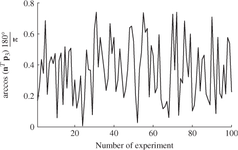
A second example considers a Monte Carlo experiment where the variances for each of the three error variables are determined randomly within the range of ![]() . For a total of 100 experiments, Figure 6.1 shows the uniformly distributed values for each error variance. Applying the same calculation for determining the minimum angle between p3 and n for each set of error variances yields the results shown in Figure 6.2. Angles close to zero, for example in experiments 23 and 51, relate to a set of error variances that are close to each other. On the other hand, larger angles, for example experiments 31, 53, 70, 72 and 90 are produced by significant differences between the error variances.
. For a total of 100 experiments, Figure 6.1 shows the uniformly distributed values for each error variance. Applying the same calculation for determining the minimum angle between p3 and n for each set of error variances yields the results shown in Figure 6.2. Angles close to zero, for example in experiments 23 and 51, relate to a set of error variances that are close to each other. On the other hand, larger angles, for example experiments 31, 53, 70, 72 and 90 are produced by significant differences between the error variances.
Figure 6.1 Variance for each of the three residual variables vs. number of experiment.
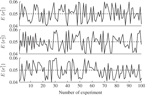
Figure 6.2 Angle between original and estimated eigenvector for residual subspace.
6.1.3 Maximum likelihood PCA for known 
Wentzell et al. (1997) introduced a maximum likelihood estimation (Aldrich 1997) for PCA under the assumption that ![]() is known. The maximum likelihood formulation, which is discussed in the next subsection, relies on the following formulation
is known. The maximum likelihood formulation, which is discussed in the next subsection, relies on the following formulation
where ![]() 1 is the likelihood of occurrence of the error vector
1 is the likelihood of occurrence of the error vector ![]() , if the error vector follows
, if the error vector follows ![]() . According to 2.2,
. According to 2.2, ![]() , Ξs = zs. With k and l being sample indices, it is further assumed that
, Ξs = zs. With k and l being sample indices, it is further assumed that ![]() . If a total of K samples of z0 are available, z0(1), … , z0(k), … , z0(K), the maximum likelihood objective function is given by
. If a total of K samples of z0 are available, z0(1), … , z0(k), … , z0(K), the maximum likelihood objective function is given by
where ![]() is defined by (6.18) when replacing z0 and zs with z0(k) and zs(k), respectively. The above function is a product of likelihood values that is larger than zero. As the logarithm function is monotonously increasing, taking the natural logarithm of J allows redefining (6.19)
is defined by (6.18) when replacing z0 and zs with z0(k) and zs(k), respectively. The above function is a product of likelihood values that is larger than zero. As the logarithm function is monotonously increasing, taking the natural logarithm of J allows redefining (6.19)
where J* = ln(J). Substituting (6.18) into (6.20) yields
Multiplying both sides by − 2 and omitting the constant terms 2Knzln(2π) and Kln(|Sgg|) gives rise to
where ![]() . A solution to the maximum likelihood objective function that is based on the reference set including K samples,
. A solution to the maximum likelihood objective function that is based on the reference set including K samples, ![]() , is the one that minimizes
, is the one that minimizes ![]() , which, in turn, maximizes J* and hence J. Incorporating the data model
, which, in turn, maximizes J* and hence J. Incorporating the data model ![]() , Fuller (1987) introduced an optimum solution for estimating the parameter matrix
, Fuller (1987) introduced an optimum solution for estimating the parameter matrix ![]()
that minimizes ![]() . Here:2
. Here:2
 ,
,  and
and  ;
; ;
; ; and
; and .
.
An iterative and efficient maximum likelihood PCA formulation based on a singular value decomposition for determining ![]() to minimize (6.22) was proposed by Wentzell et al. (1997). Reexamining (6.23) for
to minimize (6.22) was proposed by Wentzell et al. (1997). Reexamining (6.23) for ![]() suggests that the best linear unbiased estimate for
suggests that the best linear unbiased estimate for ![]() ,
, ![]() , is given by the generalized least squares solution of
, is given by the generalized least squares solution of ![]() (Björck 1996)
(Björck 1996)
In a PCA context, a singular value decomposition (SVD) of

where:
 ,
,  and
and  ; and
; and ,
,  and
and  ,
,
yields in its transposed form
where ![]() . Applying (6.24) to the above SVD produces
. Applying (6.24) to the above SVD produces
which can be simplified to
Equations (6.26) to (6.28) exploit the row space of Z0. Under the assumption that the error covariance matrix is of diagonal type, that is, no correlation among the error terms, the row space of Z0 can be rewritten with respect to (6.22)
6.29 
Analyzing the column space of ![]() , Equation (6.22) can alternatively be rewritten as
, Equation (6.22) can alternatively be rewritten as
The definition of the error covariance matrices in the above equations is
Equation (6.22) and the singular value decomposition of Z0 allow constructing a generalized least squares model for the column vectors of Z0
6.31 
Applying the same steps as those taken in (6.27) and (6.28) gives rise to
It should be noted that the error covariance matrix for the row space of Z0, ![]() , is the same for each row, which follows from the assumption made earlier that
, is the same for each row, which follows from the assumption made earlier that ![]() . However, the error covariance matrix for the column space or Z0 has different diagonal elements for each column. More precisely,
. However, the error covariance matrix for the column space or Z0 has different diagonal elements for each column. More precisely, ![]() which implies that (6.32) is equal to
which implies that (6.32) is equal to
6.33 ![]()
and hence
Using (6.28) and (6.34), the following iterative procedure computes a maximum likelihood PCA, or MLPCA, model:
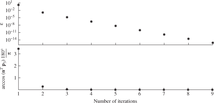
The performance of the iterative MLPCA approach is now tested for the three-variable example described in 2.9 and 2.11 and the error covariance matrix is defined in (6.14). Recall that the use of this error covariance matrix led to a biased estimation of the residual subspace, which departed from the true one by a minimum angle of almost 3.5°. The above MLPCA approach applied to a reference set of K = 1000 samples converged after nine times for a very tight threshold of 10−14. Figure 6.3 shows that after the first three iteration steps, the minimum angle between the true and estimated model subspaces is close to zero.
Figure 6.3 Convergence of the MLPCA algorithm for simulation example.
In contrast to the discussion above, it should be noted that the work in Wentzell et al. (1997) also discusses cases where the error covariance matrix is symmetric and changes over time. In this regard, the algorithms in Tables 1 and 2 respectively, in Wentzell et al. (1997) are of interest. The discussion in this book, however, assumes that the error covariance matrix remains constant over time.
6.1.4 Maximum likelihood PCA for unknown 
Different from the method proposed by Wentzell et al. (1997), Narasimhan and Shah (2008) introduced a more efficient method for determining an estimate of the model subspace. If the error covariance matrix is known a priori and of full rank, a Cholesky decomposition of ![]() can be obtained, which gives rise to
can be obtained, which gives rise to
with L being a lower triangular matrix. Rewriting (6.35) as follows
yields a transformed error covariance matrix ![]() that is of the type
that is of the type ![]() with
with ![]() . Hence, an eigendecomposition of
. Hence, an eigendecomposition of ![]() will provide a consistent estimation of the model subspace, which follows from (6.4) to (6.8). The dominant eigenvalues of
will provide a consistent estimation of the model subspace, which follows from (6.4) to (6.8). The dominant eigenvalues of ![]() are equal to the dominant eigenvalues of
are equal to the dominant eigenvalues of ![]() minus one, which the following relationship shows
minus one, which the following relationship shows
6.37 
By default, the diagonal elements of the matrices ![]() and
and ![]() are as follows
are as follows
Assuming that ![]() , it follows that
, it follows that
6.39 
and hence
6.40 
The determined eigenvectors of ![]() are consequently a consistent estimation of base vectors spanning the model subspace. Despite the strong theoretical foundation, conceptual simplicity and computational efficiency of applying an eigendecomposition to (6.36), it does not produce an estimate of the model subspace in a PCA sense, which Subsection 6.1.7 highlights.
are consequently a consistent estimation of base vectors spanning the model subspace. Despite the strong theoretical foundation, conceptual simplicity and computational efficiency of applying an eigendecomposition to (6.36), it does not produce an estimate of the model subspace in a PCA sense, which Subsection 6.1.7 highlights.
This approach, however, has been proposed by Narasimhan and Shah (2008) for developing an iterative approach that allows estimating ![]() under the constraint in (6.46), which is discussed below. Revising (6.1) and evaluating the stochastic components
under the constraint in (6.46), which is discussed below. Revising (6.1) and evaluating the stochastic components
6.41 ![]()
where ![]() , gives rise to
, gives rise to
Here ![]() is a matrix that has orthogonal rows to the columns in Ξ and hence
is a matrix that has orthogonal rows to the columns in Ξ and hence ![]() . Consequently, (6.42) reduces to
. Consequently, (6.42) reduces to
6.43 ![]()
The transformed error vector ![]() has therefore the distribution function
has therefore the distribution function
6.44 ![]()
since ![]() . Using the maximum likelihood function in (6.21) to determine
. Using the maximum likelihood function in (6.21) to determine ![]() leads to the following objective function to be minimized
leads to the following objective function to be minimized
It should be noted that the first term in (6.21), Knzln(2π) is a constant and can therefore be omitted. In contrast to the method in Wentzell et al. (1997), where the second term ![]() could be ignored, the log likelihood function for the approach by Narasimhan and Shah (2008) requires the inclusion of this term as
could be ignored, the log likelihood function for the approach by Narasimhan and Shah (2008) requires the inclusion of this term as ![]() is an unknown symmetric and positive definite matrix.
is an unknown symmetric and positive definite matrix.
Examining the maximum likelihood function of (6.45) or, more precisely, the error covariance matrix ![]() more closely, the rank of this matrix is nz − n and not nz. This follows from the fact that
more closely, the rank of this matrix is nz − n and not nz. This follows from the fact that ![]() . Consequently, the size of the model subspace is n and the number of linearly independent row vectors in
. Consequently, the size of the model subspace is n and the number of linearly independent row vectors in ![]() that are orthogonal to the column vectors in Ξ is nz − n. With this in mind,
that are orthogonal to the column vectors in Ξ is nz − n. With this in mind, ![]() and
and ![]() . This translates into a constraint for determining the number of elements in the covariance matrix as the maximum number of independent parameters is
. This translates into a constraint for determining the number of elements in the covariance matrix as the maximum number of independent parameters is ![]() .
.
Moreover, the symmetry of ![]() implies that only the upper or lower triangular elements must be estimated together with the diagonal ones. It is therefore imperative to constrain the number of estimated elements in
implies that only the upper or lower triangular elements must be estimated together with the diagonal ones. It is therefore imperative to constrain the number of estimated elements in ![]() . A practically reasonable assumption is that the errors are not correlated so that
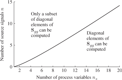
. A practically reasonable assumption is that the errors are not correlated so that ![]() reduces to a diagonal matrix. Thus, a complete set of diagonal elements can be obtained if (nz − n)(nz − n + 1) ≥ 2nz. The number of source signals must therefore not exceed
reduces to a diagonal matrix. Thus, a complete set of diagonal elements can be obtained if (nz − n)(nz − n + 1) ≥ 2nz. The number of source signals must therefore not exceed
Figure 6.4 illustrates that values for n must be below the graph ![]() for a determination of a complete set of diagonal elements for
for a determination of a complete set of diagonal elements for ![]() .
.
Figure 6.4 Graphical illustration of constraint in Equation (6.46).
Narasimhan and Shah (2008) introduced an iterative algorithm for simultaneously estimating the model subspace and ![]() from an estimate of
from an estimate of ![]() . This algorithm takes advantage of the fact that the model subspace and the residual space is spanned by the eigenvectors of
. This algorithm takes advantage of the fact that the model subspace and the residual space is spanned by the eigenvectors of ![]() . The relationship below proposes a slightly different version of this algorithm, which commences by defining the initial error covariance matrix that stores 0.0001 times the diagonal elements of
. The relationship below proposes a slightly different version of this algorithm, which commences by defining the initial error covariance matrix that stores 0.0001 times the diagonal elements of ![]() , then applies a Cholesky decomposition of
, then applies a Cholesky decomposition of ![]() and subsequently (6.36).
and subsequently (6.36).
Following an eigendecomposition of ![]()
6.47 
an estimate of ![]() is given by
is given by ![]() , which follows from the fact that column vectors of Ξ span the same column space as the eigenvectors in
, which follows from the fact that column vectors of Ξ span the same column space as the eigenvectors in ![]() after convergence. Given that
after convergence. Given that ![]() after convergence, it follows that
after convergence, it follows that
6.48 
Hence, ![]() and
and ![]() , since
, since ![]() . The next step is the evaluation of the objective function in (6.45) for
. The next step is the evaluation of the objective function in (6.45) for ![]() prior to an update of
prior to an update of ![]() ,
, ![]() , using a gradient projection method (Byrd et al. 1995), a genetic algorithm (Sharma and Irwin 2003) or a particle swarm optimization (Coello et al. 2004).
, using a gradient projection method (Byrd et al. 1995), a genetic algorithm (Sharma and Irwin 2003) or a particle swarm optimization (Coello et al. 2004).
Recomputing the Cholesky decomposition of ![]() then starts the (i + 1)th iteration step. The iteration converges if the difference of two consecutive values of
then starts the (i + 1)th iteration step. The iteration converges if the difference of two consecutive values of ![]() is smaller than a predefined threshold. Different to the algorithm in Narasimhan and Shah (2008), the proposed objective function here is of the following form
is smaller than a predefined threshold. Different to the algorithm in Narasimhan and Shah (2008), the proposed objective function here is of the following form
where || · ||2 is the squared Frobenius norm of a matrix. The rationale behind this objective function is to ensure that the solution found satisfies the following constraints
6.50 ![]()
Note that Subsection 6.1.7 elaborates upon the geometric relationships, such as ![]() in more detail. Since
in more detail. Since ![]() is orthogonal to the estimate of the model subspace, the following must hold true after the above iteration converged
is orthogonal to the estimate of the model subspace, the following must hold true after the above iteration converged
and
which is the second and third term in the objective function of (6.49). The coefficients a1, a2 and a3 influence the solution and may need to be adjusted if the solution violates at least one of the above constraints or the value of the first term appears to be too high. Enforcing that the solution meets the constraints requires larger values for a2 and a3, which the simulation example below highlights. The steps of the above algorithm are now summarized below.
To demonstrate the performance of the above algorithm, the next subsection presents an example. Section 6.2 describes a similar maximum likelihood algorithm for PLS models that relies on the inclusion of an additional error term for the input variables.
6.1.5 A simulation example
The three-variable example used previously in this chapter cannot be used here since three variables and two source signals leave only one parameter of ![]() to be estimated. The process studied here contains 14 variables that are described by the data model
to be estimated. The process studied here contains 14 variables that are described by the data model
where ![]() ,
, ![]() ,
, ![]()
and, ![]()
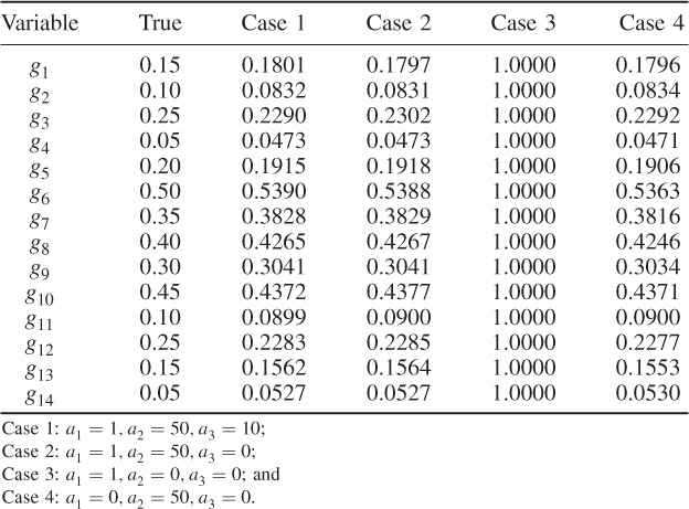
Recording 1000 samples from this process, setting the parameters for ![]() to be
to be
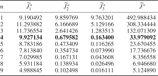
and the boundaries for the 14 diagonal elements to be ![]() , produced the results summarized in Tables 6.1 to 6.4 for Cases 1 to 4, respectively. Each table contains the resultant minimum of the objective function in (6.49), and the values for each of the three terms,
, produced the results summarized in Tables 6.1 to 6.4 for Cases 1 to 4, respectively. Each table contains the resultant minimum of the objective function in (6.49), and the values for each of the three terms, ![]() ,
, ![]() and
and ![]() for the inclusion of one to nine source signals. Note that n = 9 is the largest number that satisfies (6.46).
for the inclusion of one to nine source signals. Note that n = 9 is the largest number that satisfies (6.46).
Table 6.1 Results for a1 = 1, a2 = 50, a3 = 10.
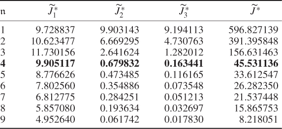
Table 6.2 Results for a1 = 1, a2 = 50, a3 = 0.
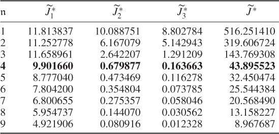
Table 6.3 Results for a1 = 1, a2 = 0, a3 = 0.
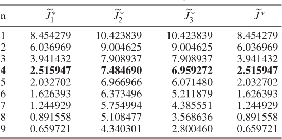
Table 6.4 Results for a1 = 0, a2 = 50, a3 = 0.
The results were obtained using the constraint nonlinear minimization function ‘fmincon’ of the MatlabTM optimization toolbox, version 7.11.0.584 (R2010b). The results for Cases 1 and 2 do not differ substantially. This follows from the supplementary character of the constraints, which (6.51) and (6.52) show
6.56 
Selecting a large a2 value for the second term in (6.49) addresses the case of small discarded eigenvalues for ![]() and suggests that the third term may be removed. Its presence, however, balances between the second and third terms and circumvents a suboptimal solution for larger process variable sets that yields discarded eigenvalues which are close to 1 but may not satisfy the 3rd constraint.
and suggests that the third term may be removed. Its presence, however, balances between the second and third terms and circumvents a suboptimal solution for larger process variable sets that yields discarded eigenvalues which are close to 1 but may not satisfy the 3rd constraint.
That Case 3 showed a poor performance is not surprising given that the only contributor to the first term is ![]() . To produce small values in this case, the diagonal elements of
. To produce small values in this case, the diagonal elements of ![]() need to be small, which, in turn, suggests that larger error variance values are required. A comparison of the estimated error variances in Table 6.5 confirms this and stresses that the case of minimizing the log likelihood function only is insufficient for estimating the error covariance matrix.
need to be small, which, in turn, suggests that larger error variance values are required. A comparison of the estimated error variances in Table 6.5 confirms this and stresses that the case of minimizing the log likelihood function only is insufficient for estimating the error covariance matrix.
Table 6.5 Resultant estimates for ![]() .
.
Another interesting observation is that Case 4 (Table 6.4) produced a small value for the objective function after four components were retained. In fact, Table 6.5 highlights that the selection of the parameters for Case 4 produced a comparable accuracy in estimating the diagonal elements ![]() . This would suggest omitting the contribution of the log likelihood function to the objective function and concentrating on terms two and three only. Inspecting Table 6.5 supports this conclusion, as most of the error variances are as accurately estimated as in Cases 1 and 2. However, the application for larger variable sets may yield suboptimal solutions, which the inclusion of the first term, the objective function in Equation (6.49), may circumvent.
. This would suggest omitting the contribution of the log likelihood function to the objective function and concentrating on terms two and three only. Inspecting Table 6.5 supports this conclusion, as most of the error variances are as accurately estimated as in Cases 1 and 2. However, the application for larger variable sets may yield suboptimal solutions, which the inclusion of the first term, the objective function in Equation (6.49), may circumvent.
It is not only important to estimate ![]() accurately but also to estimate the model subspace consistently, which has not been looked at thus far. The simplified analysis in (6.17) for nz = 3 and n = 2 cannot, of course, be utilized in a general context. Moreover, the column space of Ξ can only be estimated up to a similarity transformation, which does not allow a comparison of the column vectors either.
accurately but also to estimate the model subspace consistently, which has not been looked at thus far. The simplified analysis in (6.17) for nz = 3 and n = 2 cannot, of course, be utilized in a general context. Moreover, the column space of Ξ can only be estimated up to a similarity transformation, which does not allow a comparison of the column vectors either.
The residual subspace is orthogonal to Ξ, which allows testing whether the estimated residuals subspace, spanned by the column vectors of ![]() , is perpendicular to the column space in Ξ. If so,
, is perpendicular to the column space in Ξ. If so, ![]() asymptotically converges to 0. Using
asymptotically converges to 0. Using ![]() , obtained for a1 = 1, a2 = 50 and a3 = 10 this product is
, obtained for a1 = 1, a2 = 50 and a3 = 10 this product is
6.57 
The small values in the above matrix indicate an accurate estimation of the model and residual subspace by the MLPCA algorithm. A comparison of the accuracy of estimating the model subspace by the MLPCA model with that of the PCA model yields, surprisingly, very similar results. More precisely, the matrix product ![]() , where
, where ![]() stores the last 10 eigenvectors of
stores the last 10 eigenvectors of ![]() , is equal to
, is equal to
6.58 
Increasing the error variance and the differences between the individual elements as well as the number of reference samples, however, will increase the difference between both estimates. A detailed study regarding this issue is proposed in the tutorial session of this chapter (Project 1). It is also important to note that PCA is unable to provide estimates of the error covariance matrix. To demonstrate this Figure 6.5 shows the distribution of eigenvalues of ![]() .
.
Figure 6.5 Plot of eigenvalues of ![]() .
.
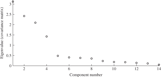
The next section introduces a stopping rule for MLPCA models. It is interesting to note that applying this rule for determining n yields a value of 1601.293 for (6.59), whilst the threshold is 85.965. This would clearly reject the hypothesis that the discarded 10 eigenvalues are equal. In fact, the application of this rule would not identify any acceptable value for ![]() .
.
6.1.6 A stopping rule for maximum likelihood PCA models
Most stopping rules summarized in Subsection 2.4.1 estimate n based on the assumption that ![]() or analyze the variance of the recorded samples projected onto the residuals subspace. The discussion in this section, however, has outlined that the model subspace is only estimated consistently for
or analyze the variance of the recorded samples projected onto the residuals subspace. The discussion in this section, however, has outlined that the model subspace is only estimated consistently for ![]() , which requires a different stopping rule for estimating n.
, which requires a different stopping rule for estimating n.
Feital et al. (2010) introduced a stopping rule if ![]() . This rule relies on a hypothesis for testing the equality of the discarded eigenvalues. Equations (6.36) and (6.38) outline that these eigenvalues are 1 after applying the Cholesky decomposition to
. This rule relies on a hypothesis for testing the equality of the discarded eigenvalues. Equations (6.36) and (6.38) outline that these eigenvalues are 1 after applying the Cholesky decomposition to ![]() . To test whether the nz − n discarded eigenvalues are equal, Section 11.7.3 in Anderson (2003) presents the following statistic, which has a limiting χ2 distribution with
. To test whether the nz − n discarded eigenvalues are equal, Section 11.7.3 in Anderson (2003) presents the following statistic, which has a limiting χ2 distribution with ![]() degrees of freedom
degrees of freedom
It should be noted that the estimated eigenvalues ![]() are those of the scaled covariance matrix
are those of the scaled covariance matrix ![]() . According to the test statistic in (6.59), the null hypothesis is that the
. According to the test statistic in (6.59), the null hypothesis is that the ![]() eigenvalues are equal. The alternative hypothesis is that the discarded
eigenvalues are equal. The alternative hypothesis is that the discarded ![]() eigenvalues are not identical and
eigenvalues are not identical and ![]() .
.
The critical value of the χ2 distribution for a significance α depends on the number of degrees of freedom for the χ2 distribution. The statistic κ2 must be compared against the critical value for ![]() , where dof represents the number of degrees of freedom. The null hypothesis H0 is therefore accepted if
, where dof represents the number of degrees of freedom. The null hypothesis H0 is therefore accepted if
6.60 ![]()
and rejected if
6.61 ![]()
While H0 describes the equality of the discarded nz − n eigenvalues, H1 represents the case of a statistically significant difference between these eigenvalues.
The formulation of the stopping rule is therefore as follows. Start with ![]() and obtain an MLPCA model. Then, compute the κ2 value for (6.59) along with the critical value of a χ2 distribution for
and obtain an MLPCA model. Then, compute the κ2 value for (6.59) along with the critical value of a χ2 distribution for ![]() degrees of freedom and a significance of α. Accepting H0 yields n = 1 and this model includes the estimate of the model subspace
degrees of freedom and a significance of α. Accepting H0 yields n = 1 and this model includes the estimate of the model subspace ![]() and its orthogonal complement
and its orthogonal complement ![]() . For rejecting H0, iteratively increment
. For rejecting H0, iteratively increment ![]() ,
, ![]() , compute a MLPCA model and test H0 until
, compute a MLPCA model and test H0 until ![]() .
.
To simplify the iterative sequence of hypothesis tests, κ2 can be divided by ![]()
which gives rise to the following formulation of the stopping rule
and
6.64 ![]()
The introduction of the stopping rule is now followed by an application study to the simulated process described in (6.53) to (6.55). This requires the application of (6.59), (6.62) and (6.63) to the MLPCA model for a varying number of estimated source signals, starting from 1. Table 6.6 shows the results of this series of hypothesis tests for ![]() for a significance of α = 0.05.
for a significance of α = 0.05.
Table 6.6 Results for estimating n.
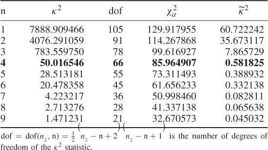
The results in Table 6.6 confirm that ![]() for
for ![]() . For
. For ![]() , the null hypothesis is accepted and hence, the ten discarded eigenvalues are equivalent. Increasing
, the null hypothesis is accepted and hence, the ten discarded eigenvalues are equivalent. Increasing ![]() further up to
further up to ![]() also yields equivalent eigenvalues, which is not surprising either. For the sequence of nine hypothesis tests in Table 6.6, it is important to note that the first acceptance of H0 is the estimate for n.
also yields equivalent eigenvalues, which is not surprising either. For the sequence of nine hypothesis tests in Table 6.6, it is important to note that the first acceptance of H0 is the estimate for n.
6.1.7 Properties of model and residual subspace estimates
After introducing how to estimate the column space of Ξ and its complementary residual subspace ![]() , the next question is what are the geometric properties of these estimates. The preceding discussion has shown that the estimates for column space of Ξ, the generalized inverse5 and its orthogonal complement are
, the next question is what are the geometric properties of these estimates. The preceding discussion has shown that the estimates for column space of Ξ, the generalized inverse5 and its orthogonal complement are
where ![]() ,
, ![]() and
and ![]() store the n and the remaining nz − n eigenvectors of
store the n and the remaining nz − n eigenvectors of ![]() associated with eigenvalues larger than 1 and equal to 1, respectively.
associated with eigenvalues larger than 1 and equal to 1, respectively.
The missing proofs of the relationships in (6.65) are provided next, which commences by reformulating the relationship between the known covariance matrices of the recorded data vector, the uncorrupted data vector and the error vector
For simplicity, it is assumed that each of the covariance matrices are available. Carrying out the eigendecomposition of ![]() and comparing it to the right hand side of (6.66) gives rise to
and comparing it to the right hand side of (6.66) gives rise to
Pre- and post-multiplying (6.67) by L and LT yields
6.68 ![]()
It follows from (6.9) to (6.11) that the column space of Ξ is given by ![]() . With regards to (6.65),
. With regards to (6.65), ![]() is the orthogonal complement of Ξ, since
is the orthogonal complement of Ξ, since
6.69 ![]()
Finally, that ![]() is the generalized inverse of
is the generalized inverse of ![]() follows from
follows from
6.70 ![]()
Geometrically, the estimate Ξ and its orthogonal complement ![]() are estimates of the model and residual subspaces, respectively. The generalized inverse Ξ† and the orthogonal complement
are estimates of the model and residual subspaces, respectively. The generalized inverse Ξ† and the orthogonal complement ![]() allow the estimation of linear combinations of the source signals and linear combinations of the error variables, respectively, since
allow the estimation of linear combinations of the source signals and linear combinations of the error variables, respectively, since
With regards to (6.71), there is a direct relationship between the source signals and the components determined by the PCA model in the noise-free case
6.72 ![]()
For the case ![]() , it follows that
, it follows that
6.73 
Despite the fact that the source signals could be recovered for ![]() and approximated for
and approximated for ![]() and
and ![]() , the following two problems remain.
, the following two problems remain.
- the loading vectors point in directions that produce a maximum variance for each score variable; and
- the loading vectors may not have unit length.
In addition to the above points, Feital et al. (2010) highlighted that the score variables may not be statistically independent either, that is, the score vectors may not be orthogonal as is the case for PCA. This is best demonstrated by comparing the score variables computed by applying the generalized inverse ![]()
with those determined by an eigendecomposition of ![]()
Removing the impact of the error covariance matrix from (6.74) allows a direct comparison with (6.75)
which yields:
- that it generally cannot be assumed that the eigenvectors of
 are equal to those of
  ; and
; and - that it can also generally not be assumed that the eigenvalues of
 are equal to those of
The subscript s in (6.75) and (6.76) refers to the source signals. Finally, the matrix product ![]() is only a diagonal matrix if
is only a diagonal matrix if ![]() is diagonal and hence, L is of diagonal type.
is diagonal and hence, L is of diagonal type. ![]() , however, is assumed to be diagonal in (6.46). In any case, the row vectors in
, however, is assumed to be diagonal in (6.46). In any case, the row vectors in ![]() do not have unit length, as the elements in
do not have unit length, as the elements in ![]() are not generally 1. Moreover, if
are not generally 1. Moreover, if ![]() is not a diagonal matrix,
is not a diagonal matrix, ![]() does not, generally, have orthogonal column vectors.
does not, generally, have orthogonal column vectors.
Feital et al. (2010) and Ge et al. (2011) discussed two different methods for determining loading vectors of unit length that produce score variables that have a maximum variance, and are statistically independent irrespective of whether ![]() is a diagonal matrix or not. The first method has been proposed in Hyvarinen (1999); Yang and Guo (2008) and is to determine the eigendecomposition of
is a diagonal matrix or not. The first method has been proposed in Hyvarinen (1999); Yang and Guo (2008) and is to determine the eigendecomposition of ![]() , which yields the loading vectors stored in P. It is important to note, however, that the eigenvalues of
, which yields the loading vectors stored in P. It is important to note, however, that the eigenvalues of ![]() are not those of the computed score variables.
are not those of the computed score variables.
This issue has been addressed in Feital et al. (2010) by introducing a constraint NIPALS algorithm. Table 6.7 summarizes an algorithm similar to that proposed in Feital et al. (2010). This algorithm utilizes the estimated model subspace, spanned by the column vectors of ![]() under the assumption that
under the assumption that ![]() is of diagonal type.
is of diagonal type.
Table 6.7 Constraint NIPALS algorithm
| Step | Description | Equation |
| 1 | Initiate iteration | i = 1, Z(1) = Z0 |
| 2 | Set up projection matrix | |
| 3 | Define initial score vector | 0ti = Z(i)(:, 1) |
| 4 | Determine loading vector | |
| 5 | Scale loading vector | |
| 6 | Calculate score vector | |
| 7 | Compute eigenvalue | λi = ||1ti||2 |
| If ||1ti − 0ti|| > ε , set | ||
| 8 | Check for convergence | 0ti = 1ti and go to Step 4 else |
| set |
||
| 9 | Scale eigenvalue | |
| 10 | Deflate data matrix | |
| If i < n set i = i + 1 | ||
| 11 | Check for dimension | and go to Step 3 else |
| terminate iteration procedure |
In order to outline the working of this algorithm, setting ![]() in Step 2 reduces the algorithm in Table 6.7 to the conventional NIPALS algorithm (Geladi and Kowalski 1986). The conventional algorithm, however, produces an eigen-decomposition of
in Step 2 reduces the algorithm in Table 6.7 to the conventional NIPALS algorithm (Geladi and Kowalski 1986). The conventional algorithm, however, produces an eigen-decomposition of ![]() and the associated score vectors for Z0.
and the associated score vectors for Z0.
Setting ![]() , however, forces the eigenvectors to lie within the estimated model subspace. To see this, the following matrix projects any vector of dimension nz to lie within the column space of
, however, forces the eigenvectors to lie within the estimated model subspace. To see this, the following matrix projects any vector of dimension nz to lie within the column space of ![]() (Golub and van Loan 1996)
(Golub and van Loan 1996)
Lemma 2.1.1 and particularly 2.5 in Section 2.1 confirm that (6.77) projects any vector orthogonally onto the model plane. Figure 2.2 gives a schematic illustration of this orthogonal projection. Step 4 in Table 6.7, therefore, guarantees that the eigenvectors of ![]() lie in the column space of
lie in the column space of ![]() .
.
Step 5 ensures that the loading vectors are of unit length, whilst Step 6 records the squared length of the t-score vector, which is K − 1 times its variance since the samples stored in the data matrix have been mean centered. Upon convergence, Step 9 determines the variance of the ith score vector and Step 10 deflates the data matrix. It is shown in Section 9.1 that the deflation procedure gives rise to orthonormal p-loading vectors and orthogonal t-score vectors, and that the power method converges to the most dominant eigenvector (Golub and van Loan 1996).
The working of this constraint NIPALS algorithm is now demonstrated using data from the simulation example in Subsection 6.1.5. Subsection 6.1.8 revisits the application study of the chemical reaction process in Chapter 4 by identifying an MLPCA model including an estimate of the number of source signals and a rearrangement of the loading vectors by applying the constraint NIPALS algorithm.
6.1.7.1 Application to data from the simulated process in subsection 6.1.5
By using a total of K = 1000 simulated samples from this process and including n = 4 source signals, the application of MLPCA yields the following loading matrix
6.78 
Applying the constraint NIPALS algorithm, however, yields a different loading matrix
6.79 
Finally, taking the loading matrix obtained from the constraint NIPALS algorithm and comparing the estimated covariance matrix of the score variables
6.80 
with those obtained from the loading matrix determined from the original data covariance matrix, i.e. ![]() and
and ![]()
6.81 
yields that the diagonal elements that are very close to the theoretical maximum for conventional PCA. The incorporation of the constraint (Step 4 of the constraint NIPALS algorithm in Table 6.7) clearly impacts the maximum value but achieves:
- an estimated model subspace is that obtained from the MLPCA algorithm; and
- loading vectors that produce score variables which have a maximum variance.
6.1.8 Application to a chemical reaction process—revisited
To present a more challenging and practically relevant application study, this subsection revisits the application study of the chemical reaction process. Recall that the application of PCA relied on the following assumptions outlined in Section 2.1
 , where:
 ;
; ;
;- with i and j being two sample indices
![]()
- the covariance matrices Sss and
 have full rank n and nz, respectively.
Determining the number of source signals
Under these assumptions, the application of the VRE technique suggested that the data model has four source signals (Figure 4.4). Inspecting the eigenvalue plot in Figure 4.3, however, does not support the assumption that the remaining 31 eigenvalues have the same value even without applying (6.59) and carrying out the hypothesis test for H0 in (6.59) and (6.63).
According to (6.46), the maximum number of source signals for a complete estimation of the diagonal elements of ![]() is 27. Different to the suggested number of four source signals using the VRE criterion, the application of the hypothesis test in Subsection 6.1.6 yields a total of 20 source signals.
is 27. Different to the suggested number of four source signals using the VRE criterion, the application of the hypothesis test in Subsection 6.1.6 yields a total of 20 source signals.
Table 6.8 lists the results for estimating the MLPCA model, including the optimal value of the objective function in (6.49), ![]() , the three contributing terms,
, the three contributing terms, ![]() ,
, ![]() and
and ![]() , the κ2 values of (6.59), its number of degrees of freedom (dof) and its critical value
, the κ2 values of (6.59), its number of degrees of freedom (dof) and its critical value ![]() for
for ![]() = 1, … , 27.
= 1, … , 27.
Table 6.8 Estimation results for MLPCA model (chemical reaction process).
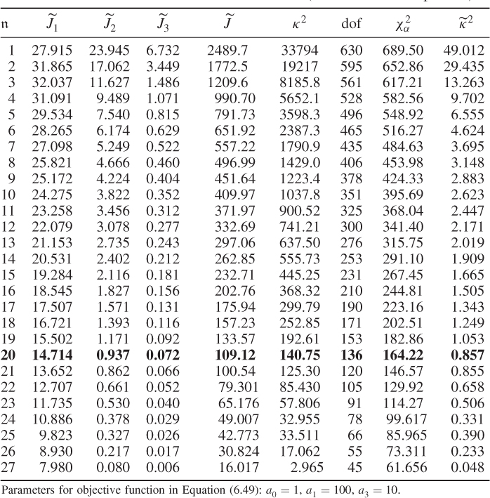
For (6.49), the diagonal elements of the error covariance matrix were constrained to be within ![]() , which related to the pretreatment of the data. Each temperature variable was mean centered and scaled to unity variance. Consequently, a measurement uncertainty of each thermocouples exceeding 50% of its variance was not expected and the selection of a too small lower boundary might have resulted in numerical problems in computing the inverse of the lower triangular matrix of the Cholesky decomposition, according to (6.36). The parameters for
, which related to the pretreatment of the data. Each temperature variable was mean centered and scaled to unity variance. Consequently, a measurement uncertainty of each thermocouples exceeding 50% of its variance was not expected and the selection of a too small lower boundary might have resulted in numerical problems in computing the inverse of the lower triangular matrix of the Cholesky decomposition, according to (6.36). The parameters for ![]() ,
, ![]() and
and ![]() were a1 = 1, a2 = 100 and a3 = 10, respectively.
were a1 = 1, a2 = 100 and a3 = 10, respectively.
Table 6.9 lists the elements of ![]() for n = 20. It should be noted that most error variances are between 0.05 and 0.13 with the exception of thermocouple 22 and 24. When comparing the results with PCA, the estimated model subspace for MLPCA is significantly larger. However, the application of MLPCA has shown here that estimating the model subspace simply by computing the eigendecomposition of
for n = 20. It should be noted that most error variances are between 0.05 and 0.13 with the exception of thermocouple 22 and 24. When comparing the results with PCA, the estimated model subspace for MLPCA is significantly larger. However, the application of MLPCA has shown here that estimating the model subspace simply by computing the eigendecomposition of ![]() has relied on an incorrect data structure. According to the results in Table 6.8, retaining just four PCs could not produce equal eigenvalues even under the assumption of unequal diagonal elements of
has relied on an incorrect data structure. According to the results in Table 6.8, retaining just four PCs could not produce equal eigenvalues even under the assumption of unequal diagonal elements of ![]() .
.
Table 6.9 Estimated diagonal elements of ![]() .
.
| Variable (diagonal | Error |
| element of |
variance |
| 0.0542 | |
| 0.1073 | |
| 0.0858 | |
| 0.0774 | |
| 0.0675 | |
| 0.0690 | |
| 0.0941 | |
| 0.0685 | |
| 0.0743 | |
| 0.0467 | |
| 0.1038 | |
| 0.0798 | |
| 0.0611 | |
| 0.0748 | |
| 0.0531 | |
| 0.1163 | |
| 0.0475 | |
| 0.0688 | |
| 0.0688 | |
| 0.0792 | |
| 0.0553 | |
| 0.0311 | |
| 0.1263 | |
| 0.2179 | |
| 0.0794 | |
| 0.0764 | |
| 0.0688 | |
| 0.0648 | |
| 0.0802 | |
| 0.0816 | |
| 0.0672 | |
| 0.0777 | |
| 0.0643 | |
| 0.0714 | |
| 0.0835 |
Chapter 4 discussed the distribution function of the source signals and showed that the first four score variables are, in fact, non-Gaussian. Whilst it was still possible to construct the Hotelling's T2 and Q statistics that were able to detect an abnormal behavior, the issue of non-Gaussian source signals is again discussed in Chapter 8. Next, the adjustment of the base vectors spanning the model subspace is considered.
Readjustment of the base vector spanning the model subspace
Table 6.10 lists the eigenvectors obtained by the constraint NIPALS algorithm. Table 6.11 shows the differences in the eigenvalues of ![]() and those obtained by the constraint NIPALS algorithm. Figure 6.6 presents a clearer picture for describing the impact of the constraint NIPALS algorithm. The first four eigenvalues and eigenvectors show a negligible difference but the remaining ones depart significantly by up to 90° for the eigenvectors and up to 10% for the eigenvalues.
and those obtained by the constraint NIPALS algorithm. Figure 6.6 presents a clearer picture for describing the impact of the constraint NIPALS algorithm. The first four eigenvalues and eigenvectors show a negligible difference but the remaining ones depart significantly by up to 90° for the eigenvectors and up to 10% for the eigenvalues.
Figure 6.6 Percentage change in angle of eigenvectors and eigenvalues.
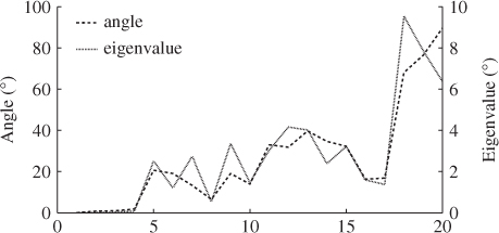
Table 6.10 Eigenvectors associated with first seven dominant eigenvalues
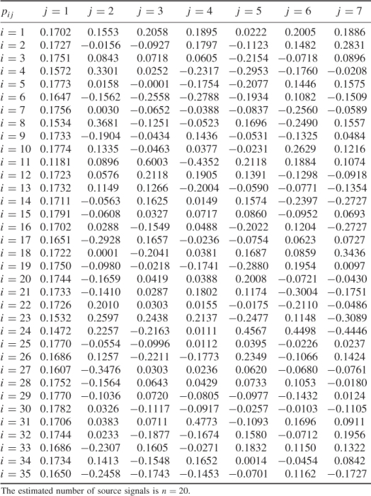
Table 6.11 Variances of score variables
| Component | Eigenvalue | Eigenvalue after |
| of |
adjustment | |
| 1 | 28.2959 | 28.2959 |
| 2 | 1.5940 | 1.5937 |
| 3 | 1.2371 | 1.2368 |
| 4 | 0.4101 | 0.4098 |
| 5 | 0.3169 | 0.3090 |
| 6 | 0.2981 | 0.2945 |
| 7 | 0.2187 | 0.2127 |
| 8 | 0.1929 | 0.1918 |
| 9 | 0.1539 | 0.1487 |
| 10 | 0.1388 | 0.1368 |
| 11 | 0.1297 | 0.1258 |
| 12 | 0.1251 | 0.1199 |
| 13 | 0.1199 | 0.1150 |
| 14 | 0.1148 | 0.1120 |
| 15 | 0.1067 | 0.1033 |
| 16 | 0.1015 | 0.0999 |
| 17 | 0.0980 | 0.0967 |
| 18 | 0.0939 | 0.0849 |
| 19 | 0.0919 | 0.0847 |
| 20 | 0.0884 | 0.0828 |
Summary of the application of MLPCA
Relying on the assumption that ![]() suggested a relatively low number of source signals. Removing the assumption, however, presented a different picture and yielded a significantly larger number of source signals. A direct inspection of Figure 4.3 confirmed that the discarded components do not have an equal variance and the equivalence of the eigenvalues for the MLPCA has been tested in a statistically sound manner. The incorporation of the identified model subspace into the determination of the eigendecomposition of
suggested a relatively low number of source signals. Removing the assumption, however, presented a different picture and yielded a significantly larger number of source signals. A direct inspection of Figure 4.3 confirmed that the discarded components do not have an equal variance and the equivalence of the eigenvalues for the MLPCA has been tested in a statistically sound manner. The incorporation of the identified model subspace into the determination of the eigendecomposition of ![]() yielded a negligible difference for the first four eigenvalues and eigenvectors but significant differences for the remaining 16 eigenpairs. This application study, therefore, shows the need for revisiting and testing the validity of the assumptions imposed on the data models. Next, we examine the performance of the revised monitoring statistics in detecting the abnormal behavior of Tube 11 compared to the monitoring model utilized in Chapter 4.
yielded a negligible difference for the first four eigenvalues and eigenvectors but significant differences for the remaining 16 eigenpairs. This application study, therefore, shows the need for revisiting and testing the validity of the assumptions imposed on the data models. Next, we examine the performance of the revised monitoring statistics in detecting the abnormal behavior of Tube 11 compared to the monitoring model utilized in Chapter 4.
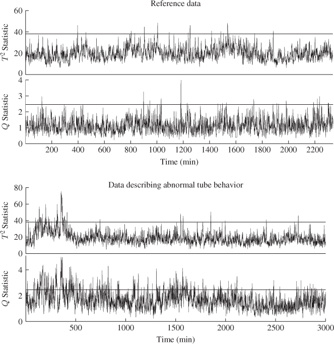
Detecting the abnormal behavior in tube 11
Figure 6.7 shows the Hotelling's T2 and Q statistics for both data sets. Comparing Figure 4.10 with the upper plots in Figure 6.7, outlines that the inclusion of a larger number set of source signals does not yield the same ‘distinct’ regions, for example between 800 to 1100 minutes and between 1400 and 1600 minutes into the data set.
Figure 6.7 MLPCA-based monitoring statistics.
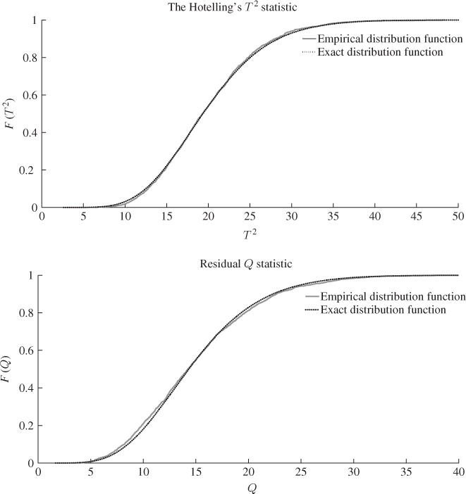
To qualify this observation, Figure 6.8 compares the F-distribution function with the empirical one, which shows a considerably closer agreement when contrasted with the PCA-based comparison in Figure 4.8. The upper plot in Figure 4.8 shows significant departures between the theoretical and the estimated distribution functions for the Hotelling's T2 statistic. In contrast, the same plot in Figure 6.8 shows a close agreement for the MLPCA-based statistic. The residual-based Q statistics for the PCA and MLPCA models are accurately approximated by an F-distribution, when constructed with respect to (3.20), that is, ![]() .
.
Figure 6.8 F-distribution (dotted line) and estimated distribution functions.
The reason that the MLPCA-based Hotelling's T2 statistic is more accurately approximated by an F-distribution with 2338 and 20 degrees of freedom than the PCA-based one by an F-distribution with 2338 and 4 degrees of freedom is as follows. Whilst the first four components are strongly non-Gaussian, the remaining ones show significantly smaller departures from a Gaussian distribution. Figure 6.9 confirms this by comparing the estimated distribution function with the Gaussian one for score variables 5, 10, 15 and 20. Moreover, the construction of the Hotelling's T2 statistic in 3.9 implies that each of the first four non-Gaussian score variables has the same contribution compared to the remaining 16 score variables. The strong impact of the first four highly non-Gaussian score variables to the distribution function of the Hotelling's T2 statistic therefore becomes reduced for n = 20.
Figure 6.9 Comparison between Gaussian distribution (dashed line) and estimated distribution function for score variables 5 (upper left plot), 10 (upper right plot), 15 (lower left plot) and 20 (lower right plot).

Analyzing the sensitivity of the MLPCA monitoring model in detecting the abnormal tube behavior requires comparing Figure 4.10 with the lower plots in Figure 6.7. This comparison yields a stronger response of both MLPCA-based non-negative squared monitoring statistics. In other words, the violation of the control limits, particularly by the MLPCA-Q statistic, is more pronounced. The inspection of Figure 4.17 highlights that the estimated fault signature for temperature variable #11 is not confined to the first third of the data set but instead spans over approximately two thirds of the recorded set. More precisely, the violation of the control limit by the MLPCA-based Q statistic corresponds more closely to the extracted fault signature.
In summary, the revised application study of the chemical reaction process outlined the advantage of MLPCA over PCA, namely a more accurate model estimation with respect to the data structure in 2.2. In contrast, the PCA model violated the assumption of ![]() . From the point of detecting the abnormal tube behavior, this translated into an increased sensitivity of both non-negative quadratic monitoring statistics by comparing Figures 4.12 and 6.7. Despite the increased accuracy in estimating a data model for this process, the problem that the first four score variables do not follow a Gaussian distribution remains. Chapter 8 introduces a different construction of monitoring statistics that asymptotically follow a Gaussian distribution irrespective of the distribution function of the individual process variables and, therefore, addresses this remaining issue.
. From the point of detecting the abnormal tube behavior, this translated into an increased sensitivity of both non-negative quadratic monitoring statistics by comparing Figures 4.12 and 6.7. Despite the increased accuracy in estimating a data model for this process, the problem that the first four score variables do not follow a Gaussian distribution remains. Chapter 8 introduces a different construction of monitoring statistics that asymptotically follow a Gaussian distribution irrespective of the distribution function of the individual process variables and, therefore, addresses this remaining issue.
6.2 Accuracy of estimating PLS models
This section discusses the accuracy of estimating the weight and loading vectors as well as the regression matrix of PLS models. In this regard, the issue of high degrees of correlation among and between the input and output variable sets is revisited. Section 6.2.1 first summarizes the concept of bias and variance in estimating a set of unknown parameters. Using a simulation example, Subsection 6.2.2 then demonstrates that high correlation can yield a considerable variance of the parameter estimation when using OLS and outlines that PLS circumvents this large variance by including a reduced set of LVs in the regression model (Wold et al. 1984).
This, again, underlines the benefits of using MSPC methods in this context, which decompose the variation encapsulated in the highly correlated variable sets into source signals and error terms. For the identification of suitable models for model predictive control application, this is also an important issue. A number of research articles outline that PLS can outperform OLS and other multivariate regression techniques such as PCR and CCR (Dayal and MacGregor 1997b; Duchesne and MacGregor 2001) unless specific penalty terms are included in regularized least square (Dayal and MacGregor 1996) which, however, require prior knowledge of how to penalize changes in the lagged parameters of the input variables.
Finally, Subsection 6.2.3 shows how to obtain a consistent estimation of the LV sets and the parametric regression matrix if the data structure is assumed to be ![]() , whilst
, whilst ![]() where
where ![]() is an error vector for the input variables.
is an error vector for the input variables.
6.2.1 Bias and variance of parameter estimation
According to 2.24 and 2.51, the number of source signals n must be smaller or equal to nx. It is important to note, however, that if n < nx a unique ordinary least squares solution for estimating ![]() ,
, ![]() , does not exist. More precisely, if n < nx the covariance matrix for the input variables is asymptotically ill conditioned and the linear equation
, does not exist. More precisely, if n < nx the covariance matrix for the input variables is asymptotically ill conditioned and the linear equation ![]() yields an infinite number of solutions. On the other hand, if the condition number of the estimated covariance matrix
yields an infinite number of solutions. On the other hand, if the condition number of the estimated covariance matrix ![]() is very large, the estimation variance of the elements in
is very large, the estimation variance of the elements in ![]() can become very large too. This is now analyzed in more detail.
can become very large too. This is now analyzed in more detail.
The OLS estimation is the best linear unbiased estimator if the error covariance matrix is of diagonal type ![]()
It is important to note the data structures in 2.24 and 2.51 do not include any stochastic error terms for the input variables. Although the input and, therefore, the uncorrupted output variables are also assumed to follow multivariate Gaussian distributions, the K observations are assumed to be known. Hence, the only unknown stochastic element in the above relationship is ![]() , which has an expectation of zero. Hence the OLS solution is unbiased.
, which has an expectation of zero. Hence the OLS solution is unbiased.
The next step is to examine the covariance matrix of the parameter estimation for each column vector of ![]() . For the ith column of
. For the ith column of ![]() , the corresponding covariance matrix can be constructed from
, the corresponding covariance matrix can be constructed from ![]() , which follows from (6.82)
, which follows from (6.82)
6.83 
which can be simplified to
It follows from the Isserlis theorem (Isserlis 1918), that
6.85 
Incorporating the fact that:
 ; and
; and if k = l
allows simplifying (6.84) to become (Ljung 1999)
That ![]() follows from the assumption that the error variables are independently distributed and do not possess any serial- or autocorrelation. Furthermore, the error variables are statistically independent of the input variables. At first glance, it is important to note that a large sample size results in a small variance for the parameter estimation.
follows from the assumption that the error variables are independently distributed and do not possess any serial- or autocorrelation. Furthermore, the error variables are statistically independent of the input variables. At first glance, it is important to note that a large sample size results in a small variance for the parameter estimation.
It is also important to note, however, that the condition number of the estimated covariance matrix ![]() has a significant impact upon the variance of the parameter estimation. To see this, using the eigendecomposition of
has a significant impact upon the variance of the parameter estimation. To see this, using the eigendecomposition of ![]() , its inverse becomes
, its inverse becomes ![]() . If there is at least one eigenvalue that is close to zero, some of elements of the inverse matrix become very large, since
. If there is at least one eigenvalue that is close to zero, some of elements of the inverse matrix become very large, since ![]() contains some large values which depend on the elements in nxth eigenvector
contains some large values which depend on the elements in nxth eigenvector ![]() .
.
With regards to the data structure in 2.24, PLS can provide an estimate of the parameter matrix that predicts the output variables y0 based on the t-score variables and hence circumvents the problem of a large estimation variance for determining the regression matrix ![]() using OLS. This is now demonstrated using a simulation example.
using OLS. This is now demonstrated using a simulation example.
6.2.2 Comparing accuracy of PLS and OLS regression models
The example includes one output variable and ten highly correlated input variables
where ![]() ,
, ![]() ,
, ![]() and
and ![]() . Furthermore, s and s′ are statistically independent, i.i.d. and follow a multivariate Gaussian distribution with diagonal covariance matrices. The diagonal elements of Sss and
. Furthermore, s and s′ are statistically independent, i.i.d. and follow a multivariate Gaussian distribution with diagonal covariance matrices. The diagonal elements of Sss and ![]() are 1 and 0.075, respectively. The output variable is a linear combination of the ten input variables and corrupted by an error variable
are 1 and 0.075, respectively. The output variable is a linear combination of the ten input variables and corrupted by an error variable
6.88 ![]()
The elements of the parameter matrices P and P′ as well as the parameter vector ![]() , shown in (6.89a) to (6.89c), were randomly selected to be within
, shown in (6.89a) to (6.89c), were randomly selected to be within ![]() from a uniform distribution. The variance of the error term was
from a uniform distribution. The variance of the error term was ![]() . It should be noted that the data structure in this example is different from that in 2.51, as both types of source signals influence the output variables.
. It should be noted that the data structure in this example is different from that in 2.51, as both types of source signals influence the output variables.
6.89a 
6.89b 
6.89c 
With respect to (6.87) to (6.89c), the covariance matrix of x0 is
Equation (6.86) shows that the variance of the parameter estimation for the OLS solution is proportional to ![]() but also depends on the estimated covariance matrix. With respect to the true covariance matrix in (6.90), it is possible to approximate the covariance matrix for the parameter estimation using OLS
but also depends on the estimated covariance matrix. With respect to the true covariance matrix in (6.90), it is possible to approximate the covariance matrix for the parameter estimation using OLS
6.91 ![]()
As discussed in the previous subsection, the examination of the impact of ![]() relies on its eigendecomposition
relies on its eigendecomposition
Given that the eigenvalues of ![]() are
are
6.93 
the condition number of ![]() is 2.9066 × 10⁵, which highlights that this matrix is indeed badly conditioned. On the basis of (6.92), Figure 6.10 shows the approximated variances for estimating the ten parameters, that is, the diagonal elements of
is 2.9066 × 10⁵, which highlights that this matrix is indeed badly conditioned. On the basis of (6.92), Figure 6.10 shows the approximated variances for estimating the ten parameters, that is, the diagonal elements of ![]() . The largest curves in Figure 6.10 are those for parameters
. The largest curves in Figure 6.10 are those for parameters ![]() ,
, ![]() ,
, ![]() ,
, ![]() (from largest to smallest). The remaining curves represent smaller but still significant variances for
(from largest to smallest). The remaining curves represent smaller but still significant variances for ![]() ,
, ![]() ,
, ![]() ,
, ![]() ,
, ![]() and
and ![]() . Even for a sample size of K = 1000, variances of the parameter estimation in the region of five can arise. The impact of such a large variance for the parameter estimation is now demonstrated using a Monte Carlo experiment.
. Even for a sample size of K = 1000, variances of the parameter estimation in the region of five can arise. The impact of such a large variance for the parameter estimation is now demonstrated using a Monte Carlo experiment.
Figure 6.10 Variance of parameter estimation (OLS model) for various sample sizes.

The experiment includes a sample size of K = 200 and a total number of 1000 repetitions. The comparison here is based on the parameter estimation using OLS and the estimation of latent variable sets using PLS. For each of these sets, the application of OLS and PLS produced estimates of the regression parameters and estimates of sets of LVs, respectively. Analyzing the 1000 estimated parameter sets for OLS and PLS then allow determining histograms of individual values for each parameter set, for example the OLS regression coefficients.
Figure 6.11 shows histograms for each of the ten regression parameters obtained using OLS. In each plot, the abscissa relates to the value of the estimated parameter and the ordinate shows the relative frequency of a particular parameter value. According to Figure 6.10, for K = 200, the largest estimation variance is in the region of 16 for the eighth parameter.
Figure 6.11 Histograms for parameter estimation of regression coefficients (OLS).
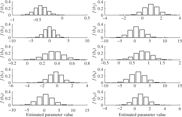
It follows from the central limit theorem that the parameter estimation follows approximately a Gaussian distribution with the mean value being the true parameter vector (unbiased estimation) and the covariance matrix given in (6.86). With this in mind, the estimated variance of 16 for the eighth parameter implies that around 68% of estimated parameters for ![]() are within the range 0.991 ± 4 and around 95% of estimated parameters fall in the range of 0.991 ± 8, which Figure 6.10 confirms.
are within the range 0.991 ± 4 and around 95% of estimated parameters fall in the range of 0.991 ± 8, which Figure 6.10 confirms.
The Monte Carlo simulation also shows larger variances for the parameter estimation for ![]() ,
, ![]() and
and ![]() . The ranges for estimating the remaining parameters, however, are still significant. For example, the smallest range is for estimating parameter
. The ranges for estimating the remaining parameters, however, are still significant. For example, the smallest range is for estimating parameter ![]() , which is bounded roughly by
, which is bounded roughly by ![]() . The above analysis therefore illustrates that the values of the parameter estimation can vary substantially and strongly depend on the recorded samples. Höskuldsson (1988) pointed out that PLS is to be preferred over OLS as it produces a more stable estimation of the regression parameters in the presence of highly correlated input variables. This is examined next.
. The above analysis therefore illustrates that the values of the parameter estimation can vary substantially and strongly depend on the recorded samples. Höskuldsson (1988) pointed out that PLS is to be preferred over OLS as it produces a more stable estimation of the regression parameters in the presence of highly correlated input variables. This is examined next.
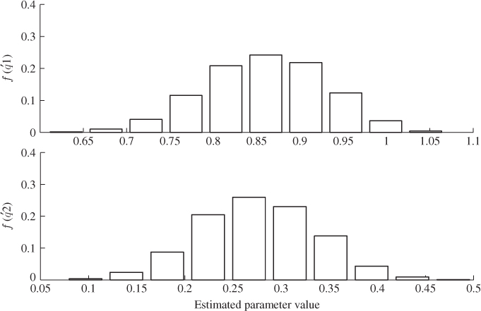
In contrast to OLS, PLS regression relates to an estimated parametric model between the extracted t-score and the output variables, ![]() . Figure 6.12, plotting the histograms for estimating the parameters of the first two q-loading values, does not show large variances for the parameter estimation. More precisely, the computed variance for the 1000 estimates of
. Figure 6.12, plotting the histograms for estimating the parameters of the first two q-loading values, does not show large variances for the parameter estimation. More precisely, the computed variance for the 1000 estimates of ![]() and
and ![]() are 0.0049 and 0.0038, respectively. Based on the original covariance matrix, constructed from the covariance matrix in (6.90) and
are 0.0049 and 0.0038, respectively. Based on the original covariance matrix, constructed from the covariance matrix in (6.90) and ![]() , the mean values for
, the mean values for ![]() and
and ![]() are 0.8580 and 0.2761, respectively. The estimation variance for
are 0.8580 and 0.2761, respectively. The estimation variance for ![]() and
and ![]() , therefore, compares favorably to the large estimation variances for
, therefore, compares favorably to the large estimation variances for ![]() , produced by applying OLS.
, produced by applying OLS.
Figure 6.12 Histograms for parameter estimation of ![]() -loading coefficients (PLS).
-loading coefficients (PLS).
The small estimation variance for the first and second ![]() -loading value, however, does not take into consideration the computation of the t-score variables. According to Lemma 10.4.7, the t-score variables can be obtained by the scalar product of the r-loading and the input variables, i.e.
-loading value, however, does not take into consideration the computation of the t-score variables. According to Lemma 10.4.7, the t-score variables can be obtained by the scalar product of the r-loading and the input variables, i.e. ![]() . For the first two r-loading vectors, Figure 6.13, again, suggests a small variance for each of the elements in r1 and r2, Table 6.12 lists the estimated mean and variance for each element of the two vectors. The largest variance is 0.0140 for element r52.
. For the first two r-loading vectors, Figure 6.13, again, suggests a small variance for each of the elements in r1 and r2, Table 6.12 lists the estimated mean and variance for each element of the two vectors. The largest variance is 0.0140 for element r52.
Figure 6.13 Histograms for parameter estimation of r-weight coefficients (PLS).
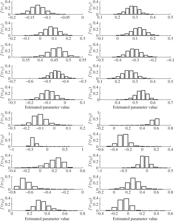
Table 6.12 Mean and variance for estimating r1 and r2.
| Element rij | ||
| r11 | −0.1261 | 0.0004 |
| r21 | 0.2859 | 0.0010 |
| r31 | 0.0782 | 0.0022 |
| r41 | 0.1196 | 0.0015 |
| r51 | 0.4576 | 0.0007 |
| r61 | −0.3060 | 0.0014 |
| r71 | −0.4498 | 0.0011 |
| r81 | 0.2664 | 0.0014 |
| r91 | −0.0913 | 0.0015 |
| r101 | 0.5341 | 0.0010 |
| r12 | −0.1001 | 0.0022 |
| r22 | 0.5645 | 0.0023 |
| r32 | −0.3861 | 0.0043 |
| r42 | −0.2651 | 0.0058 |
| r52 | 0.2000 | 0.0140 |
| r62 | −0.0472 | 0.0094 |
| r72 | −0.6329 | 0.0060 |
| r82 | 0.2816 | 0.0090 |
| r92 | 0.3470 | 0.0060 |
| r102 | −0.0600 | 0.0059 |
Equation (10.60) shows that the PLS estimate for the parameter matrix ![]() is
is ![]() . Retaining the first two latent variable pairs, Figure 6.14 shows the histograms of the elements of the PLS regression vectors. In contrast to the histograms of the loading and weight vectors in Figures 6.12 and 6.13, respectively, the histograms in Figure 6.14 can be directly compared to those in Figure 6.11. As expected, the variance of the parameter estimation for models obtained using PLS is significantly smaller compared to those computed by OLS. This is a result of the relatively small variance of the parameter estimation for the latent loading and weight vectors.
. Retaining the first two latent variable pairs, Figure 6.14 shows the histograms of the elements of the PLS regression vectors. In contrast to the histograms of the loading and weight vectors in Figures 6.12 and 6.13, respectively, the histograms in Figure 6.14 can be directly compared to those in Figure 6.11. As expected, the variance of the parameter estimation for models obtained using PLS is significantly smaller compared to those computed by OLS. This is a result of the relatively small variance of the parameter estimation for the latent loading and weight vectors.
Figure 6.14 Histograms for parameter estimation of regression coefficients (PLS).

A more qualitative analysis is offered in Table 6.13. It is interesting to note that the estimation using OLS is more accurate for parameter ![]() , which follows from the fact that the confidence region of this parameter, obtained from the estimates in Table 6.13 for a significance of 0.05, is
, which follows from the fact that the confidence region of this parameter, obtained from the estimates in Table 6.13 for a significance of 0.05, is ![]() 6 for OLS, which compares to − 0.2774 ± 0.0297 for the PLS models. In the worst case, the estimated parameter for OLS becomes 0.2390 for OLS, whilst the closest estimate for PLS is −0.2477. For almost all other parameters, the confidence regions for the estimated parameters using OLS include those of the PLS estimates. This is known as the bias/variance tradeoff, where an estimation bias by the regression tool is accepted in favor of a significantly reduced estimation variance.
6 for OLS, which compares to − 0.2774 ± 0.0297 for the PLS models. In the worst case, the estimated parameter for OLS becomes 0.2390 for OLS, whilst the closest estimate for PLS is −0.2477. For almost all other parameters, the confidence regions for the estimated parameters using OLS include those of the PLS estimates. This is known as the bias/variance tradeoff, where an estimation bias by the regression tool is accepted in favor of a significantly reduced estimation variance.
Table 6.13 Comparing accuracy of OLS and PLS regression models
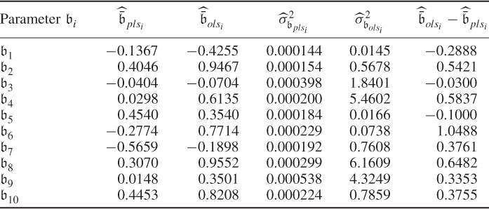
The application of PLS in this Monte Carlo study yielded, therefore, a better estimation of the parameters apart from ![]() with the retention of just two sets of latent variables compared to the application of OLS. Given that the PLS regression model is identical to the OLS regression model if all of the nx LV sets are included, increasing
with the retention of just two sets of latent variables compared to the application of OLS. Given that the PLS regression model is identical to the OLS regression model if all of the nx LV sets are included, increasing ![]() , consequently, reduces the estimation bias. On the other hand, the increase in
, consequently, reduces the estimation bias. On the other hand, the increase in ![]() significantly increases the variance of the parameter estimation.
significantly increases the variance of the parameter estimation.
Whilst the retention of only two latent variable sets yielded a biased parameter estimation that resulted in a substantial reduction in the variance of the estimation and hence, a more accurate parameter estimation, the final question is how accurate is the prediction of this model. Using the variance of the error term over the variance of the output variable as a measure of accuracy
Figure 6.15 indicates that including just one set of latent variables, the estimated mean value of the statistic in (6.94) for the PLS regression models is 0.2528 and 0.1289 if ![]() . For the retention of further latent variable sets, the estimated mean for this statistic becomes 0.1205, 0.1127, 0.0742, 0.0736, 0.0733, 0.0732, 0.0731, 0.0730. As analyzed above, however, an increase in
. For the retention of further latent variable sets, the estimated mean for this statistic becomes 0.1205, 0.1127, 0.0742, 0.0736, 0.0733, 0.0732, 0.0731, 0.0730. As analyzed above, however, an increase in ![]() will reduce the accuracy of the parameter estimation, whilst increasing the predictive performance of the resulting regression model for the reference data. A further study of this example is encouraged in the tutorial session of this chapter (Project 3).
will reduce the accuracy of the parameter estimation, whilst increasing the predictive performance of the resulting regression model for the reference data. A further study of this example is encouraged in the tutorial session of this chapter (Project 3).
Figure 6.15 Histograms of accuracy of PLS models for retaining ![]() .
.
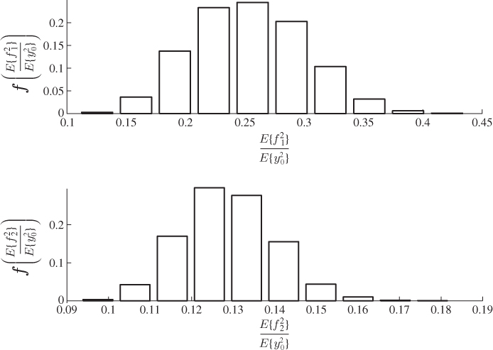
6.2.3 Impact of error-in-variables structure upon PLS models
After outlining the benefits of utilizing PLS as a technique for determining regression parameters in the presence of highly correlated input variables, we now focus on the accuracy of estimating the latent variable sets if the input variables are also corrupted by an error vector. Recall that the data structures in 2.24 and 2.51 only include the error term ![]() for the output variables. Such extended data structures are often referred to as error-in-variable or EIV structures (Söderström 2007).
for the output variables. Such extended data structures are often referred to as error-in-variable or EIV structures (Söderström 2007).
Error-in-variable data structure for PLS models
Equations (6.95) and (6.96) introduce the extended EIV data structures for PLS and MRPLS models, respectively, that include the error vector ![]() for the input variables
for the input variables

The following assumptions are imposed on ![]() ,
, ![]() ,
, ![]() and
and ![]()
6.97 ![]()
Defining k and l as sampling indices, the joint covariance matrix is assumed to be
6.98 
The data structure in (6.95) does not include s′. In this case, the covariance matrix of the joint variable sets only includes the stochastic vectors s, ![]() and
and ![]() . Moreover, the following linear parametric relationship exists between the ys and xs
. Moreover, the following linear parametric relationship exists between the ys and xs
The next few pages examine the impact of ![]() upon the computation of the LVs, commencing with the influence upon the covariance and cross-covariance matrices. Subsections 6.2.4 and 6.2.5 then discuss how to remove this undesired impact.
upon the computation of the LVs, commencing with the influence upon the covariance and cross-covariance matrices. Subsections 6.2.4 and 6.2.5 then discuss how to remove this undesired impact.
Impact upon  and
and 
The examination of the impact of ![]() upon the accuracy of the weight and loading vectors requires studying the impact of
upon the accuracy of the weight and loading vectors requires studying the impact of ![]() upon the covariance matrix
upon the covariance matrix ![]() and the cross-covariance matrix
and the cross-covariance matrix ![]() first. According to the data structures in (6.95) and (6.96), the covariance and cross-covariance matrices are given by
first. According to the data structures in (6.95) and (6.96), the covariance and cross-covariance matrices are given by
6.100 ![]()
With PLS being an iterative algorithm, the analysis commences with the first set of weight and loading vectors. It is important to note that a linear parametric relationship between xs and ys can be established irrespective of whether xs = Ps or xs = Ps + P′s′, provided that ![]() has full rank, which (6.99) shows.
has full rank, which (6.99) shows.
Impact on first set of weight vectors
This set of weight vectors is the solution to the following objective function
6.101 ![]()
which confirms that the inclusion of ![]() does not affect the first set of weight vectors.
does not affect the first set of weight vectors.
Impact on first set of loading vectors
Equation (6.102) shows the calculation of the first pair of loading vectors
which directly follows from 10.12 in Subsection 10.2. Compared to the analysis for the weight vector, however, a different picture emerges when analyzing the objective function in (6.102), since
where ![]() is the covariance matrix of the source signals, that is, without the inclusion of
is the covariance matrix of the source signals, that is, without the inclusion of ![]() . Without the presence of this term, the first pair of loading vectors are equal to
. Without the presence of this term, the first pair of loading vectors are equal to
6.104 ![]()
Here, the superscript * refers to the loading vectors determined from ![]() . The difference between the two pairs of loading vectors is therefore
. The difference between the two pairs of loading vectors is therefore
6.105 ![]()
and
where ![]() , since both covariance matrices are symmetric and positive definite. Equations (6.103) to (6.106) highlight that:
, since both covariance matrices are symmetric and positive definite. Equations (6.103) to (6.106) highlight that:
by the presence of ![]() . The reduction in length of the
. The reduction in length of the ![]() -loading vector follows from the fact that
-loading vector follows from the fact that ![]() is a symmetric and positive definite matrix of rank nx. Moreover, the scalar product
is a symmetric and positive definite matrix of rank nx. Moreover, the scalar product ![]() , which follows from Lemma 10.4.10 irrespective of whether the input variables are corrupted by the noise term or not. Consequently, the scalar product
, which follows from Lemma 10.4.10 irrespective of whether the input variables are corrupted by the noise term or not. Consequently, the scalar product ![]() . In other words,
. In other words, ![]() .
.
Impact upon deflation of 
Using (6.103) and Theorem 10.4.6 shows that the deflation of the cross-covariance matrix can be expressed as follows
6.107 ![]()
Given that the deflation of ![]() using the uncorrupted input variables is equal to
using the uncorrupted input variables is equal to
6.108 ![]()
the difference between ![]() and
and ![]() becomes
becomes
Impact on subsequent pairs of weight and loading vectors
After deflating the cross-covariance matrix, w2, q2, p2 and ![]() can be computed. Different from w1 and q1, the computation of w2 and q2 is affected by
can be computed. Different from w1 and q1, the computation of w2 and q2 is affected by ![]() , as they are the dominant left and right singular vectors of
, as they are the dominant left and right singular vectors of ![]() (Kaspar and Ray 1993), which follows from (6.109). In summary, each of the subsequent sets of LVs differs in the presence of the additional error term.
(Kaspar and Ray 1993), which follows from (6.109). In summary, each of the subsequent sets of LVs differs in the presence of the additional error term.
Impact upon regression model
Theorem 10.4.15 highlights that the identified parameter matrix is equal to the OLS estimate if all nx LV sets are included. The asymptotic OLS estimate is given by
6.110 ![]()
and for uncorrupted input variables
6.111 ![]()
The estimation bias is therefore
6.112 
The above relationship relies on the application of the matrix-inversion lemma, i.e. ![]() .
.
The analysis in (6.102) to (6.109) also applies for the MRPLS. However, the MRPLS cost function for determining the weight vectors is equal to
6.113 ![]()
Consequently, the additional term ![]() will affect the resultant first set of weight vectors. Equations (6.114) and (6.115) show this in more detail
will affect the resultant first set of weight vectors. Equations (6.114) and (6.115) show this in more detail
and
It is possible to substitute the computation of the weight vectors into (6.102) to (6.109) to examine the impact of ![]() upon the loading vectors and the deflation procedure, which is the subject of a project in the tutorial session of this chapter (Question 4). Different from PLS, however, the loading vectors are computed as follows
upon the loading vectors and the deflation procedure, which is the subject of a project in the tutorial session of this chapter (Question 4). Different from PLS, however, the loading vectors are computed as follows
6.116 ![]()
and the deflation procedure reduces to
6.117 ![]()
6.2.4 Error-in-variable estimate for known 
Assuming that the error covariance matrices are known, this would allow determining the covariance matrix of the uncorrupted input variables
Applying the PLS and MRPLS algorithms with respect to the error correction of ![]() using (6.118) and
using (6.118) and ![]() produces now an unbiased and, therefore, a consistent estimation of the weight and loading vectors. For process monitoring, it is important to note that the t-score variables can be obtained in the same way as discussed in Subsections 3.1.1 and 3.1.2. The construction of scatter diagrams, the Hotelling's T2 and the two Q statistics for fault detection also follow from the discussion in Subsection 3.1.1. Moreover, the presence of an error term does not affect the application of the fault diagnosis methods discussed in Subsection 3.2. The geometric effect of the inclusion of the error vector
produces now an unbiased and, therefore, a consistent estimation of the weight and loading vectors. For process monitoring, it is important to note that the t-score variables can be obtained in the same way as discussed in Subsections 3.1.1 and 3.1.2. The construction of scatter diagrams, the Hotelling's T2 and the two Q statistics for fault detection also follow from the discussion in Subsection 3.1.1. Moreover, the presence of an error term does not affect the application of the fault diagnosis methods discussed in Subsection 3.2. The geometric effect of the inclusion of the error vector ![]() follows from the analogy of the data structures for MLPCA and EIV PLS, which is briefly discussed next.
follows from the analogy of the data structures for MLPCA and EIV PLS, which is briefly discussed next.
Analogy between PLS error-in-variable and MLPCA data structures
Compared to the PCA model subspace, the EIV PLS algorithm also allows the definition of a model subspace when combining the input and output variables as one data set, i.e. ![]() . This model subspace is consistently estimated after carrying out the error correction of the covariance matrix
. This model subspace is consistently estimated after carrying out the error correction of the covariance matrix ![]()
6.119 ![]()
To distinguish between the p-loading matrices produced by PCA and PLS, the loading matrix determined by PLS is denoted by ![]() for the remainder of this section.
for the remainder of this section.
It should be noted that the residuals vectors e and f become zero for n = nx. Hence, the orientation of this model subspace is asymptotically identical to that obtained by the loading matrix obtained by the MLPCA, discussed in Subsections 6.1.3 and 6.1.4. The generalized inverse of ![]() is given by
is given by
6.120 ![]()
An orthogonal complement for Ξ can be constructed as follows
6.2.5 Error-in-variable estimate for unknown 
The previous subsection highlighted the analogy between the MLPCA and the EIV PLS data structures. For unknown error covariance matrices, it is consequently possible to develop a maximum likelihood PLS (MLPLS) algorithm on the basis of the MLPCA algorithm, discussed in Subsection 6.1.4, provided that the constraint of (6.46) is not violated. This constraint implies that ![]() . This gives rise to the following relationship between the minimum number of required output variables and the ratio
. This gives rise to the following relationship between the minimum number of required output variables and the ratio ![]()
6.122 ![]()
which Figure 6.16 graphically analyzes. Different from MLPCA, PLS is a regression technique, which allows simplifying the objective function in (6.49) by decomposing the covariance matrix of the output variables, ![]()
6.123 ![]()
This simplification follows from (6.95) and (6.99). This, in turn, implies that the following constraint can be formulated
Figure 6.16 Relationship between the minimum number for ny and the ratio ![]() .
.
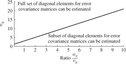
On the other hand, the relationship of the extended covariance matrix of the variable sets y0 and x0 may be described as follows
The rank of the above matrix is equal to nx, which results from the fact that
6.126 ![]()
where ![]() . Consequently, the eigendecomposition of
. Consequently, the eigendecomposition of ![]() yields a total of nx nonzero eigenvalues and the associated nx eigenvectors that span the same column space as
yields a total of nx nonzero eigenvalues and the associated nx eigenvectors that span the same column space as ![]() . Equation (6.121) defines the orthogonal complement of the estimated model subspace. A correct estimate of
. Equation (6.121) defines the orthogonal complement of the estimated model subspace. A correct estimate of ![]() and
and ![]() satisfies the constraint in (6.124) and yields ny zero eigenvalues for
satisfies the constraint in (6.124) and yields ny zero eigenvalues for ![]() .
.
6.127 ![]()
The column space of P defines the model subspace, whilst the column space of Pd defines the complementary residual subspace. The orthogonal complement to the model subspace Ξ is consequently given by
6.128 ![]()
In analogy to MLPCA and for conveniently presenting the determination of the residuals, the application of this orthogonal complement yields the following linear combinations of the error vector ![]()
which has the following error covariance matrix
Given that the two error vectors are statistically independent, that is, ![]() , (6.129) and (6.130) can be reformulated as follows
, (6.129) and (6.130) can be reformulated as follows
where ![]() and
and ![]() . Applying the block matrices
. Applying the block matrices ![]() and
and ![]() , the scaled residuals for the input and output variables are then
, the scaled residuals for the input and output variables are then
6.132 ![]()
It follows from the assumption of statistical independence between the error vectors that the covariance matrices of e and f are
The utilization of (6.131) and (6.133) now allows determining the value of the maximum likelihood objective function of (6.45)
6.134 
Including the constraint in (6.124) and a second constraint based on the last ny eigenvalues of ![]() , the objective function for estimating
, the objective function for estimating ![]() and
and ![]() becomes
becomes

Note that the above MLPLS objective function relies on estimates of ![]() ,
, ![]() and
and ![]() and is similar to that of (6.49). The steps of the iterative MLPLS algorithms that rely on the developed equations above are now listed below.
and is similar to that of (6.49). The steps of the iterative MLPLS algorithms that rely on the developed equations above are now listed below.
It is interesting to compare the MLPLS with the MLPCA algorithm, discussed in Subsection 6.1.4. The main differences between both algorithms are:
- the MLPLS algorithm does not require the computation of a Cholesky decomposition of the diagonal matrix
 , which is of dimension nx + ny;
 - the MLPLS algorithm relies on the inverse of the symmetric positive definite matrix
 of dimension nx;
 - the MLPCA algorithm requires the inverse of a diagonal matrix Li of dimension nx + ny;
- the MLPCA and MLPLS algorithms require a subsequent application of the constrained NIPALS or PLS algorithms, respectively, in order to compute the sets of latent variables;
- the MLPLS algorithm produces an EIV estimate of the regression matrix
 together with estimates of the error covariance matrices
  and
and  ; and
; and - the MLPCA algorithm produces an estimate of the PCA model subspace and an estimate of the error covariance matrix
 .
.
6.2.6 Application to a distillation process—revisited
This subsection applies the MLPLS algorithm to determine an EIV model for the reference data of the distillation process. The MRPLS model, estimated in Section 5.2, relied on the data structure in 2.51 that did not include an error term for the input variables. Selecting the parameters for the MLPLS objective function in (6.135), a1, a2 and a3, to be 0.05, 50 and 100, respectively, (6.136a) shows the estimate error variances of the input variables and (6.136b) gives estimates of the error variance of the five output variables.
6.136a 
6.136b 
Comparing the error variance for y0 obtained by the PLS/MRPLS model in Table 5.3 with the EIV estimate in (6.136b), the inclusion of ![]() for x0 gives rise to a more accurate prediction of the output variables. Moreover, the estimated error variances of the input variables as well as output variables y1, y4 and y5 are around 0.05 to 0.1 with the exception of x2 and x3 (column overhead pressure and tray 2 temperature), which have slightly smaller error variances. In contrast the error variance of the y2 and y3 concentration is significant, particularly the C5 in C4 one.
for x0 gives rise to a more accurate prediction of the output variables. Moreover, the estimated error variances of the input variables as well as output variables y1, y4 and y5 are around 0.05 to 0.1 with the exception of x2 and x3 (column overhead pressure and tray 2 temperature), which have slightly smaller error variances. In contrast the error variance of the y2 and y3 concentration is significant, particularly the C5 in C4 one.
Removing the impact of the error terms from the covariance matrices now allows estimating the LV sets. Equations (6.137) and (6.138) show the estimated r-weight and q-loading matrices. In a similar fashion to the MRPLS estimates for the r-weight matrix in 5.6, the EIV estimate outlines that the temperature of the fresh feed and the reboiler temperature do not significantly contribute to the computation of the four t-score variables. Moreover, the dominant contributions for computing each of the individual score variables are:
- the fresh feed level for the first t-score variable;
- temperature readings of tray 31 and 2 for the second t-score variable;
- tray 14 temperature and the fresh feed level for the third t-score variable; and
- the reboiler steam flow, the tray 31 and the fresh feed level for the fourth t-score variable.
In (6.137), these and other more minor contributing variables to each of the t-score variables are marked in bold.
From the parameters of the q-loading matrix, the individual t-score variables contribute to the prediction of the output variables as follows:
- t-score variable 1 has the most significant contribution to the flow rates of both output streams and to a lesser extend the C3 in C4 concentration in the top draw;
- the most dominant contribution of the second and third t-score variable is to the prediction of the C4 in C5 and the C3 in C4 concentrations; and
- t-score variable 4 is a dominant contributor of the C5 in C4 concentration.
The next questions relate to the selection of the number of source signals that the input and output variables commonly share and what the contribution of each set of latent variables explains to the covariance and cross-covariance matrices. An answer to both of these questions lies in evaluating 2.102 to 2.104. Figure 6.17 plots the ratios produced by these equations for k = 1 … 8 for the maximum likelihood and the standard MRPLS algorithms. It is important to note that the maximum likelihood MRPLS algorithm relies on covariance matrices for which the variance of each error term is subtracted from the estimated covariance matrices.
Figure 6.17 Deflation of ![]() ,
, ![]() and
and ![]() using extracted latent variable sets (left plot → MRPLS model; right plot → maximum likelihood MRPLS model).
using extracted latent variable sets (left plot → MRPLS model; right plot → maximum likelihood MRPLS model).
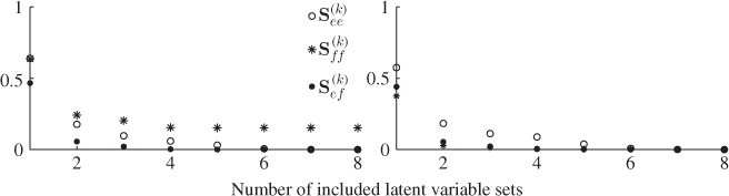
This is different for the original MRPLS algorithm, which relies on the estimated covariance and cross-covariance matrices. It is also important to note that the deflation of the covariance matrices is not required for the computationally efficient MRPLS algorithm in Table 10.3. However, in order to compute the contribution of each set of latent variables from these matrices, a deflation procedure after the model building phase was carried out.
Addressing the first question, both plots in Figure 6.17 confirm that subtracting the contribution of the first four t-score variables maximally exhausted the squared sum of the elements of the cross-covariance matrix. For the maximum likelihood MRPLS model, the squared sum of the elements of this matrix are very close to zero, implying that there is no common cause variation left between both variable sets that requires the inclusion of a fifth source variable. The selection of n = 4 is therefore confirmed.
Different to its maximum likelihood counterpart, there is a remaining value of about 0.15 for the covariance matrix ![]() .8 This is not surprising, given that the error variables are assumed to be uncorrelated to the input variables. The decrease in the squared sum of the covariance matrix
.8 This is not surprising, given that the error variables are assumed to be uncorrelated to the input variables. The decrease in the squared sum of the covariance matrix ![]() is similar for both models. That these values are slightly smaller for the maximum likelihood MRPLS algorithm is, again, a result of excluding the estimated variance of the error terms.
is similar for both models. That these values are slightly smaller for the maximum likelihood MRPLS algorithm is, again, a result of excluding the estimated variance of the error terms.
Finally, the regression model obtained by the maximum likelihood MRPLS algorithm for n = 4 can be compared to that computed by the MRPLS one in Table 5.4. Significant differences between both regression matrices are that the maximum likelihood MRPLS regression model confirms:
- that column pressure x2, tray 2 temperature x3 and fresh feed temperature x4 have the most significant impact on the C4 in C5 concentration y5;
- that the reboiler stream flow x5 is mostly affecting the impurities y2 and y3;
- that the flow rate of the fresh feed x7 impacts not only the flow rate of the output stream but also C3 in C4 and the C5 in C4 concentrations; and
- that the reboiler temperature mainly affects the C5 in C4 concentration y3.
Both regression matrices, however, suggest that the tray 31 temperature x6 has an affect on the concentrations of the top and bottom draw.
The information that can be extracted from the EIV estimate of the regression matrix describes the underlying causal relationships between the input and output variables correctly. It is important to recall that the static MRPLS model does not represent a causal dynamic mechanistic model that describes the physical and chemical relationships between the process variables. However, the steady state relationships that can be extracted from the regression matrix in Table 6.14 describe a correct relationship between the input and output variables.
Table 6.14 Coefficients of regression model for n = 4.
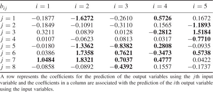
6.3 Robust model estimation
Besides process monitoring, all branches of data chemometrics and analytical chemistry, for example, in industrial and academic research deal with large amounts of data, which can be subjected to errors, including bias, for example resulting from the poor calibration of measurement devices, and sporadic outliers, that can arise for any number of reasons. The first type is usually related to small persistent residual parts (offset) during the measurements being taken, whilst the second one is associated with large residuals and most of the time affect only single observations.
Detecting a bias is straightforward by carefully inspecting the recorded data and applying a priori knowledge and experience. The same cannot be said for outliers, as they infrequently arise, may easily be overlooked in large data sets and can have a profound and undesired impact upon the accuracy of the estimated parameters, for example the estimation of the data covariance matrix or the control limits for univariate monitoring statistics. In general, outliers can be divided into three categories (Møller et al. 2005):
Figure 6.18 gives a graphical account of each type of outlier for three process variables that can be described, according to 2.2, by two source signals and a superimposed error vector. Whilst the normal or ‘sound’ samples locate in the vicinity of the model subspace, the outliers have large departures either from the model subspace (large residuals g1 and g2 for the first and second outliers) and/or the cluster of normal samples. A robust estimation of parameters entails the removal or reduction of the impact of outliers upon the estimation and the aim of this section is to summarize research work, including recent trends, reported in the literature.
Figure 6.18 Illustration of the three different types of outliers in a data space.
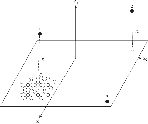
It should be noted that outliers in recorded reference data are identifiable using the covariance matrix ![]() and the error covariance matrix
and the error covariance matrix ![]() if known a priori. As Figure 6.18 illustrates that outliers 1 and 2 possess a large residual part by definition, whilst outliers 2 and 3 are associated with a large variance part. In case the covariance matrices are available it is sufficient to evaluate a statistical test over the reference samples to determine whether a particular sample is an outlier or not. However, these matrices, particularly the error covariance matrix, are usually unknown and need to be estimated from the reference set. Over the past few decades, a plethora of methods have been proposed to produce robust estimates for parameters, such as variable mean and covariance matrix.
if known a priori. As Figure 6.18 illustrates that outliers 1 and 2 possess a large residual part by definition, whilst outliers 2 and 3 are associated with a large variance part. In case the covariance matrices are available it is sufficient to evaluate a statistical test over the reference samples to determine whether a particular sample is an outlier or not. However, these matrices, particularly the error covariance matrix, are usually unknown and need to be estimated from the reference set. Over the past few decades, a plethora of methods have been proposed to produce robust estimates for parameters, such as variable mean and covariance matrix.
The discussion of robust methods can be roughly classified into two categories:
- accept all the data points and try to find a robust estimator which reduces the impact of outliers; and
- maintain the traditional estimators and try to eliminate the outliers (trimming) before the estimation by using some cluster property.
The literature regards the first approach as robust regression or robust parameter estimation, whilst the second one can be categorized as the trimming approach. The next two subsections summarize associated methods for both of these approaches. The aim of this subsection is to give a brief overview of existing methods. A more detailed and specific treatment of this topic is available in references Daszykowski (2007); Liang and Kvalheim (1996) and Møller et al. (2005) for example.
6.3.1 Robust parameter estimation
Robust regression methods can be further divided into (i) robust estimates of the moments, (ii) projection pursuit, (iii) M estimators and (iv) least median of squares.
6.3.1.1 Robust estimation of the moments
The definition of processes the produce variables that follow a Gaussian distribution require the estimation of the data location (mean vector) and spread (covariance matrix). The mean vector can be viewed as a least squares estimator
6.139 
which includes squared summation elements and is, accordingly, sensitive to the presence of outliers. A robust alternative is the use of the median of the samples
6.140 
or the Stahel-Donoho location estimator (Donoho 1982; Stahel 1981)
where dk = d(r(z(k), Z)) is a weighting function, such as the iteratively re-weighted least squares function (Phillips and Eyring 1983), and r(z(k), Z) is defined as follows
Here, ![]() and
and ![]() are the median and the median absolute deviation of the projections of the samples stored in Z onto
are the median and the median absolute deviation of the projections of the samples stored in Z onto ![]() , respectively, and | · | is the absolute value. For PLS, Kruger et al. (2008a,b,c) proposed an iterative algorithm on the basis of (6.142) to discriminate outliers from sound observation.
, respectively, and | · | is the absolute value. For PLS, Kruger et al. (2008a,b,c) proposed an iterative algorithm on the basis of (6.142) to discriminate outliers from sound observation.
The variance, or the second order moments of a variable, is also calculated as the sum of squares, and therefore affected by outliers. The literature proposed a number of methods for providing a robust estimation of variance, where the median absolute deviation (MAD) and the more efficient Sn and Qn estimators are among the most popular ones (Hampel 1974; Rousseeuw and Croux 1993)
with b = 1.4826, c = 1.1926, d = 2.219 and med abbreviates median. A detailed discussion of these estimators is given in Rousseeuw and Croux (1993). With the availability of robust estimates for mean and variance, a robust pretreatment such as of the recorded data, such as mean centering and scaling, can be carried out. A direct estimation of the covariance matrix can be determined as the Stahel-Donoho scale estimator
6.144 
The mean vector can be obtained using (6.141).
6.3.1.2 Projection pursuit
The projection pursuit approach substitutes a traditional objective function by a robust one (Daszykowski 2007). In the case of PCA, Section 2.1 pointed out that the associated objective function involves the maximization of the variance of the ith score variable, ti. Equation (6.143) summarizes robust estimates for the variable variance and the projection pursuit can be seen as a simple regression-based approach to obtain a robust objective function, for example
6.145 ![]()
Here, PI stands for projection index and represents the robust objective functions. As examples, various objective functions for the data mean ![]() are summarized in (6.143).
are summarized in (6.143).
6.3.1.3 M-estimator
This is a maximum likelihood estimator for minimizing the residuals, for example the residuals associated with the jth process variable of a PCA model gj(k)
6.146 
for which a variety of estimators have been proposed, including
6.147 
The parameter θ serves as a tuning parameter.
6.3.1.4 Least median of squares—LMS
This is one of the most popular methods and was developed by Rousseeuw (1984) for robustly estimating variance. This technique replaces the sum of the squared residuals with the robust median
6.148 ![]()
In other words, the estimator is the smallest value for the median of the squared residuals computed over the complete reference data set. In contrast to the M-estimator, the LMS estimator does not present a weighted least squares problem and the determination of a solution can be computationally demanding.
6.3.2 Trimming approaches
Trimming approaches exclude some extreme samples that are considered outliers for determining a robust estimate. Associated methods that the research literature has proposed include the trimmed least squares, multivariate trimming, the minimum volume estimator and the minimum covariance determinant estimator.
6.3.2.1 Least trimmed squares—LTS
This is the simplest approach and relates to the classification of samples based on their residue magnitude (Rousseeuw 1984). Those samples producing the largest residuals are considered outliers and, accordingly, excluded from the computation of the estimate. The LTS method gives rise to the solution of the following minimization problem
6.149 
where ![]() is referred to as an ordered residual that is ranked according to the magnitude of the residual (crescent magnitude). Those with the largest magnitude are removed so that K− ≤ K samples remain. With regards to Figure 6.18, it should be noted that the LTS method only tackles samples that produce orthogonal or bad leverage outliers.
is referred to as an ordered residual that is ranked according to the magnitude of the residual (crescent magnitude). Those with the largest magnitude are removed so that K− ≤ K samples remain. With regards to Figure 6.18, it should be noted that the LTS method only tackles samples that produce orthogonal or bad leverage outliers.
6.3.2.2 Multivariate trimming—MVT
Instead of the use of residuals, the MVT technique relies on the distance between the data points to produce a robust estimate (Gnanadesikan and Kettenring 1972; Maronna 1976). Assuming the data follow a Gaussian distribution function, the MVT method iteratively discards extreme values which, in turn, generates a PDF that shows significant departures from the theoretical one.
6.3.2.3 Minimum volume estimator—MVE
This approach is similar to the MVT technique in that it assumes that the data can be described by a predefined shape. More precisely, the MVE method determines a multivariate ellipsoid that hugs at least 50% of the samples. Points that fall outside this ellipsoid are not considered for estimating a model.
6.3.2.4 Minimum covariance determinant estimator—MCD
The MCD method is similar in approach to the MVE and MVT techniques in that it relates to the assumed cluster property of uncorrupted observations (Gnanadesikan and Kettenring 1972; Maronna 1976). Utilizing a cross-validation procedure, this technique is able to give a robust estimation of the data location and dispersion. In a univariate case, the MCD approach reduces to a LTS estimator where each data point receives a weight of one if it belongs to the robust confidence interval and zero otherwise. Rocke and Woodruff (1996); Rousseeuw and Driessen (1999) pointed out that MCD is theoretically superior to MVT, and Davies (1992) showed that MCD possesses better statistical properties compared to MVE.
6.4 Small sample sets
Reference data that include relatively few samples compared to the number of process variables present challenges in determining confidence limits/regions for statistical inference. Numerous textbooks on statistics outline that the confidence limits, determining the acceptance region for estimating parameters or hypothesis tests, widens with a reduction in the size of the reference set. This, in turn, can have a profound and undesirable effect upon the number of Type I and II errors.
As an example, the confidence interval for estimating the variable mean for a particular process variable z is given by
6.150 ![]()
The true mean value, ![]() lies under the assumption that E{(z −
lies under the assumption that E{(z − ![]() )2} = σ2 is known within this confidence interval, limited by the parameter a
)2} = σ2 is known within this confidence interval, limited by the parameter a![]() , which is given by
, which is given by
Here, c defines the confidence interval for a zero mean Gaussian distribution of unit variance, ϕ( · ), and is given by ![]() . For example, significances of 0.05 and 0.01 require c to be 1.960 and 2.576, respectively. The relationship in (6.151), however, shows a direct dependence between the length of the confidence interval for estimating
. For example, significances of 0.05 and 0.01 require c to be 1.960 and 2.576, respectively. The relationship in (6.151), however, shows a direct dependence between the length of the confidence interval for estimating ![]() and the number of samples, K, since σ and c are constant. Qualitatively, if K is large a
and the number of samples, K, since σ and c are constant. Qualitatively, if K is large a![]() will be small and vice versa.
will be small and vice versa.
The same problem emerges when determining the upper and lower control limits for Shewhart charts, and the control limits for the Hotelling's T2 and Q statistics. This section revisits the issue of constructing non-negative quadratic forms and associated control limits using small reference sets. A non-negative quadratic form, such as the Hotelling's T2 statistic, has the following definition
6.152 ![]()
Here,
 and
and  are a data vector and the estimated sample mean, respectively; and
 is the estimate of
  for a total of K independent samples.
The estimation of the data covariance matrix ![]() follows a Wishart distribution (Tracey et al. 1992). Under the assumption that the estimation of
follows a Wishart distribution (Tracey et al. 1992). Under the assumption that the estimation of ![]() is independent of each z(k), k = {1, 2, … , K}, the T2 statistic follows an F-distribution
is independent of each z(k), k = {1, 2, … , K}, the T2 statistic follows an F-distribution
6.153 ![]()
Here, the estimates of ![]() and
and ![]() have the distributions
have the distributions
 ; and
; and ,
,
where ![]() (.) is a Wishart distribution. The often observed high degree of correlation in the recorded variable set, described in Section 1.2 and Chapter 2, is addressed by defining a reduced set of LVs
(.) is a Wishart distribution. The often observed high degree of correlation in the recorded variable set, described in Section 1.2 and Chapter 2, is addressed by defining a reduced set of LVs
6.154 ![]()
Chapter 3 showed that n < nz yields two non-negative quadratic forms for PCA, and n < nx gives rise to three non-negative quadratic forms for PLS. Concentrating on PCA, the Hotelling's T2 and Q statistics are defined as
6.155 ![]()
and
6.156 ![]()
respectively. As before, ![]() and
and ![]() store estimated dominant n eigenvectors and eigenvalues of
store estimated dominant n eigenvectors and eigenvalues of ![]() , respectively.
, respectively.
The above remark relates to the estimation of Λ
6.157 
which follows a Wishart distribution if and only if ![]() follow a multivariate Gaussian distribution and
follow a multivariate Gaussian distribution and ![]() is estimated from a different sample set. If this assumption is not met, the Hotelling's T2 statistic does not follow an F-distribution. Approximations of the Q statistic have been proposed in Nomikos and MacGregor (1995).
is estimated from a different sample set. If this assumption is not met, the Hotelling's T2 statistic does not follow an F-distribution. Approximations of the Q statistic have been proposed in Nomikos and MacGregor (1995).
The following Monte Carlo experiment illustrates the problem of determining the control limits for non-negative quadratic forms if K is small. This example is similar to that in Ramaker et al. (2004) and includes fifteen process variables, three source variables and an error vector
where ![]() ,
, ![]() , and
, and ![]() are arbitrary unit length vectors and s1(k), s2(k) and
are arbitrary unit length vectors and s1(k), s2(k) and ![]() are statistically independent Gaussian sequences of zero mean and variances 5, 3 and 1, respectively. The error vector
are statistically independent Gaussian sequences of zero mean and variances 5, 3 and 1, respectively. The error vector ![]() .
.
From this process, a number of reference sets was simulated, which form the the basis for determining the Hotelling's T2 and Q statistics. To determine the Type I error for a significance of α, one additional set of 250 test samples that was not used as a reference set were simulated. The reference sets included K = 20, 50, 100, 500 and 1000 samples and were simulated a total of 100 times (Monte Carlo experiment). The control limits were obtained for each experiment with a significance of α = 0.05. Figure 6.19 shows the results of these Monte Carlo experiments for a variety of retained components, ranging from 1 to 14.
Figure 6.19 Type I error [%] for α = 0.05.
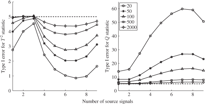
Given that each point in Figure 6.19 represents the average Type I error, it is interesting to note that the smallest departure of the T2 statistic arises for n = 3. Any other n produced a more significant departure. As expected, the smaller the size of the reference set, the more pronounced the departure from the theoretical 5%. Whilst this example yielded an up to 4% difference in Type I error for the T2 statistic and K = 20, a more considerable impact is noticeable for the Q statistic.
To overcome this issue, Ramaker et al. (2004) proposed the use of leave-one-out cross validation (LOO CV)9 to determine the score variables and the mismatch between the original variable, z0, and its projection onto the model subspace ![]() . More precisely, the kth data sample is removed from the reference set and the remaining K − 1 samples are used to estimate P−k. This is followed by a determination of the retained scores and the residual vector for the kth sample, that is
. More precisely, the kth data sample is removed from the reference set and the remaining K − 1 samples are used to estimate P−k. This is followed by a determination of the retained scores and the residual vector for the kth sample, that is ![]() and
and ![]() .
.
The application of LOO CV therefore produces a total of K t-scores and residual vectors which are then used to determine the covariance matrix ![]() and the control limit for the Q statistic. Comparing Figures 6.19 and 6.20 allows a direct comparison between the original approach and LOO CV, respectively. Although the latter technique yielded a significant reduction in the Type I error of the Q statistic, it did not show any improvement for the Hotelling's T2 statistic. To the contrary, the LOO CV approach produced a very significant increase in the Type I errors.
and the control limit for the Q statistic. Comparing Figures 6.19 and 6.20 allows a direct comparison between the original approach and LOO CV, respectively. Although the latter technique yielded a significant reduction in the Type I error of the Q statistic, it did not show any improvement for the Hotelling's T2 statistic. To the contrary, the LOO CV approach produced a very significant increase in the Type I errors.
Figure 6.20 Type I error [%] (LOO CV) for α = 0.05.
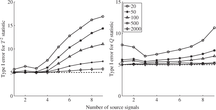
Although the work in Ramaker et al. (2004) highlighted that non-negative squared forms are difficult to establish using small reference sets, it did not identify a theoretical rationale that explains the unwanted increase in number of Type I error (Q statistic) and Type II error (Hotelling's T2 statistic). Analyzing Remark 6.4.1, however, reveals that the Hotelling's T2 statistic can only follow an F-distribution when the estimate of Stt relies on data that were not used for the estimation of P. For conventional PCA, however, ![]() and
and ![]() store the eigenvectors and the eigenvalues of
store the eigenvectors and the eigenvalues of ![]() and hence, statistical independence is not guaranteed.
and hence, statistical independence is not guaranteed.
Moreover, the use of LOO CV produces a total of K different model subspaces and residual subspaces. This, in turn, implies that there is no guarantee that the estimate of Stt follows a Wishart distribution. Despite the fact that this approach produced a substantial reduction in Type I error for the Q statistic, the sequence of K residual vectors corresponds, therefore, to a total of K different residual subspaces. A more minor issue is the computational demand to implement the LOO CV approach.
Next, we discuss an alternative approach that overcomes the problems of the LOO CV technique. To improve this method, a more rigorous separation of the data is required to guarantee statistical independence for distribution functions of:
 and z0 (to estimate Stt and
  ); and
- g and (to estimate Qα).
The proposed division produces two independent reference sets
6.159 ![]()
and
6.160 ![]()
of equal length. Next, an estimate of P, ![]() , based on
, based on
6.161 
is obtained, followed by computing
6.162 
The proposed division of the reference data set guarantees that the distribution functions for ![]() and Z2 are statistically independent. This, in turn, implies that
and Z2 are statistically independent. This, in turn, implies that
6.163 ![]()
and
6.164 ![]()
Moreover, using this data separation, the score variables now have the following distribution for new observations that are not included in Z1 and Z2
6.165 ![]()
and consequently, the T2 statistic follows an F-distribution, that is
6.166 
Utilizing the same approach to determine the ![]() statistic, that is, computing the residual vectors from the reference set Z2 and the estimate of P from Z1, Figure 6.21 shows, as expected, that the 50% percentile of the Monte Carlo experiments for α = 0.05. Note that an equal separation of the reference data set resulted in the determination of only 10 PCs if 20 samples were available. This, on the other hand, implied that a total of nine discarded PCs could be analyzed. For small sample sets, including less than 100 samples, an increase in the Type I error for the Q statistic arose. This can be attributed to the fact that the distribution function of the Q statistic, used to determine
statistic, that is, computing the residual vectors from the reference set Z2 and the estimate of P from Z1, Figure 6.21 shows, as expected, that the 50% percentile of the Monte Carlo experiments for α = 0.05. Note that an equal separation of the reference data set resulted in the determination of only 10 PCs if 20 samples were available. This, on the other hand, implied that a total of nine discarded PCs could be analyzed. For small sample sets, including less than 100 samples, an increase in the Type I error for the Q statistic arose. This can be attributed to the fact that the distribution function of the Q statistic, used to determine ![]() , is an approximation, which requires a larger data set to be accurate.
, is an approximation, which requires a larger data set to be accurate.
Figure 6.21 Number of Type I error [%] (two-stage PCA) for a significance of 0.05.
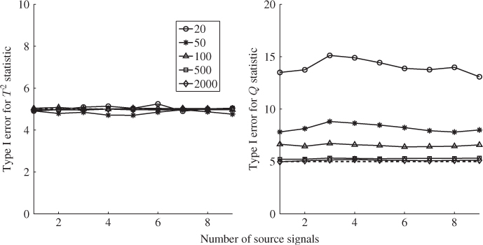
The main focus of this section, however, is on the T2 statistic, which the data division showed to outperform the approach by Ramaker et al. (2004). More precisely, the 50% percentile is very close to α = 0.05 for any combination of the number of retained PCs and size of the reference sets.
6.5 Tutorial session
Question 1
Explain why PCA produces a biased estimation of the orientation of the model and residual subspaces when the error covariance matrix for a set of process variables, z0, is not of the form ![]() . What is the impact of a biased estimation in terms of extracting the source and error variables?
. What is the impact of a biased estimation in terms of extracting the source and error variables?
Question 2
For the application of maximum likelihood PCA, What is the reason for constraining the maximum number of estimated parameters according to (6.46)? In case the number of error variances is larger than this maximum number, discuss ways to estimate the error covariance matrix.
Question 3
Discuss the advantage of using PLS over standard ordinary least squares in determining a parametric regression model if the input variable set is highly correlated. What happens if there is a linear dependency among the input variable set?
Question 4
Explain why OLS, PLS and MRPLS produce a biased estimation of the parameter regression matrix between the input and output variables if both variable sets are corrupted by an error term. Explain the impact of this estimation bias upon the extraction of source signals according to the PLS and MRPLS data structures in 2.24 and 2.51?
Question 5
What are outliers and how can they be categorized? What is the effect of outliers on the determination of PCA and PLS models?
Project 1
Based on a Monte Carlo simulation, use the example described in (6.53) to (6.55) and alter the magnitude of the individual diagonal elements of Sgg as well as their differences in value and compare the accuracy of the model subspace between the MLPCA and the PCA estimates. How does increasing or reducing the number of samples affect the accuracy?
Project 2
Contrast the stopping rule introduced in Subsection 6.1.6 with those discussed in Subsection 2.4.1 using the simulation example in (6.53) to (6.55). For this comparison, change the magnitude of the individual diagonal elements of Sgg as well as their differences in value. How does increasing or reducing the number of samples affect the estimate of n?
Project 3
Repeat the Monte Carlo experiment for the data structure described in (6.87) to (6.89c). Comment on the experimental results in terms of the accuracy of the OLS estimation for a varying sample size K = 100, 200, 500, 1000 and 2000. Compare the results with the PLS estimation of the regression matrix for each K by varying the number of retained LV sets ![]() , 2, … , 10 and comment on the results obtained. Is there an optimal trade off between the accuracy of the parameter estimation, model prediction error and the number of retained sets of LVs for each K?
, 2, … , 10 and comment on the results obtained. Is there an optimal trade off between the accuracy of the parameter estimation, model prediction error and the number of retained sets of LVs for each K?
Project 4
For PCA, study the impact of outliers model using a Monte Carlo simulation on the basis of the example described in (6.53) to (6.54) by defining ![]() , with
, with ![]() . Inject 1%, 2%, 5%, 10%, 20% and 50% of outliers into a simulated reference set of K = 200, 500, 1000, 2000 and 5000 samples and comment upon the accuracy of the estimated model and residual subspaces. Next, use the Stahel-Donoho scale estimator to determine a robust estimation of the data covariance matrix and examine how the accuracy of estimating the model and residual subspaces improves when using the robust estimate?
. Inject 1%, 2%, 5%, 10%, 20% and 50% of outliers into a simulated reference set of K = 200, 500, 1000, 2000 and 5000 samples and comment upon the accuracy of the estimated model and residual subspaces. Next, use the Stahel-Donoho scale estimator to determine a robust estimation of the data covariance matrix and examine how the accuracy of estimating the model and residual subspaces improves when using the robust estimate?
Project 5
Repeat the Monte Carlo simulation described in (6.158) by altering the error variance ![]() , the variances of the source signals
, the variances of the source signals ![]() ,
, ![]() and
and ![]() and the number of retained LV sets.
and the number of retained LV sets.
1 It is assumed that the absolute elements of ![]() are bounded and hence J( · ) > 0.
are bounded and hence J( · ) > 0.
2 It is assumed here that Ξ1 has full rank n.
3 The value of 10−12 is a possible suggestion; practically, smaller thresholds can be selected without a significant loss of accuracy.
4 The value of 10−12 is a possible suggestion; practically, smaller thresholds can be selected without a substantial loss of accuracy.
5 The generalized inverse of a matrix is often referred to as the Moore-Penrose pseudo inverse.
6 Assumed here to be 0.7714, whilst the true ![]() is 0.779 according to (6.89c).
is 0.779 according to (6.89c).
7 The value of 10−12 is a possible suggestion; practically, smaller thresholds can be selected without a substantial loss of accuracy.
8 After deflating the four sets of latent variables computed by the MRPLS algorithm.
9 The principle of which is discussed in Subsection 2.4.1.