
11
Bayesian Estimation
In several applications there is enough (statistical) information on the most likely values of the parameters θ to be estimated even before making any experiment, or before any data collection. The information is encoded in terms of the a‐priori pdf p(θ) that accounts for the properties of θ before any observation (Chapter 6). Bayesian methods make efficient use of the a‐priori pdf to yield the best estimate given both the observation x and the a‐priori knowledge on the admissible values from p(θ).
Recall that MLE is based on the conditional pdf ![]() that sets the probability of the specific observation xk for any choice
that sets the probability of the specific observation xk for any choice ![]() , but these choices are not all equally likely. In the Bayesian approach, the outcome of the k th experiment is part of a set of (real or conceptual) experiments with two random sets θ and x, that in the case of an additive noise model
, but these choices are not all equally likely. In the Bayesian approach, the outcome of the k th experiment is part of a set of (real or conceptual) experiments with two random sets θ and x, that in the case of an additive noise model ![]() are θ and w. The joint pdf is
are θ and w. The joint pdf is
but it is meaningful to consider for each experiment (or realization of the rv x) the pdf of the parameter θ conditioned to the k th observation ![]() (here deterministic) according to Bayes’ rule, which gets the pdf of the unobserved θ
(here deterministic) according to Bayes’ rule, which gets the pdf of the unobserved θ

with γ as a scale factor to normalize the pdf. The a‐posteriori pdf ![]() is the pdf of the unknown parameter θ after the observation
is the pdf of the unknown parameter θ after the observation ![]() , and reflects the statistical properties of θ after the specific experiment.
, and reflects the statistical properties of θ after the specific experiment.
To further stress the role of the a‐priori pdf in Bayesian methods, we can make reference to Figure 11.1 to derive the a‐posteriori pdf ![]() (as routinely employed in the notation, the specific observation
(as routinely employed in the notation, the specific observation ![]() is understood), which is obtained by multiplying the a‐priori p(θ) and the conditional pdf
is understood), which is obtained by multiplying the a‐priori p(θ) and the conditional pdf ![]() . In Figure 11.1, θ is scalar (number of parameters
. In Figure 11.1, θ is scalar (number of parameters ![]() ) and the a‐priori pdf shows some values that are more or less likely than others. After the observation, the conditional pdf
) and the a‐priori pdf shows some values that are more or less likely than others. After the observation, the conditional pdf ![]() is the one that is used in the ML method and it has a different behavior from the a‐priori one. More specifically, the maximum of the conditional pdf provides the MLE θML without any knowledge of the probability of the values of θ. After multiplying the conditional pdf with the a‐priori pdf, the a‐posteriori pdf
is the one that is used in the ML method and it has a different behavior from the a‐priori one. More specifically, the maximum of the conditional pdf provides the MLE θML without any knowledge of the probability of the values of θ. After multiplying the conditional pdf with the a‐priori pdf, the a‐posteriori pdf ![]() compounds the likelihood of the parameters regardless of the knowledge of their probability, and the probability associated to each value of the parameters, by the a‐priori pdf p(θ).
compounds the likelihood of the parameters regardless of the knowledge of their probability, and the probability associated to each value of the parameters, by the a‐priori pdf p(θ).
Figure 11.1 Bayesian estimation ( ).
).
Based on the a‐posteriori pdf, Bayesian estimation can follow two different strategies:
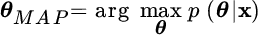
- Maximum a‐posteriori (MAP) estimation: the estimate is the value that maximizes the a‐posteriori probability
- Minimum mean square error (MMSE) estimation: the estimate can be in the baricentral position wrt the a‐posteriori pdf:
This is the mean value of the conditional pdf
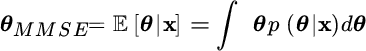
 , and it is commonly referred to as the MMSE estimate as clarified below.
Any estimator ![]() depends on the observations, but under the Bayesian assumptions, the error
depends on the observations, but under the Bayesian assumptions, the error ![]() is an rv that depends on both the data x and the rv θ with pdf p(θ). The corresponding Bayesian MSE (Section 6.3.2):
is an rv that depends on both the data x and the rv θ with pdf p(θ). The corresponding Bayesian MSE (Section 6.3.2):

is evaluated wrt the randomness of the data and θ. The MSE is thus the “mean” in the sense that it accounts for all possible choices of the rv θ weighted by the corresponding occurrence probability p(θ) as ![]() . The minimization of the MSE seeks for the parameter value that minimizes the
. The minimization of the MSE seeks for the parameter value that minimizes the ![]() as a function of
as a function of ![]() . From
. From

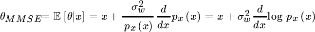
since p(x) is semipositive definite and independent of ![]() , it is enough to minimize the term within the bracket (i.e., the MSE conditioned to a specific observation x) by nulling the gradient:
, it is enough to minimize the term within the bracket (i.e., the MSE conditioned to a specific observation x) by nulling the gradient:

Rearranging terms yields the MMSE estimator

as the estimator that minimizes the MSE for all possible (and random) outcomes of the parameters θ.
Remark: The illustrative example at hand helps to raise some issues based on which Bayesian estimators have to be preferred. There is no unique answer, but it depends on the application. The example shows a multimodal a‐posteriori pdf and MAP selects one value that occurs with the greatest probability. On the other hand, the MAP choice could experience large errors In the case that some outcomes are in other modes of the pdf. The MMSE is the best “mean solution” that could coincide with a value that is unlikely, if not admissible (e.g., ![]() ). In general, for multimodal a‐posteriori pdf, the maximum (MAP) and the mean (MMSE) of the a‐posteriori pdf do not coincide, and choosing one or another depends on the specific application problem. Some care should be taken to avoid the Buridan’s ass paradox1 and estimate a value that is a nonsense for the problem at hand, but still compliant with the estimator’s metric—as for the MMSE estimate for binary valued parameters (Section 11.1.3). On the other hand, if the a‐posteriori pdf is unimodal and even, both MAP and MMSE coincide, as in the case of Gaussian rvs—a special and favorable case as detailed below.
). In general, for multimodal a‐posteriori pdf, the maximum (MAP) and the mean (MMSE) of the a‐posteriori pdf do not coincide, and choosing one or another depends on the specific application problem. Some care should be taken to avoid the Buridan’s ass paradox1 and estimate a value that is a nonsense for the problem at hand, but still compliant with the estimator’s metric—as for the MMSE estimate for binary valued parameters (Section 11.1.3). On the other hand, if the a‐posteriori pdf is unimodal and even, both MAP and MMSE coincide, as in the case of Gaussian rvs—a special and favorable case as detailed below.
11.1 Additive Linear Model with Gaussian Noise
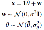
This observation is modeled by ![]() , in which the scalar parameter θ is random and should be estimated from a single observation with additive Gaussian noise:
, in which the scalar parameter θ is random and should be estimated from a single observation with additive Gaussian noise: ![]() . The Gaussian model is discussed first with
. The Gaussian model is discussed first with ![]() , and then extended to the case of non‐Gaussian rv θ. It will be shown that Bayesian estimators become non‐linear for an arbitrary pdf, and this motivates the interest in linear estimators even when non‐linear estimators should be adopted, at the price of some degree of sub‐optimality.
, and then extended to the case of non‐Gaussian rv θ. It will be shown that Bayesian estimators become non‐linear for an arbitrary pdf, and this motivates the interest in linear estimators even when non‐linear estimators should be adopted, at the price of some degree of sub‐optimality.
11.1.1 Gaussian A‐priori: 
Single Observation 
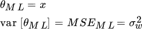
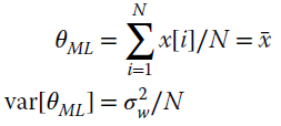
In MLE, the value of the parameter θ does not change even if considering multiple experiments. For a single observation, the MLE is
Assuming now that for each observation (composed of a single sample) the parameter value θ is different and drawn from a Gaussian distribution ![]() where
where ![]() and
and ![]() are known, the joint pdf is
are known, the joint pdf is ![]() while the pdf of θ conditioned to a specific observation (a‐posteriori pdf) is
while the pdf of θ conditioned to a specific observation (a‐posteriori pdf) is

up to a scale Γ. Rearranging the exponentials, the a‐posteriori pdf is
This shows the general property (see Section 11.2) that for additive linear models, the a‐posteriori pdf is Gaussian if all terms are Gaussian. Returning to the specific example, the terms involved are
The second term shows that the variance of the a‐posteriori pdf is always smaller than the a‐priori (![]() ) except when noise dominates the measurements (
) except when noise dominates the measurements (![]() ) and
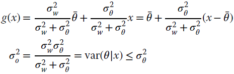
) and ![]() . The maximum of the a‐posteriori
. The maximum of the a‐posteriori ![]() when Gaussian is for
when Gaussian is for
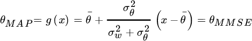
Considering the symmetry of the Gaussian pdf, it is straightforward to assert that ![]() . It is interesting to note that for
. It is interesting to note that for ![]() , the a‐priori information dominates and
, the a‐priori information dominates and ![]() regardless of the specific observation, while for
regardless of the specific observation, while for ![]() , a‐priori information becomes irrelevant (in this case the a‐priori information is diffuse or non‐informative) and
, a‐priori information becomes irrelevant (in this case the a‐priori information is diffuse or non‐informative) and ![]() as in MLE. This is another general property: when the a‐priori pdf p(θ) is uniform, there is no difference between one choice and the other, and the Bayesian estimator cannot rely on any a‐priori pdf; in this case the MAP coincides with the MLE.
as in MLE. This is another general property: when the a‐priori pdf p(θ) is uniform, there is no difference between one choice and the other, and the Bayesian estimator cannot rely on any a‐priori pdf; in this case the MAP coincides with the MLE.
The Bayesian MSE should take into account both the parameter and noise as rvs:

and ![]() for diffuse a‐priori (
for diffuse a‐priori (![]() ).
).
The Bayesian MSE can be evaluated in the following alternative way:

Note that MSEML(θo) is the MSE for deterministic ![]() as for MLE. Since for the example here
as for MLE. Since for the example here ![]() , but θMMSE optimizes the Bayesian MSE and not the MSEML(θo), the estimate θMAP cannot be optimal for the deterministic value
, but θMMSE optimizes the Bayesian MSE and not the MSEML(θo), the estimate θMAP cannot be optimal for the deterministic value ![]() (incidentally, it is biased). Nevertheless, when the MSE is evaluated by taking into account the variability of θo, the Bayesian estimation shows its superiority with respect to the ML estimation for any arbitrary (but still with pdf
(incidentally, it is biased). Nevertheless, when the MSE is evaluated by taking into account the variability of θo, the Bayesian estimation shows its superiority with respect to the ML estimation for any arbitrary (but still with pdf ![]() ) value of θ.
) value of θ.
To summarize, the Bayesian MSE of the MMSE estimator is always lower than the MSE of the MLE. This is due to fact that the MMSE estimator exploits the available a‐priori information on the parameter value.
Multiple Observations 
We can consider a more complex (but somewhat more realistic) example with N observations characterized by independent noise components with the same value of the parameter θ, that in turn it can change over the realizations. The model can be written as:

Estimation of the parameter is the sample mean (see, e.g., Section 6.7)
while the MMSE estimator is linear (it will be derived in the following section) and it is given by
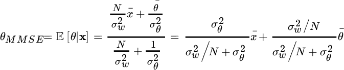
It is interesting to remark that the MMSE estimation is a linear combination between the mean parameter value ![]() (known a‐priori) and the sample mean
(known a‐priori) and the sample mean ![]() . For
. For ![]() the a‐priori information becomes irrelevant and
the a‐priori information becomes irrelevant and ![]() while for
while for ![]() we have
we have ![]() . From the symmetry of the Gaussian a‐posteriori pdf,
. From the symmetry of the Gaussian a‐posteriori pdf, ![]() .
.
11.1.2 Non‐Gaussian A‐Priori
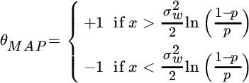
The observation ![]() is the sum of two random variables, only one of which (here noise) is Gaussian, say
is the sum of two random variables, only one of which (here noise) is Gaussian, say ![]() . The MMSE follows from the definition:
. The MMSE follows from the definition:

where the following two equalities have been used to derive the last term: ![]() and
and  . The general relationship of the MMSE estimator is2
In other words, the MMSE estimator is a non‐linear transformation of the observation x and its shape depends on the pdf of the observation ![]() . This example can be generalized: the MMSE estimator is non‐linear except in Gaussian contexts (the proof is simple: just set
. This example can be generalized: the MMSE estimator is non‐linear except in Gaussian contexts (the proof is simple: just set ![]() ; this gives
; this gives ![]() therefore, in this case, the MMSE estimator is linear and it coincides with the one reported previously in Section 11.1.1).
therefore, in this case, the MMSE estimator is linear and it coincides with the one reported previously in Section 11.1.1).
Figure 11.2 Binary communication with noise.
The additive model has the nice property that the complementary MMSE estimator (here for noise w) follows from simple reasoning. Since ![]() , expanding this identity
, expanding this identity ![]() it follows that
it follows that
This means that the MMSE estimation of noise is complementary to the estimator of θ.
Remark: The MMSE estimator depends on the pdf of observations px(x), but when this pdf is unknown and a large set of independent observations is available, one can use the histogram of the observations, say ![]() , in place of px(x), and then evaluate
, in place of px(x), and then evaluate ![]() in a numerical (or analytical) way recalling that the histogram bins the values of x over a finite set (see Section 9.7 for the design of histogram binning). In this way an approximate MMSE estimator can be obtained. Alternatively, it is possible to fit a pdf model over the observations by matching the sample moments with the analytical ones (method of moments3) and compute the MMSE estimator from the pdf model derived so far.
in a numerical (or analytical) way recalling that the histogram bins the values of x over a finite set (see Section 9.7 for the design of histogram binning). In this way an approximate MMSE estimator can be obtained. Alternatively, it is possible to fit a pdf model over the observations by matching the sample moments with the analytical ones (method of moments3) and compute the MMSE estimator from the pdf model derived so far.
11.1.3 Binary Signals: MMSE vs. MAP Estimators
In a digital communication system sketched in Figure 11.2 a binary stream θ(t) (black line) is transmitted over a noisy communication link and the received signal (grey line) can be modeled as impaired by a Gaussian noise
The transmitted signal θ(t) is binary and its value encodes the values of a binary source to be delivered to destination. Source values are unknown, but can be modeled as a random stationary process (i.e., time t is irrelevant) with independent samples:
![x vs. px[x; σw = 0.5] displaying a waveform with ascending and descending lines.](http://images-20200215.ebookreading.net/9/3/3/9781119293972/9781119293972__statistical-signal-processing__9781119293972__images__c11f003.gif)
Figure 11.3 Pdf px(x) for binary communication.

This represents the a‐priori pdf. The unconditional pdf of the received signal ![]() is
is
It is bimodal (or multimodal in the case of a multi‐level signal) with the maxima positioned at ![]() as shown in Figure 11.3 for
as shown in Figure 11.3 for ![]() and
and ![]() .
.
The MMSE approach estimates the value θ as a continuous‐valued (not binary) variable by computing the derivative of the closed form (11.1). A fairly compact relationship of the MMSE estimator can be derived after some algebra (recall that ![]() ):
):
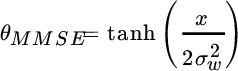
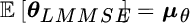
In information theory this is referred as soft decoding. Figure 11.4 shows the non‐linearity that represents the MMSE estimate θMMSE from the observation x. For a low noise level (![]() ), the non‐linearity has the shape of a binary detector with threshold, while for high noise level (
), the non‐linearity has the shape of a binary detector with threshold, while for high noise level (![]() ), the non‐linearity attains a linear behavior with a slope of
), the non‐linearity attains a linear behavior with a slope of ![]() . In fact, for
. In fact, for ![]() the noise dominates and the binary level that minimizes the MSE is 0 (i.e., halfway between the two choices). The MMSE estimation of w is based on the use of the non‐linearity that is complementary to the previous one considered, that for
the noise dominates and the binary level that minimizes the MSE is 0 (i.e., halfway between the two choices). The MMSE estimation of w is based on the use of the non‐linearity that is complementary to the previous one considered, that for ![]() coincides with the observation (as it is a 1:1 mapping).
coincides with the observation (as it is a 1:1 mapping).
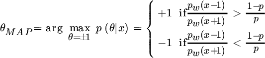
The MAP estimator should decide between two source values, and the decision among a limited set is part of detection theory, discussed later in Section 23.2. However, it is educational to use Bayesian inference to highlight the difference between MMSE and MAP in a non‐Gaussian context. The a‐posteriori pdf is:
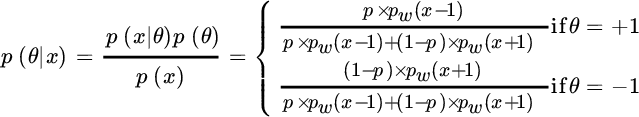
so the MAP is
![x vs. E[θ|x] with a sloping dash-dotted line and four solid lines representing σw= 0.1, σw= 1, σw= 0.5, and σw= 3.](http://images-20200215.ebookreading.net/9/3/3/9781119293972/9781119293972__statistical-signal-processing__9781119293972__images__c11f004.gif)
Figure 11.4 MMSE estimator for binary valued signals.
Since
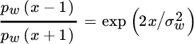
the MAP estimator reduces to
which for ![]() (the most common case in digital communications) is
(the most common case in digital communications) is ![]() . It is without doubt that MMSE and MAP are clearly different from one another: the MMSE estimate returns a value that is not compatible with the generation mechanism but still has minimum MSE; the MAP estimate is simply the decision between the two alternative hypotheses
. It is without doubt that MMSE and MAP are clearly different from one another: the MMSE estimate returns a value that is not compatible with the generation mechanism but still has minimum MSE; the MAP estimate is simply the decision between the two alternative hypotheses ![]() or
or ![]() (see Chapter 23).
(see Chapter 23).
11.1.4 Example: Impulse Noise Mitigation
In real life, the stationarity assumption of Gaussian noise (or any other stochastic process) is violated by the presence of another phenomenon that occurs unexpectedly with low probability but large amplitudes: this is impulse noise. Gaussian mixtures can be used to model impulse noise that is characterized by long tails in the pdf (like those generated by lightning, power on/off, or other electromagnetic events) and it was modeled this way by Middleton in 1973. Still referring to the observation model ![]() , the rv labeled as “noise” is θ while w is the signal of interest (just to use a notation congruent with all above) with a Gaussian pdf.
, the rv labeled as “noise” is θ while w is the signal of interest (just to use a notation congruent with all above) with a Gaussian pdf.
The value of the random variable θ is randomly chosen between two (or more) values associated to two (or more) different random variables. Therefore the random variable θ can be expressed as

and its pdf is the mixture
that is a linear combination of the pdfs associated to the two random variables α e β. The pdf of the observation is the convolution of the θ and w pdfs:
and this can be used to obtain (from (11.1)) the MMSE estimator of θ or w in many situations.
The Gaussian mixture with ![]() and
and ![]() can be shaped to model the tails of the pdf; for zero‐mean (
can be shaped to model the tails of the pdf; for zero‐mean (![]() ) Gaussians, the pdf is:
) Gaussians, the pdf is:

Figure 11.5 Example of data affected by impulse noise (upper figure), and after removal of impulse noise (lower figure) by MMSE estimator of the Gaussian samples (back line) compared to the true samples (gray line).
The MMSE estimator for x is
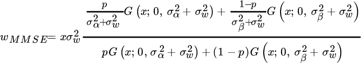
The effect of “spiky” data is illustrated in Figure 11.5 with x affected by Gaussian noise and some impulse noise. The estimated MMSE wMMSE compared to true w (gray line) shows a strong reduction of non‐Gaussian (impulse) noise but still leaves the Gaussian noise that cannot be mitigated from a non‐linear MMSE estimator other than by filtering as is discussed later (simulated experiment with ![]() ,
, ![]() and
and ![]() ). Namely, the noise with large amplitude, when infrequently present (
). Namely, the noise with large amplitude, when infrequently present (![]() ), is characterized by a Gaussian pdf with
), is characterized by a Gaussian pdf with ![]() , while normally there is little, or even no noise at all, as
, while normally there is little, or even no noise at all, as ![]() (
(![]() ). In this case the estimator has a non‐linearity with saturation that thresholds the observed values when too large compared to the background.
). In this case the estimator has a non‐linearity with saturation that thresholds the observed values when too large compared to the background.
Inspection of the MMSE estimator for varying parameters in Figure 11.6 shows that the threshold effect is more sensitive to the probability ![]() of large amplitudes rather than to their variance
of large amplitudes rather than to their variance ![]() (solid) and
(solid) and ![]() (dashed).
(dashed).
Figure 11.6 MMSE estimator for impulse noise modeled as Gaussian mixture.
11.2 Bayesian Estimation in Gaussian Settings
In general, Bayesian estimators are non‐linear and their derivation could be cumbersome, or prohibitively complex. When parameters and data are jointly Gaussian, the conditional pdf ![]() is Gaussian, and the MMSE estimator is a linear transformation of the observations. Furthermore, when the model is linear the MMSE estimator is very compact and in closed form. Even if the pdfs are non‐Gaussian and the MMSE estimator would be non‐linear, the use of a linear estimator in place of the true MMSE is very common and can be designed by minimizing the MSE. This is called a linear MMSE estimator (LMMSE), and in these situations the LMMSE is not optimal, but it has the benefit of being compact and pretty straightforward as it only requires knowledge of the first and second order central moments. For a Gaussian context, the LMMSE coincides with the MMSE estimator, and it is sub‐optimal otherwise.
is Gaussian, and the MMSE estimator is a linear transformation of the observations. Furthermore, when the model is linear the MMSE estimator is very compact and in closed form. Even if the pdfs are non‐Gaussian and the MMSE estimator would be non‐linear, the use of a linear estimator in place of the true MMSE is very common and can be designed by minimizing the MSE. This is called a linear MMSE estimator (LMMSE), and in these situations the LMMSE is not optimal, but it has the benefit of being compact and pretty straightforward as it only requires knowledge of the first and second order central moments. For a Gaussian context, the LMMSE coincides with the MMSE estimator, and it is sub‐optimal otherwise.
Tight lower bounds on the attainable MSE of the performance of any optimal or sub‐optimal estimation scheme are useful performance analysis tools for comparisons. The Bayesian CRB in Section 11.4 is the most straightforward extension of the CRB when parameters are random.
11.2.1 MMSE Estimator
The use of a Gaussian model for parameters and observations is very common and this yields a closed form MMSE estimator. Let p(x, θ) be joint Gaussian; then
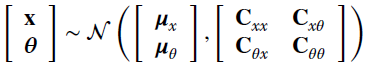
The conditional pdf ![]() is also Gaussian (see Section 3.5 for details and derivation):
is also Gaussian (see Section 3.5 for details and derivation):
This condition is enough to prove that the MMSE estimator is
which is linear after removing the a‐priori mean value μx from observations, and it has an elegant closed form.
In the additive noise model
the covariance matrixes and the mean values lead to the following results (under the hypothesis that w and θ are mutually uncorrelated):
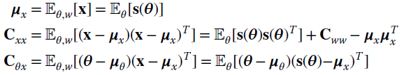
Note that moments wrt the parameters ![]() are the only new quantities to be evaluated to derive the MMSE estimator. When the model s(θ) is linear, the central moments are further simplified as shown below.
are the only new quantities to be evaluated to derive the MMSE estimator. When the model s(θ) is linear, the central moments are further simplified as shown below.
11.2.2 MMSE Estimator for Linear Models
The linear model with additive Gaussian noise is
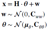
the moments can be related to the linear model H:

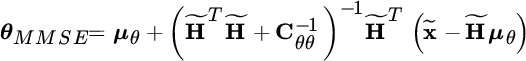
and the MMSE estimator is now
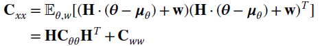
The covariance
is also useful to have the performance of the a‐posteriori method. Note that the a‐posteriori covariance is always an improvement over the a‐priori pdf, and this results from ![]() and thus
and thus
where the equality is when ![]() (i.e., data is not correlated with the parameters, and estimation of θ from x is meaningless).
(i.e., data is not correlated with the parameters, and estimation of θ from x is meaningless).
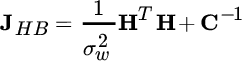
Computationally Efficient MMSE
There is a computational drawback in the MMSE method as the matrix ![]() has dimension
has dimension ![]() that depends on the size of the observations (N) and this could be prohibitively expensive as matrix inversion costs
that depends on the size of the observations (N) and this could be prohibitively expensive as matrix inversion costs ![]() . One efficient formulation follows from the algebraic properties of matrixes. Namely, the Woodbury identity
. One efficient formulation follows from the algebraic properties of matrixes. Namely, the Woodbury identity ![]() (see Section 1.1.1) can be applied to the linear transformation in MMSE expression:
(see Section 1.1.1) can be applied to the linear transformation in MMSE expression:
This leads to an alternative formulation of the MMSE estimator:
This expression is computationally far more efficient than (11.2) as the dimension of ![]() is
is ![]() , and the number of parameters is always smaller than the number of measurements (
, and the number of parameters is always smaller than the number of measurements (![]() ); hence the MMSE estimator (11.4) has a cost
); hence the MMSE estimator (11.4) has a cost ![]()
![]() .
.
Moreover, the linear transformation ![]() can be evaluated in advance as a Cholesky factorization of
can be evaluated in advance as a Cholesky factorization of ![]() and applied both to the regressor as
and applied both to the regressor as ![]() , and the observation x with the result of decorrelating the noise components (whitening filter, see Section 7.8.2) as
, and the observation x with the result of decorrelating the noise components (whitening filter, see Section 7.8.2) as ![]() with
with ![]() :
:
Example
The MMSE estimator provides a straightforward solution to the example of mean value estimate from multiple observations in Section 11.1.1 with model:
The general expression for the linear MMSE estimator is
After the Woodbury identity (Section 1.1.1) it is more manageable:
thus highlighting that the MMSE is the combination of the a‐priori mean value ![]() and the sample mean of the observations
and the sample mean of the observations ![]() , with
, with
For large N, the influence of noise decreases as ![]() , and for
, and for ![]() the importance of the a‐priori information decreases as
the importance of the a‐priori information decreases as ![]() , and
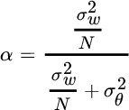
, and ![]() . Using the same procedure it is possible to evaluate
. Using the same procedure it is possible to evaluate
that is dependent on the weighting term α previously defined.
11.3 LMMSE Estimation and Orthogonality
The MMSE estimator ![]() can be complex to derive as it requires a detailed statistical model and the evaluation of the conditional mean
can be complex to derive as it requires a detailed statistical model and the evaluation of the conditional mean ![]() can be quite difficult, namely when involving non‐Gaussian rvs. A pragmatic approach is to derive a sub‐optimal estimator that is linear with respect to the observations and is based only on the knowledge of the first and the second order moments of the involved rvs. This is the the Linear MMSE (LMMSE) estimator, where the prefix “linear” denotes the structure of the estimator itself and highlights its sub‐optimality for non‐Gaussian contexts.
can be quite difficult, namely when involving non‐Gaussian rvs. A pragmatic approach is to derive a sub‐optimal estimator that is linear with respect to the observations and is based only on the knowledge of the first and the second order moments of the involved rvs. This is the the Linear MMSE (LMMSE) estimator, where the prefix “linear” denotes the structure of the estimator itself and highlights its sub‐optimality for non‐Gaussian contexts.
The LMMSE is based on the linear combination of N observations

while for the ensemble of p parameters it is
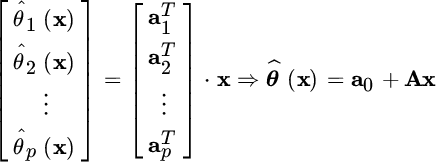
The estimator is based on the ![]() coefficients of matrix A that are obtained from the two constraints:
coefficients of matrix A that are obtained from the two constraints:
- Unbiasedness: from the Bayesian definition of bias (Section 6.3)
this provides a relationship for the scaling term

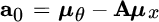
This term can be obtained by rewriting the estimator after the subtraction of the mean from both the parameters and the observations:

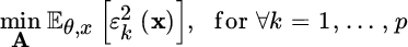
- MSE minimization: given the error
that corresponds to the k th parameter, one should minimize its mean square value

To simplify the notation it is assumed that the mean is subtracted from all the involved variables (in other words the assignment is
 and
and  ), or equivalently
  and
and  .
.Setting the gradients to zero:
This latter relationship is defined as the (statistical) orthogonality condition between the estimation error
 and the observations
or equivalently
By transposing both sides of the previous equation it is possible to write:
that shows how the orthogonality conditions lead to a set of N linear equations (one for each parameter θk) with N unknowns (the elements of the ak vector). The solution of this set of equation is given by (recall the assumptions here:
 ,
,  , or
, or  )(11.7)
Generalizing the orthogonality conditions between observations and estimation error:

which corresponds to pN equations into the pN unknowns entries of A. Substituting the estimator relationship
 into the previous equation yields the LMMSE estimator:(11.8)
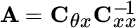
Considering now also the relation to zeroing the polarization, it is possible to write the general expression for the LMMSE estimator:

that obviously gives
 .
.The dispersion of the estimate is by the covariance:

and the fundamental relationships of LMMSE are the same as for the MMSE for Gaussian models in Section 11.2.1.
Figure 11.7 Geometric view of LMMSE orthogonality.
Compared to the general MMSE, that is never simple or linear, any LMMSE estimator is based on the moments that should be known, and the cross‐covariance matrix Cθx between the observations and the parameters. This implies that the LMMSE estimator can always be derived in closed form, but it has no proof of optimality. However, it is worthwhile to remark that the LMMSE coincides with the MMSE estimator for Gaussian variables, and it is the optimum MMSE estimator in this situation. The linear MMSE (LMMSE) estimator provides a sub‐optimal estimation in the case of random variables with arbitrary pdfs even if it provides the estimation with the minimum MSE among all linear estimators. The degree of sub‐optimality follows from the analysis of the covariance matrix cov[θLMMSE], which for the sub‐optimal case (non‐Gaussian pdfs) has a larger value with respect to the “true” (optimal) MMSE estimation. In summary:
(the difference is semipositive definite). The simplicity of the LMMSE estimator justifies its wide adoption in science and engineering, and sometimes the optimal MMSE is so complex to derive that the LMMSE is referred to (erroneously!) as the MMSE estimator.
Orthogonality
The orthogonality condition between the observations x and the estimation errors ![]() states that these are mutually orthogonal
states that these are mutually orthogonal

This is the general way to derive the LMMSE estimator as the set of Np equations that are enough to derive the ![]() entries of A. The representation
entries of A. The representation
decomposes the vector θ into two orthogonal components as

This relation is also called Pitagora’s statistical theorem, illustrated geometrically in Figure 11.7.
11.4 Bayesian CRB
When MMSE estimators are not feasible, or practical, the comparison of any estimator with lower bounds is a useful performance index. Given any Bayesian estimator g(x), the Bayesian MSE is
where the right hand side is the conditional mean estimator that has the minimum MSE over all possible estimators. The Bayesian CRB was introduced in the mid‐1960s by Van Trees [37,42] and it states that under some regularity conditions
where
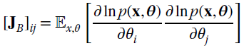
Since ![]() , the Bayesian CRB is the sum of two terms:
, the Bayesian CRB is the sum of two terms:
where

is the contribution of data that can be interpreted as the mean of the FIM for non‐Bayesian estimators (Section 8.1) over the distribution of parameters, and
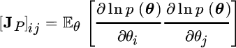
is the contribution of the a‐priori information.
In detail, the MSE bound of any Bayesian estimator can be stated as follows:

with equality only if the a‐posteriori pdf ![]() is Gaussian. The condition for Bayesian CRB to hold requires that the estimate is unbiased according to the Bayesian context
is Gaussian. The condition for Bayesian CRB to hold requires that the estimate is unbiased according to the Bayesian context
which is evaluated for an average choice of parameters according to their pdf p[θ]. This unbiasedness condition for a random set of parameters is weaker than the CRB for deterministic parameters, which needs to be unbiased for any choice of θ. Further inspection shows that (Section 1.1.1)
where J(θ) is the FIM for non‐Bayesian case (Chapter 8).
11.5 Mixing Bayesian and Non‐Bayesian
The Bayesian vs. non‐Bayesian debate is a long‐standing one. However, complex engineering problems are not always so clear— the a‐priori pdf is not known, or a‐priori information is not given as a pdf, and the parameters could mix nuisance, random, and deterministic ones. Making a set of cases, exceptions, and examples with special settings could take several pages, and the reader would feel disoriented faced with a taxonomy. Other than to warn the reader that one can be faced with a complex combination of parameters, the recommendation is to face the problems with a cool head using all the analytical tools discussed so far, and mix them as appropriate.
11.5.1 Linear Model with Mixed Random/Deterministic Parameters
Let the linear model with mixed parameters be:
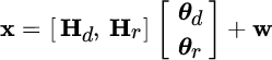
where θd is deterministic, and the other set θr is random and Gaussian
This is the called hybrid estimation problem. Assuming that the noise is ![]() , one can write the joint pdf
, one can write the joint pdf ![]() ; under the Gaussian assumption of terms, the logarithmic of the pdf is
; under the Gaussian assumption of terms, the logarithmic of the pdf is

and the MAP/ML estimator is obtained by setting
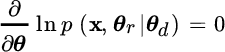
for random (θr) and deterministic (θd) parameters, and every x. The log‐pdf can be rewritten more compactly as

where for analytical convenience it is defined that

The gradient becomes

where the joint estimate is

The CRB for this hybrid system is [43] (Section 11.5.2)
where
Example: A sinusoid has random amplitude sine/cosine components (this generalizes the case of deterministic amplitude in Section 9.2). From Section 5.2, the model is
with
The log‐pdf for random α is

that minimized wrt to α for a given ω yields:
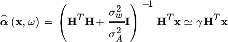
Since ![]() :
:

This estimate ![]() substituted into the log‐pdf (neglecting scale‐factors)
substituted into the log‐pdf (neglecting scale‐factors)

proves that, regardless of whether the amplitude is deterministic or modeled as stochastic Gaussian, the frequency estimate is the value that maximizes the amplitude of the Fourier transform as for the MLE in Section 9.2, and Section 9.3.
11.5.2 Hybrid CRB
The case when the parameters are mixed non‐random and random needs a separate discussion. Let

be the ![]() parameters grouped into
parameters grouped into ![]() non‐random θd, and
non‐random θd, and ![]() random θr, the MSE hybrid bound is obtained from the pdf [37]
random θr, the MSE hybrid bound is obtained from the pdf [37]
that decouples random and non‐random parameters. The Hybrid CRB
where
is now partitioned with expectations over θr


The random parameters θr can be nuisance, and the Hybrid CRB on deterministic parameters θd is less tight than the CRB for the same parameters [43].
Figure 11.8 Mapping between complete  and incomplete (or data)
  set in EM method.
11.6 Expectation‐Maximization (EM)
Making reference to non‐Bayesian methods in Chapter 7, the MLE of the parameters θ according to the set of observations x is
However, it could happen that the optimization of the log‐likelihood function is complex and/or not easily tractable, and/or it depends on too many parameters to be easily handled. The expectation maximization algorithm [45] solves the MLE by postulating that there exists a set of alternative observations y called complete data so that it is always possible to get the “true” observations x (here referred as incomplete data) from a not‐invertible transformation (i.e., many‐to‐one) ![]() . The new set y is made in such a way that the MLE wrt the complete set
. The new set y is made in such a way that the MLE wrt the complete set ![]() is better constrained and much easier to use, and/or computationally more efficient, or numerical optimization is more rapidly converging.
is better constrained and much easier to use, and/or computationally more efficient, or numerical optimization is more rapidly converging.
The choice of the set y (and the transformation γ(.)) is the degree of freedom of the method and is arbitrary, but in any case it cannot be inferred from the incomplete set as the transformation is not‐invertible. The EM algorithm alternates the estimation (expectation or E‐step) of the log‐likelihood ![]() from the observations x (available), and the estimate θ(n) (at n th iteration) from the maximization (M‐step) from the estimate of
from the observations x (available), and the estimate θ(n) (at n th iteration) from the maximization (M‐step) from the estimate of ![]() . More specifically, the log‐likelihood
. More specifically, the log‐likelihood ![]() is estimated using the MMSE approach given (x, θ(n)); this is the expected mean estimate, and the two steps of the EM algorithm are
is estimated using the MMSE approach given (x, θ(n)); this is the expected mean estimate, and the two steps of the EM algorithm are

The E‐step is quite simple in the case that the model has additive Gaussian noise and the transformation γ(.) is linear but still not‐invertible; this case is discussed in detail below.
The EM method converges to a maximum, but not necessarily the global maximum. In any case, it can be proved that, for any choice θ(n) that corresponds to the solution at the nth iteration, the inequality ![]() holds for any choice
holds for any choice ![]() , and the corresponding likelihood for the MLE is always increasing:
, and the corresponding likelihood for the MLE is always increasing: ![]() .
.
11.6.1 EM of the Sum of Signals in Gaussian Noise
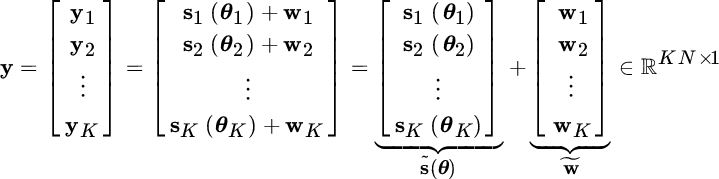
The derivation here has been adapted from the original contribution of Feder and Weinstein, 1988 [46] for superimposed signals in Gaussian noise. Let the observation ![]() be the sum of K signals each dependent on a set of parameters:
be the sum of K signals each dependent on a set of parameters:

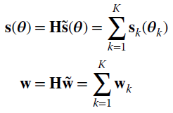
where sk(θk) is the k th signal that depends on the k th set of parameters θk and ![]()
![]() . The objective is to estimate all the set of parameters
. The objective is to estimate all the set of parameters ![]() from the observations by decomposing the superposition of K signals s(θ) into K simple signals, all by using the EM algorithm.
from the observations by decomposing the superposition of K signals s(θ) into K simple signals, all by using the EM algorithm.
The complete set from the incomplete x is based on the structure of the problem at hand. More specifically, one can choose as a complete set the collection of each individual signal:
where the incomplete set is the superposition of the signals
where ![]() is the non‐invertible transformation γ(y). The following conditions should hold to preserve the original MLE:
is the non‐invertible transformation γ(y). The following conditions should hold to preserve the original MLE:
To simplify the reasoning, each noise term in the complete set is assumed as uncorrelated wrt the others (![]() for
for ![]() ), but with the same correlation properties of w except for an arbitrary scaling
), but with the same correlation properties of w except for an arbitrary scaling
so that
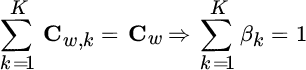
To summarize, the noise of the complete set is
and the ![]() covariance matrix is block‐diagonal
covariance matrix is block‐diagonal
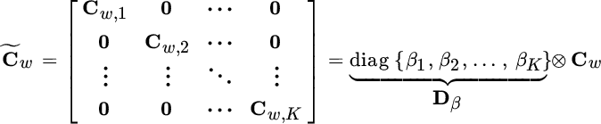
so it is convenient and compact (but not strictly necessary) to use the Kronecker products notation (Section 1.1.1). The inverse ![]() is still block‐diagonal. From the pdf of
is still block‐diagonal. From the pdf of ![]() for the complete set:
for the complete set:
and the log‐likelihood is (up to a scaling factor)

Computing the conditional mean ![]() gives (apart from a scaling term
gives (apart from a scaling term ![]() that is independent of θ)
that is independent of θ)
where ![]() is the Bayesian estimate of the complete set from the incomplete x and current estimate θ(n). For the optimization wrt θ (M‐step), it is convenient to group the terms of
is the Bayesian estimate of the complete set from the incomplete x and current estimate θ(n). For the optimization wrt θ (M‐step), it is convenient to group the terms of ![]() after adding/removing the term
after adding/removing the term ![]() as independent of θ:
as independent of θ:
where c, d, e are scaling terms independent of θ.
The estimation of the complete set ![]() is based on the linear model
is based on the linear model
and thus on the basis of the transformation ![]() . The MMSE estimate of y from the incomplete observation set (the only one available) x for Gaussian noise (here equal to zero) is4
. The MMSE estimate of y from the incomplete observation set (the only one available) x for Gaussian noise (here equal to zero) is4
The terms of the estimate ŷ(θ(n)) can be expanded by using the property of Kronecker products (Section 1.1.1)
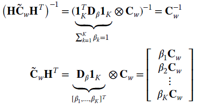
substituting and simplifying, it follows that the MMSE estimate of the k th signal of the complete set at the n‐th iteration of the EM method is

which is the sum of the k th signal estimated from the parameter ![]() at the n‐th iteration and the original observation x after stripping all the signals estimated up to the n‐th iteration and interpreted as noise, and thus weighted for the corresponding scaling term βk. Re‐interpreting
at the n‐th iteration and the original observation x after stripping all the signals estimated up to the n‐th iteration and interpreted as noise, and thus weighted for the corresponding scaling term βk. Re‐interpreting ![]() now, it can be seen that
now, it can be seen that

or equivalently, the optimization is fragmented into a set of K local optimizations, one for each set of parameters (M‐step):

The model that uses the EM method for the superposition of signals in Gaussian noise is general enough to find several applications, such as for the estimation of the parameters for a sum of sinusoids as discussed in Section 10.4 for Doppler‐radar system, or a sum of waveforms (in radar or remote sensing systems), or the sum of pseudo‐orthogonal modulations (in spread‐spectrum and code division multiple access—CDMA—systems). An example of time of delay estimation is discussed below.
11.6.2 EM Method for the Time of Delay Estimation of Multiple Waveforms
Let the signal be the sum of K delayed echoes as in a radar system (Section 5.6); the waveform of each echo is known but not its amplitude and delay, and the ensemble of delays should be estimated from their superposition
Each waveform can be modeled as
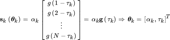
and the complete set of the EM method coincides with the generation model for each individual echo as if it were non‐overlapped with the others.
Given the estimate of amplitude ![]() and delay
and delay ![]() at then nth iteration, the two steps of the EM method are as follows.
at then nth iteration, the two steps of the EM method are as follows.
E‐step (for ![]() ):
):

M‐step (for ![]() ):
):

The M‐step is equivalent to the estimation of the delay of one isolated waveform from the signal ŷk(θ(n)) where the effect of the interference with the other waveforms has been (approximately) removed from the E‐Step (see Figure 11.9 with ![]() radar‐echoes). In other words, at every step the superposition of all the other waveforms (here in Figure 11.9 of the complementary waveform) is removed5 until (at convergence) the estimator of amplitude and delay acts on one isolated waveform and thus it is optimal. Of course, any imperfect cancellation of other waveforms could cause the EM method to converge to some local maximum. This problem is not avoided at all by the EM method and should be verified case‐by‐case.
radar‐echoes). In other words, at every step the superposition of all the other waveforms (here in Figure 11.9 of the complementary waveform) is removed5 until (at convergence) the estimator of amplitude and delay acts on one isolated waveform and thus it is optimal. Of course, any imperfect cancellation of other waveforms could cause the EM method to converge to some local maximum. This problem is not avoided at all by the EM method and should be verified case‐by‐case.
Figure 11.9 ToD estimation of multiple waveforms by EM method ( ).
).
This example could be adapted for the estimation of frequency for sinusoids with different frequencies and amplitudes with small changes of terms, and the numerical example in Section 10.4 can suggest other applications of the EM method when trying to reduce the estimation of multiple parameters to the estimation of a few parameters carried out in parallel.
11.6.3 Remarks
The EM algorithm alternates the E‐step and the M‐step with the property that at every step the log‐likelihood function increases. However, there is no guarantee that convergence will be obtained to the global maximum, and the ability to reach convergence to the true MLE depends on the initialization θ(0) as for any iterative optimization method. Also, in some situations EM algorithm can be painfully slow to converge.
The mapping γ(.) that maps the incomplete set x from the complete (but not available) data y assumes that there are some missing measurements that complete the incomplete observations x. In some cases, adding these missing data can simplify the maximization of the log‐likelihood, but it could slow down the convergence of this EM method. Since the choice of the complete set is a free design aspect in the EM method, the convergence speed depends on how much information on the parameters are contained in the complete set.
Space‐alternating EM (SAGE) has been proposed in [47] to cope with the problem of convergence speed and proved to be successful in a wide class of application problems. A detailed discussion on this matter is left to publications specialized to solve specific applications by EM method.
Figure 11.10 Mixture model of non‐Gaussian pdfs.
Appendix Gaussian Mixture pdf
A non‐Gaussian pdf can be represented or approximated as a mixture of pdfs, mostly when multimodal, with long (or short) tail compared to a Gaussian pdf, or any combination thereof. Given some nice properties of estimators involving Gaussian pdfs, it can be convenient to rewrite (or approximate) a non‐Gaussian pdf as the weighted sum of Gaussian pdfs (Gaussian mixture) as follows (Figure 11.10):
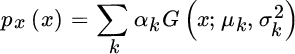
Parameters ![]() characterize each Gaussian function used as the basis of the Gaussian mixture, and {αk} are the mixing proportions constrained by
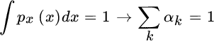
characterize each Gaussian function used as the basis of the Gaussian mixture, and {αk} are the mixing proportions constrained by ![]() . The problem of finding the set of parameters
. The problem of finding the set of parameters ![]() that better fits the non‐Gaussian pdf is similar to interpolation over non‐uniform sampling with one additional constraint on pdf normalization
that better fits the non‐Gaussian pdf is similar to interpolation over non‐uniform sampling with one additional constraint on pdf normalization
Methods to get the approximating parameters ![]() are many, and the method of moments (MoM) is a simple choice if either px(x) is analytically known, or a set of samples {xℓ} are available. Alternatively, one can assume that the Gaussian mixture is the data generated from a set of independent and disjoint experiments, and one can estimate the parameters by assigning each sample to each of the experiments, as detailed in Section 23.6.
are many, and the method of moments (MoM) is a simple choice if either px(x) is analytically known, or a set of samples {xℓ} are available. Alternatively, one can assume that the Gaussian mixture is the data generated from a set of independent and disjoint experiments, and one can estimate the parameters by assigning each sample to each of the experiments, as detailed in Section 23.6.
To generate a non‐Gaussian process x[n] with Gaussian mixture pdf based on K Gaussian functions, one can assume that there are K independent Gaussian generators (y1, y2, …, yK) each with ![]() , and the assignment
, and the assignment ![]() is random with mixing probability αk and it is mutually exclusive wrt the others. A simple example here can help to illustrate. Let
is random with mixing probability αk and it is mutually exclusive wrt the others. A simple example here can help to illustrate. Let ![]() be the number of normal rvs; the Gaussian mixture is obtained by selecting each sample out of three Gaussian sources, with selection probability {α1, α2, α3} into the
be the number of normal rvs; the Gaussian mixture is obtained by selecting each sample out of three Gaussian sources, with selection probability {α1, α2, α3} into the ![]() vector
vector alfa:
The generalization to N‐dimensional Gaussian mixture pdf is straightforward:

The central moments {μk, Ck} are the generalization to N rvs of the Gaussian mixture (11.9).