
23
Classification and Clustering
There are many applications where a set of data should be classified as belonging to a predefined subset, or to discover the structure of the data when those subsets are not known. In signal processing, a signal can contain or not a specific waveform, or an image can be contain or not a feature of interest (e.g., a search for faces in images), or feature extraction can be used to reduce the complexity of the image itself. This chapter covers methods for classification and clustering as part of routine statistical signal processing for signal detection or feature extraction. The topic is broad, and the focus is to discuss the essential concepts collected in Table 23.1.
Table 23.1 Taxonomy of principles and methods for classification and clustering.
| Classification (Section 23.2) | Clustering (Section 23.6) | |
| Prior knowledge | No a‐priori classes and numbers | |
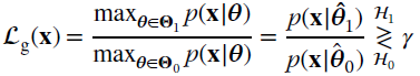
| p( |
||
| Application | Classify new sample x into |
Grouping of homogeneous data |
| (structure discovery from data) | ||
| Methods | Detection theory (Section 23.2.1) | K‐means and EM clustering |
| Bayesian classifiers (Section 23.4) | ||
| Metric | Classification probability | Minimum clusters/clustering error |
Classification involves the identification of group membership and it can be quantitatively stated using an example from handwriting recognition. Consider the handwritten images that correspond to each of the digits 0,1,…,9 indicated as classes; each image is digitized into a set of N pixels that form the observation vector ![]() . The final goal is to have a classifier that identifies which digit corresponds to a certain x knowing the features of all the classes. In a classification problem, the parametric pdfs
. The final goal is to have a classifier that identifies which digit corresponds to a certain x knowing the features of all the classes. In a classification problem, the parametric pdfs ![]() for the K classes
for the K classes ![]() 1,
1, ![]() 2, …,
2, …, ![]() K are known from the problem settings and are used for the decision of x in favor of the class that maximizes the probability
K are known from the problem settings and are used for the decision of x in favor of the class that maximizes the probability ![]() , as for maximum likelihood. Whenever the pdfs
, as for maximum likelihood. Whenever the pdfs ![]() are not known either in closed form or analytically, one can use a set of training data to infer these properties from experiments, and let the classifier learn from samples (e.g., the classifier learns the main features from a training sample of handwritten digits, and any new x is classified based on the features extracted from the training set); this is called supervised learning.
are not known either in closed form or analytically, one can use a set of training data to infer these properties from experiments, and let the classifier learn from samples (e.g., the classifier learns the main features from a training sample of handwritten digits, and any new x is classified based on the features extracted from the training set); this is called supervised learning.
Classification when ![]() is binary between two alternative hypotheses of the data. This problem has been widely investigated in the statistical signal processing literature and it is the basis of understanding more evolved classification methods with
is binary between two alternative hypotheses of the data. This problem has been widely investigated in the statistical signal processing literature and it is the basis of understanding more evolved classification methods with ![]() (also called multiple hypothesis testing).
(also called multiple hypothesis testing).
In Bayesian classification, each of the classes is characterized by the corresponding a‐priori probability p(![]() 1), p(
1), p(![]() 2), …, p(
2), …, p(![]() K), and the joint pdf
K), and the joint pdf ![]() gives the complete probabilistic description of the problem at hand. Bayes’ theorem for classification
gives the complete probabilistic description of the problem at hand. Bayes’ theorem for classification

is instrumental in getting the a‐posteriori probability for each class, and this is useful to decide to use a‐posteriori probability criteria that assign x to the class with the largest a‐posteriori probability ![]() . The classification metric is the correct or incorrect classification probability:
. The classification metric is the correct or incorrect classification probability:
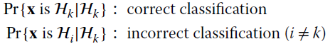
or any other error probability that accounts for all the wrong (Section 23.2.1).
When classification involves signals, it is called detection theory and good references are [128,132,37]. Classification is the basis of pattern recognition, and overviews are provided by Fukunaga [129] and many others.
Clustering is the method of discovering any structure from a (large) set of samples {xℓ} when there is no a‐priori information on classes and no training is available (unsupervised learning). Cluster analysis divides data into groups (clusters) that are meaningful and/or useful, and the clusters should capture the natural structure of the data useful for a higher level of understanding. In signal processing, clustering is used to reduce the amount of information in signals, or to discover some properties of signals. Cluster analysis plays a key role when manipulating a large amount of data such as in pattern recognition, machine learning, and data mining. Application examples in the area of clustering aim to analyze and classify a large amount of data such as genetic information (e.g., genome analysis), multimedia information for information retrieval in the World Wide Web (which consists of billions of items of multimedia content), bank transactions to detect fraud, and business to segment customers into a small number of groups for additional analysis and marketing activities. An excellent review is by Jain [131], and a discussion of the application to learning processes in machine learning and mining of large data sets can be found in [142].
23.1 Historical Notes
Detection and classification in signal processing are two sides of the same coin. Signal detection algorithms decide whether a signal consists of “signal masked by noise” or “noise only,” and detection theory helps to design the algorithms that minimize the average number of decision errors. Detection and classification have their roots in statistical decision theory where they are called binary (![]() ) and K‐ary (
) and K‐ary (![]() ) hypothesis testing [124]. The first systematic developments in signal detection theory were around 1950 by communication and radar engineering [125,126], but some statistical detection algorithms were implemented even before that. From 1968, H. Van Trees [37] published a set of four volumes that are widely used in engineering, and vol. 3 is on detection theory [128], where he extensively investigated all the possible cases of signal detection with/without known parameters/noise/signals, as briefly revised herein.
) hypothesis testing [124]. The first systematic developments in signal detection theory were around 1950 by communication and radar engineering [125,126], but some statistical detection algorithms were implemented even before that. From 1968, H. Van Trees [37] published a set of four volumes that are widely used in engineering, and vol. 3 is on detection theory [128], where he extensively investigated all the possible cases of signal detection with/without known parameters/noise/signals, as briefly revised herein.
In general, classification in statistical signal processing problems is: (1) classifying an individual waveform out of a set of waveforms that could be linearly independent to form a basis, or (2) classifying the presence of a particular set of signals as opposed to other sets of signals, and classifying the number of signals present. Each of these problems are based on the definition of specific classes that depend on the specific signals at hand.
In pattern recognition, classification is over a set of classes. Classification for multivariate Normal distributions was proposed by Fisher in 1936 [133] with a frequentist vision, and the target is to use a linear transformation that set the basis for linear discriminant analysis (LDA). The characteristics of the classes are known, and the aim is to establish a rule whereby we can classify a new observation into one of the existing classes. The classification rule can be defined by well‐defined statistical properties of the data or, in complex contexts, the classifier can be trained by using some known data–class pairs. Pattern recognition dates back to around 1967 when it was established as a dedicated Technical Committee by the IEEE Computer Society; a comprehensive book by K. Fukunaga appeared in 1972 [127], while the first dedicated IEEE journal appeared in 1979. There are many applications based on the recognition of patterns such as handwriting and optical character recognition, speech recognition, image recognition, and information retrieval, just to mention a few. Classification rules in all these applications are based on a preliminary training—supervised training is part of the machine learning process. Machine Learning is the field of study that gives computers the ability to learn without being explicitly programmed (this definition is attributed to A. Samuel, 1959) [130], and nowadays it is synonymous with pattern recognition. In this framework, neural networks are a set of supervised algorithms that achieve classification using the connection of a large number of simple threshold‐based processors.
Clustering methods to infer the structure of data from the data itself (unsupervised learning) are of broad interest since the early paper by J. MacQueen in 1967 [141], and the use of mixture models for clustering [134] [143] strengthen their performance.
23.2 Classification
23.2.1 Binary Detection Theory
The two‐group (or binary) classification problem between two classes indexed as ![]() 0 and
0 and ![]() 1 was largely investigated in the past as being the minimal classification. Detection theory in signal processing is used to decide if x contains a signal + noise or just noise, and this is a typical problem in conventional radar systems (Section 5.6) where it is crucial to detect or not the presence of a target. In communication engineering, binary classification is used to decide if a transmitted bit is 0 or 1 (Section 17.1), or if the frequency of a sinusoid is ω0 or ω1 provided that the class of frequencies are {ω0, ω1}, just to mention few. Furthermore, in medicine, binary classification is used to decide if a patient is healthy or not, in bank or electronic payments if transactions are secure or not, in civil engineering if a bridge is faulty or not, etc.
1 was largely investigated in the past as being the minimal classification. Detection theory in signal processing is used to decide if x contains a signal + noise or just noise, and this is a typical problem in conventional radar systems (Section 5.6) where it is crucial to detect or not the presence of a target. In communication engineering, binary classification is used to decide if a transmitted bit is 0 or 1 (Section 17.1), or if the frequency of a sinusoid is ω0 or ω1 provided that the class of frequencies are {ω0, ω1}, just to mention few. Furthermore, in medicine, binary classification is used to decide if a patient is healthy or not, in bank or electronic payments if transactions are secure or not, in civil engineering if a bridge is faulty or not, etc.
The binary decision is based on the choice between two hypotheses referred as the null hypothesis ![]() 0 and the alternative hypothesis
0 and the alternative hypothesis ![]() 1, and for the case of known pdfs the associated pdfs are
1, and for the case of known pdfs the associated pdfs are ![]() and
and ![]() . The decision criterion on x is based on certain disjoint decision regions
. The decision criterion on x is based on certain disjoint decision regions ![]() 0 and
0 and ![]() 1, such that
1, such that ![]() . The decision regions are tailored according to the decision metric, and an intuitive one is to decide in favor of
. The decision regions are tailored according to the decision metric, and an intuitive one is to decide in favor of ![]() 1 if
1 if ![]() , and for
, and for ![]() 0 if
0 if ![]() as for maximum likelihood criteria. Since decision regions do not involve any statistical comparison on actual data, but rather the design of the regions to be used according to the decision metric, regions are more practical in decision between
as for maximum likelihood criteria. Since decision regions do not involve any statistical comparison on actual data, but rather the design of the regions to be used according to the decision metric, regions are more practical in decision between ![]() 0 vs.
0 vs. ![]() 1 yet recognizing the equivalence of comparing
1 yet recognizing the equivalence of comparing ![]() vs.
vs. ![]() .
.
Any value x is classified as ![]() 0 if it belongs to
0 if it belongs to ![]() 0 (
0 (![]() , and
, and ![]() ), and alternatively is classified as
), and alternatively is classified as ![]() 1 if it belongs to
1 if it belongs to ![]() 1 (
1 (![]() , and
, and ![]() ). Correct classification is when
). Correct classification is when ![]() and the true class is
and the true class is ![]() 1, and this is indicated as a true positive (TP). Conversely, a true negative (TN) is for
1, and this is indicated as a true positive (TP). Conversely, a true negative (TN) is for ![]() and the true class is
and the true class is ![]() 0. One can define the probability for TP and TN as indicated in Table 23.2. Misclassification is when
0. One can define the probability for TP and TN as indicated in Table 23.2. Misclassification is when ![]() and the true class is
and the true class is ![]() 0, this is called a false positive (FP), and when
0, this is called a false positive (FP), and when ![]() and the true class is
and the true class is ![]() 1, a false negative (FN). An alternative notation used here comes from radar contexts (but applies also to tumor detection) where
1, a false negative (FN). An alternative notation used here comes from radar contexts (but applies also to tumor detection) where ![]() 1 refers to a target (that is important to detect with minimal error), and
1 refers to a target (that is important to detect with minimal error), and ![]() 0 is the lack of any target: TP is true target detection, and FP is a false alarm when there is no target. Table 23.2 summarizes the cases, however statisticians uses a different notation in binary hypothesis testing: sensitivity is TP probability
0 is the lack of any target: TP is true target detection, and FP is a false alarm when there is no target. Table 23.2 summarizes the cases, however statisticians uses a different notation in binary hypothesis testing: sensitivity is TP probability ![]() , specificity is TN probability
, specificity is TN probability ![]() .
.
Table 23.2 Classification metrics.
| True hypothesis | ||
| Decision on x | ||
The shape of the decision regions ![]() 0 and
0 and ![]() 1 for test hypothesis
1 for test hypothesis ![]() 0 versus
0 versus ![]() 1 depends on the classification metrics that are based on the probabilities
1 depends on the classification metrics that are based on the probabilities
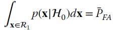
The probability of a false alarm (also called size of test in statistics) is (Figure 23.1)
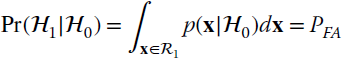
and measures the worst‐case probability of choosing ![]() 1 when
1 when ![]() 0 is in place. Detection probability (Figure 23.1)
0 is in place. Detection probability (Figure 23.1)

measures the probability of correctly accepting ![]() 1 when
1 when ![]() 1 is in force. Since
1 is in force. Since ![]() and
and ![]() , any complementary probability is fully defined from the pair PD and PFA. The goal is to choose the test
, any complementary probability is fully defined from the pair PD and PFA. The goal is to choose the test

or equivalently the decision region boundary, to have the largest PD with minimum PFA. These probabilities cannot be optimized together, and conventionally one constrains ![]() and chooses the largest PD. This is the celebrated Neyman–Pearson (NP) test that is obtained by solving the optimization constraining
and chooses the largest PD. This is the celebrated Neyman–Pearson (NP) test that is obtained by solving the optimization constraining ![]() from the Lagrangian:
from the Lagrangian:
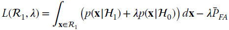
Figure 23.1 Binary hypothesis testing.
To maximize L(![]() 1, λ), the argument should be
1, λ), the argument should be ![]() within the decision bound
within the decision bound ![]() 1, and this is the basis for the proof that shows that
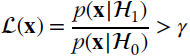
1, and this is the basis for the proof that shows that ![]() (see e.g., [132] for details). The decision is based on the likelihood ratio
(see e.g., [132] for details). The decision is based on the likelihood ratio ![]() and the decision in favor of
and the decision in favor of ![]() 1 is called the likelihood ratio test (LRT)
1 is called the likelihood ratio test (LRT)
(or alternatively, decide ![]() 0 if
0 if ![]() ), where the threshold
), where the threshold ![]() is obtained by solving for the constraint
is obtained by solving for the constraint
The LRT is often indicated by highlighting the two alternative selections wrt the threshold:
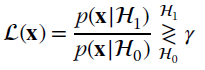
The notation compactly specifies that for ![]() , the decision is in favor of
, the decision is in favor of ![]() 1 and for
1 and for ![]() it is for
it is for ![]() 0. The NP‐test solves for the maximum PD constrained to a certain PFA, and the corresponding value of optimized PD vs. PFA can be evaluated analytically for the optimum threshold values. The plot of (optimized) PD vs. PFA (or equivalently sensitivity vs. 1‐specificity) is called the receiver operating characteristic (ROC), and it represents a common performance indicator of test statistics that removes the dependency on the threshold. The analysis of the ROC curve reveals many properties of the specific decision rule of
0. The NP‐test solves for the maximum PD constrained to a certain PFA, and the corresponding value of optimized PD vs. PFA can be evaluated analytically for the optimum threshold values. The plot of (optimized) PD vs. PFA (or equivalently sensitivity vs. 1‐specificity) is called the receiver operating characteristic (ROC), and it represents a common performance indicator of test statistics that removes the dependency on the threshold. The analysis of the ROC curve reveals many properties of the specific decision rule of ![]() 1 versus
1 versus ![]() 0 based on the statistical properties
0 based on the statistical properties ![]() versus
versus ![]() that are better illustrated by an example from [128].
that are better illustrated by an example from [128].
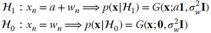
Example: Detection of a Constant in Uncorrelated Noise
Assume that the signal is represented by a constant amplitude ![]() in Gaussian noise (value of a is known but not its presence), and one should decide if there is a signal or not by detecting the presence of a constant amplitude in a set of N samples
in Gaussian noise (value of a is known but not its presence), and one should decide if there is a signal or not by detecting the presence of a constant amplitude in a set of N samples ![]() . This introductory example is to illustrate the steps to produce the corresponding ROC curves. The two alternative hypotheses for the signal x are
. This introductory example is to illustrate the steps to produce the corresponding ROC curves. The two alternative hypotheses for the signal x are
The LRT is

which in this case it simplifies as
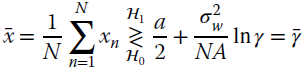
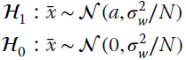
The test is based on the sample mean of the signal, which can be considered as an estimate of the amplitude (Section 7.2). Since the PD vs. PFA analysis depends on the pdf of the sample mean ![]() under the two hypotheses, these should be detailed based on the properties of the LRT manipulations. In this case, since decision statistic
under the two hypotheses, these should be detailed based on the properties of the LRT manipulations. In this case, since decision statistic ![]() is the sum of Gaussians, the pdfs for the two conditions are:
is the sum of Gaussians, the pdfs for the two conditions are:
and the probabilities can be evaluated analytically vs ![]()


where the Q‐function

is monotonic decreasing with increasing ς. The probabilities are monotonic decreasing with the threshold ![]() ranging from
ranging from ![]() for
for ![]() (i.e., accept any condition as being
(i.e., accept any condition as being ![]() , even if wrong) down to
, even if wrong) down to ![]() for
for ![]() (i.e., reject any condition as being
(i.e., reject any condition as being ![]() , even if wrong), but in any case the probabilities
, even if wrong), but in any case the probabilities ![]() are useless as this implies that decision
are useless as this implies that decision ![]() 1 vs
1 vs ![]() 0 is random, or equivalently the two hypotheses are indistinguishable (i.e.,
0 is random, or equivalently the two hypotheses are indistinguishable (i.e., ![]() ).
).
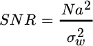
To derive the ROC, consider a given PFA; one can optimally evaluate the threshold γ that depends on the signal to noise ratio
and the corresponding PD is the largest one subject to the PFA. The ROC is independent of the threshold ![]() , which should be removed from the dependency of PFA in (23.2) using the inverse Q‐function:
, which should be removed from the dependency of PFA in (23.2) using the inverse Q‐function: ![]() . Plugging this dependency into the PD:
. Plugging this dependency into the PD:
yields the locus of the optimal PD for a given PFA assuming that the test hypothesis is optimized. Figure 23.2 illustrates the ROC curve for different values of SNR showing that when the SNR value is small, the ROC curve is close to the random decision (dashed line), while for given PFA, the PD increases with SNR. The ROC curve is also the performance for the optimized threshold, and for the optimum decision regions that are here transformations of the observations.

Figure 23.2 Receiver operating characteristic (ROC) curves for varying SNR.
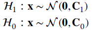
23.2.2 Binary Classification of Gaussian Distributions
The most general problem of binary classification between two Gaussian populations with known parameters can be stated as follows. Given the two classes
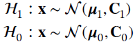
the decision rule becomes
Replacing the terms it follows that (apart from a constant)

and the decision boundary that divides the decision regions can be found for ![]()
![]() : it is quadratic in x and typically its shape is quite complex.
: it is quadratic in x and typically its shape is quite complex.
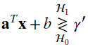
In the case where ![]() , the quadratic decision function degenerates into a linear one:
, the quadratic decision function degenerates into a linear one:
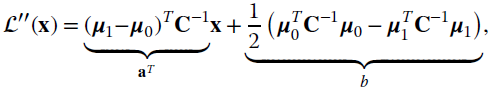
and the decision boundary is a hyperplane. Classification can be stated as finding the decision boundaries, and the number of parameters to define the quadratic decision function is ![]() while for the linear one it is
while for the linear one it is ![]() ; this is a convenience exploited in pattern analysis problems later in Section 23.5. The linear discriminant analysis (LDA) is based on the decision boundary
; this is a convenience exploited in pattern analysis problems later in Section 23.5. The linear discriminant analysis (LDA) is based on the decision boundary
that is adopted in pattern recognition, even when ![]() by using
by using
with weighting term α appropriately chosen [135,137].
The classification of Gaussian distributions is illustrated in the example in Figure 23.3 for ![]() with
with ![]() for
for ![]() . The decision boundary
. The decision boundary ![]() (gray line) between the two decision regions
(gray line) between the two decision regions ![]() 0 and
0 and ![]() 1 is linear. However, for the case
1 is linear. However, for the case ![]() that is here represented by the correlation
that is here represented by the correlation ![]() , the decision boundary for
, the decision boundary for ![]() is represented as a quadratic boundary, and the decision regions for
is represented as a quadratic boundary, and the decision regions for ![]() are multiple and their pattern is very complex for multidimensional (
are multiple and their pattern is very complex for multidimensional (![]() ) data.
) data.

Figure 23.3 Classification for Gaussian distributions: linear decision boundary for  (upper figure) and quadratic decision boundary for
  (lower figure).
To gain insight in the decision regions as a consequence of the tails of the Gaussians, Figure 23.4 shows the decision regions ![]() 0 and
0 and ![]() 1 for the case
1 for the case ![]() (line interval decision regions) and variances
(line interval decision regions) and variances ![]() .
.
Figure 23.4 Decision regions for  and
and  .
.
23.3 Classification of Signals in Additive Gaussian Noise
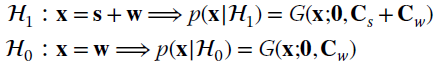
The general problem of signal classification in additive Gaussian noise can be stated for the two hypotheses:

with known (Section 23.3.1–23.3.3) or random (Section 23.3.4) signals s0, s1 and known Cw. Depending on the choice of the signals, this problem is representative of several common applications. The decision regions are linear and the decision criterion in closed form is (Section 23.2.2)

where the threshold γ collects all the problem‐specific terms for PD vs. PFA. The classification is part of the operations carried out by a receiving system that receives one of two alternative and known waveforms s1 and s0, or if the receiver should detect the presence of a backscattered waveform s1 in noise (when ![]() ). The performance of the decision is in terms of PD and PFA for a given threshold
). The performance of the decision is in terms of PD and PFA for a given threshold ![]() , and one can evaluate the statistical property of
, and one can evaluate the statistical property of ![]() that is Gaussian being the sum of Gaussian rvs under both hypotheses. These steps are the same as in Section 1, except analytically more complex, and one can evaluate the error probabilities PD and PFA in closed form, as well as the ROC.
that is Gaussian being the sum of Gaussian rvs under both hypotheses. These steps are the same as in Section 1, except analytically more complex, and one can evaluate the error probabilities PD and PFA in closed form, as well as the ROC.
23.3.1 Detection of Known Signal
In many applications such as radar/sonar or remote sensing systems, the interest is in detecting the presence (![]() 1) of a target that backscatters the transmitted (and known) waveform s or not (
1) of a target that backscatters the transmitted (and known) waveform s or not (![]() 0) in noisy data with known covariance Cw. Another context is in array processing with one active source (Section 19.1). The two hypotheses for the detection problem are
0) in noisy data with known covariance Cw. Another context is in array processing with one active source (Section 19.1). The two hypotheses for the detection problem are
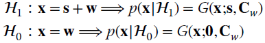
which is a special case with ![]() for
for ![]() 0. Incidentally, the example in Section 23.2.1 is a special case for the choice
0. Incidentally, the example in Section 23.2.1 is a special case for the choice ![]() and
and ![]() .
.
The detection rule is
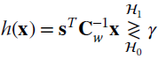
where the detector h(x) cross‐correlates the signal x with s, with a noise pre‐whitening by the ![]() . This is a generalized correlator–detector [128]. The pdf of h(x) under the two hypotheses is necessary to evaluate the ROC curve. The transformation h(x) is linear, and this simplifies the analysis as the rvs are Gaussian. In detail:
. This is a generalized correlator–detector [128]. The pdf of h(x) under the two hypotheses is necessary to evaluate the ROC curve. The transformation h(x) is linear, and this simplifies the analysis as the rvs are Gaussian. In detail:

and thus it is similar to (23.1, 23.2)

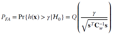
that yields the same PD vs. PFA in (23.3) provided that signal to nosie ratio is redefined as
Since the ROC curve moves upward when increasing SNR, the SNR can be maximized by a judicious choice s to conform to the covariance Cw. In detail, the choice ![]() where (λmin, qmin) is the minimum eigenvalue/eigenvector pair of Cw is optimal,
where (λmin, qmin) is the minimum eigenvalue/eigenvector pair of Cw is optimal, ![]() and this maximizes the SNR that in turn is
and this maximizes the SNR that in turn is ![]() .
.
This model can be specialized for detection of linear models (e.g., convolutive filtering, see Section 5.2) ![]() under
under ![]() 1 by simply re‐shaping the problem accordingly. The detector is
1 by simply re‐shaping the problem accordingly. The detector is ![]() , but since the MLE of θ is
, but since the MLE of θ is ![]() (Section 7.2.1), the detector (23.5) becomes
(Section 7.2.1), the detector (23.5) becomes
and the test hypothesis can be equivalently carried out on the estimates used as a sufficient statistic for θ without any performance loss.
23.3.2 Classification of Multiple Signals
In the case of multiple distinct signals in Gaussian noise, the model is

and classification is by identifying which hypothesis is more likely from the data. Assuming that all classes are equally likely with ![]() (see Section 23.4 how to generalize in any context), the decision in favor of
(see Section 23.4 how to generalize in any context), the decision in favor of ![]() k is when
k is when
Since inequalities hold for log‐transformations, it is straightforward to prove that the condition is
which is the hypothesis for the signal sk that is closest to x, where the distance is the weighted norm.
The case ![]() is common in communication engineering where the transmitter maps the information of a set of bits into one signal sk (modulated waveform) out of K, and the receiver must decide from a noisy received signal x which one was transmitted out of the set s1, s2, …, sK. The test hypothesis for
is common in communication engineering where the transmitter maps the information of a set of bits into one signal sk (modulated waveform) out of K, and the receiver must decide from a noisy received signal x which one was transmitted out of the set s1, s2, …, sK. The test hypothesis for ![]() k is
k is
where ![]() is the correlation of x[n] with sk[n] and the choice is for the hypothesis with the largest correlation, apart from a correction for the energy of each signal. The multiple test hypothesis of x is called decoding as it decodes the information contained in the bit‐to‐signature mapping, and the correlation‐based decoder in Figure 23.5 is optimal in the sense that it minimizes wrong classifications.
is the correlation of x[n] with sk[n] and the choice is for the hypothesis with the largest correlation, apart from a correction for the energy of each signal. The multiple test hypothesis of x is called decoding as it decodes the information contained in the bit‐to‐signature mapping, and the correlation‐based decoder in Figure 23.5 is optimal in the sense that it minimizes wrong classifications.
![Block diagram of correlation-based classifier from arrow labeled x[n] to 2 circles (marked X) labeled sK[n] and s1[n], to 2 boxes with mathematical equations, to 2 circles, to a box labeled max selection.](http://images-20200215.ebookreading.net/9/3/3/9781119293972/9781119293972__statistical-signal-processing__9781119293972__images__c23f005.gif)
Figure 23.5 Correlation‐based classifier (or decoder).
The performance is evaluated in terms of misclassification probability, or error probability. Error probability analysis is very common in communication engineering as the performance of a communication system largely depends on the choice of the transmitted set s1, s2, …, sK. There are several technicalities to evaluating the error probability or approximations and bounds for some specific modulations; these are out of scope here but readers are referred to the specialized texts texts [57,37,58,35], mostly for continuous‐time signals.
23.3.3 Generalized Likelihood Ratio Test (GLRT)
In detection theory when the signal depends on a parameter θ that can take some values, the NP lemma no longer applies. An alternative route to the LRT is the generalized likelihood ratio test (GLRT) that uses for each data the best parameter value in any class. Let the probability be rewritten as
where ![]() is a partition of the parameter space corresponding to the class
is a partition of the parameter space corresponding to the class ![]() k. The sets are disjoint
k. The sets are disjoint ![]() (to avoid any ambiguity in classification) and exhaustive
(to avoid any ambiguity in classification) and exhaustive ![]() to account for all states. LRT classification can be equivalently stated as deciding on which class of parameters is more appropriate to describe x assuming that x is drawn from one value. However, when the choice is over many values, one can redefine the LRT using the most likely values of the unknown parameters in each class.
to account for all states. LRT classification can be equivalently stated as deciding on which class of parameters is more appropriate to describe x assuming that x is drawn from one value. However, when the choice is over many values, one can redefine the LRT using the most likely values of the unknown parameters in each class.
For binary classification with the set ![]() and
and ![]() for the hypotheses
for the hypotheses ![]() 0 and
0 and ![]() 1, respectively, the GLRT is
1, respectively, the GLRT is
and the threshold is set to attain a predefined level of PFA, provided that it is now feasible. Since each term in the ratio is the MLE, the first step of the GLRT is to perform MLE for the parameters under each of the hypotheses, and then compute the ratio of the corresponding likelihoods. The GLRT has a broad set of applications in signal processing and an excellent taxonomic review can be found in the book by S. Kay [132].
23.3.4 Detection of Random Signals
The classification here is between signal + noise and noise only, when the signal is random characterized by a known covariance Cs that is superimposed on the noise:
To generalize, the two hypotheses are:
that referred back to the motivating example has known covariance ![]() and
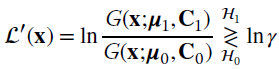
and ![]() . It can be shown that the NP lemma applies as covariances are known, and the log‐LRT (apart from additive terms that are accounted for in the threshold γ)
. It can be shown that the NP lemma applies as covariances are known, and the log‐LRT (apart from additive terms that are accounted for in the threshold γ)
is a quadratic form with
The factorization ![]() from
from ![]() (and
(and ![]() ) allows the log‐LRT to be rewritten as
) allows the log‐LRT to be rewritten as
with ![]() (pre‐whiten of x) and
(pre‐whiten of x) and ![]() . The distribution of the log‐LRT is a chi‐square pdf, and the NP lemma for a given γ needs to detail the pdf of
. The distribution of the log‐LRT is a chi‐square pdf, and the NP lemma for a given γ needs to detail the pdf of ![]() (x) under
(x) under ![]() 0 and
0 and ![]() 1 (see Section 4.14 of [7] ).
1 (see Section 4.14 of [7] ).
23.4 Bayesian Classification
The case where the probabilistic structure of the underlying classes is known perfectly is an excellent theoretical reference to move on to the Bayesian classifiers characterized by the a‐priori probabilities on each class. Let ![]() classes, the a‐priori information on classes is in form of probabilities p(
classes, the a‐priori information on classes is in form of probabilities p(![]() 1) and p(
1) and p(![]() 0), with known
0), with known ![]() and
and ![]() . The misclassification error is when
. The misclassification error is when ![]() for class
for class ![]() 1 and vice‐versa, and the probability is
1 and vice‐versa, and the probability is
Minimization of Pr(error) defines the optimal decision region with minimum misclassification probability, which is minimized when assigning each value x to the class ![]() k that has the largest a‐posteriori probability
k that has the largest a‐posteriori probability ![]() . Class
. Class ![]() 1 is assigned when
1 is assigned when
but according to Bayes’ rule it can be rewritten in terms of likelihood ratio for the two alternative classes
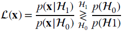
where the threshold depends on the a‐priori probabilities. In the case where ![]()
![]() , the decision in favor of class
, the decision in favor of class ![]() 1 is when
1 is when ![]() as in Section 23.3.2. For example, the binary classification for Gaussian distributions (Section 23.2.2) that minimizes the Pr(error) yields the decision rule
as in Section 23.3.2. For example, the binary classification for Gaussian distributions (Section 23.2.2) that minimizes the Pr(error) yields the decision rule

Again, the decision boundary characteristics do not change between linear and quadratic.
For K classes, the misclassification error is
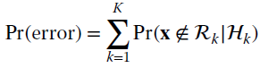
and it needs to compare x with ![]() decision regions (e.g., it could be too complex). Alternatively, one evaluates the probability of correct classification given by
decision regions (e.g., it could be too complex). Alternatively, one evaluates the probability of correct classification given by

which is maximized when choosing for x the class ![]() k that has the largest a‐posteriori probability
k that has the largest a‐posteriori probability ![]() compared to all the others.
compared to all the others.
23.4.1 To Classify or Not to Classify?
Decisions should be avoided when too risky. One would feel more confident to decide in favor of ![]() k if
k if ![]() and all the others are
and all the others are ![]() for
for ![]() . When all the a‐posteriori probabilities are comparable (i.e., for K classes,
. When all the a‐posteriori probabilities are comparable (i.e., for K classes, ![]() , still
, still ![]() ), any decision is too risky and the decision could be affected by errors (e.g., due to the inappropriate a‐priori probabilities), and misclassification error occurs. The way out of this is to introduce the reject class, which express doubt on a decision. A simple approach for a binary decision is to add an interval
), any decision is too risky and the decision could be affected by errors (e.g., due to the inappropriate a‐priori probabilities), and misclassification error occurs. The way out of this is to introduce the reject class, which express doubt on a decision. A simple approach for a binary decision is to add an interval ![]() to the decision such that the a‐posteriori probabilities for the decision become
to the decision such that the a‐posteriori probabilities for the decision become
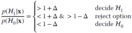
Alternatively, the reject option can be introduced by setting a minimum threshold on the a‐posteriori probabilities for classifying, say pt, such that even if one would decide for ![]() k as
k as ![]() , this choice is rejected if
, this choice is rejected if ![]() . The threshold pt controls the fraction to be rejected: all are rejected if
. The threshold pt controls the fraction to be rejected: all are rejected if ![]() , all are classified if
, all are classified if ![]() , and for K classes the threshold is approx.
, and for K classes the threshold is approx. ![]() . When the fraction of rejections is too large, further experiments or training are likely to be necessary.
. When the fraction of rejections is too large, further experiments or training are likely to be necessary.
23.4.2 Bayes Risk
The error probability (23.8) could be inappropriate in some contexts where errors ![]() and
and ![]() are perceived differently. To exemplify, consider medical screening for early cancer diagnosis to compare the presence of a cancer (class
are perceived differently. To exemplify, consider medical screening for early cancer diagnosis to compare the presence of a cancer (class ![]() 1) compared to being healthy (class
1) compared to being healthy (class ![]() 0). The incorrect diagnosis of cancer when a patient is healthy (
0). The incorrect diagnosis of cancer when a patient is healthy (![]() ) induces some further investigations and psychological discomfort; the wrong diagnosis of lack of any pathology when the cancer is already in an advanced state (
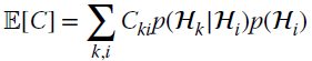
) induces some further investigations and psychological discomfort; the wrong diagnosis of lack of any pathology when the cancer is already in an advanced state (![]() ) delays the cure and increases secondary risks. The two errors have different impact that can be accounted for with a different cost function (sometime referred as loss function) Cki that is the cost of choosing
) delays the cure and increases secondary risks. The two errors have different impact that can be accounted for with a different cost function (sometime referred as loss function) Cki that is the cost of choosing ![]() k when
k when ![]() i is the true class. For cancer diagnosis,
i is the true class. For cancer diagnosis, ![]() . The optimum classification is the one that minimizes the average cost
. The optimum classification is the one that minimizes the average cost ![]() , defined from the expectation and called Bayes risk:
, defined from the expectation and called Bayes risk:
Usually ![]() , but in any case it is a common choice not to apply any cost to correct decisions hence
, but in any case it is a common choice not to apply any cost to correct decisions hence ![]() . The Bayes risk for
. The Bayes risk for ![]() is
is
(recalling that ![]() ). The choice of the decision region to minimize (23.10) does not depend on its first term, but rather on the remaining two terms that can be rearranged as
). The choice of the decision region to minimize (23.10) does not depend on its first term, but rather on the remaining two terms that can be rearranged as
These resemble the minimization of the error probability (23.8) after correcting the a‐priori probabilities as ![]() and
and ![]() , for a normalization factor α of probabilities. The LRT is
, for a normalization factor α of probabilities. The LRT is
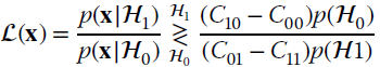
and the threshold is modified to take into account the cost functions applied to the decisions (for ![]() and
and ![]() it coincides with the threshold (23.9)).
it coincides with the threshold (23.9)).
23.5 Pattern Recognition and Machine Learning
Classification when the problem is complex (K large) and data is large (N large) should use a preliminary training stage to define by samples the decision regions (or their boundaries), and classification is by recognizing the “similarity” with one of the patterns used during the training. The simplest classifier for binary classes is a linear decision boundary, which is shown in Section 23.2.2 to be optimum when Gaussian distributions of the two classes have the same covariances. The simplest pattern recognition method is the perceptron algorithm, which is a supervised learning algorithm for the linear binary classifier developed in the early 60s, and is celebrated as the first artificial neural network classifier. Machine learning methods have evolved a great deal since then, and the support vector machine (SVM) is one of the most popular ones today. An excellent overview of the methods is by Bishop [136].
23.5.1 Linear Discriminant
The linear classifier function between two classes can be stated as follows:
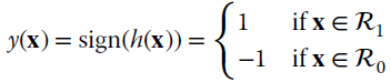
where
is the linear discriminant function that depends on (a, b); the decision boundary ![]() describes a hyperplane in N‐dimensional space. To illustrate the geometrical meanings, Figure 23.6 shows the case of
describes a hyperplane in N‐dimensional space. To illustrate the geometrical meanings, Figure 23.6 shows the case of ![]() . The orthogonality condition
. The orthogonality condition ![]() states that any value of x along the boundary is orthogonal to the unit‐norm vector
states that any value of x along the boundary is orthogonal to the unit‐norm vector ![]() . The distance of the (hyper)plane from the origin is defined by b by taking the point xo perpendicular to the origin, hence
. The distance of the (hyper)plane from the origin is defined by b by taking the point xo perpendicular to the origin, hence

Figure 23.6 Linear discriminant for  .
.
The signed distance of any point from the boundary is
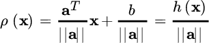
and this can be easily shown once decomposed ![]() into its value along the boundary xp (projection of x onto the hyperplane) and its distance
into its value along the boundary xp (projection of x onto the hyperplane) and its distance ![]() .
.
Extending to K classes, the linear discriminant can follow the same rules as in Section 23.3.2 by defining K linear discriminants such as for the kth class
and one decides in favor of ![]() k when
k when
This is called a one‐versus‐one classifier. This decision rule reflects the notion of distance from each hyperplane, and one chooses for the largest. The decision boundary ![]() can be found by solving
can be found by solving
Notice that the decision regions defined from the linear discriminants are simply connected and convex (i.e., any two points in ![]() k are connected by a line in
k are connected by a line in ![]() k). A one‐versus‐one classifier involves
k). A one‐versus‐one classifier involves ![]() comparisons, and one could find that there is not only one class that prevails. This creates an ambiguity that is solved by majority vote: the class that has the greatest consensus wins.
comparisons, and one could find that there is not only one class that prevails. This creates an ambiguity that is solved by majority vote: the class that has the greatest consensus wins.
23.5.2 Least Squares Classification
Learning the parameter vectors (ak, bk) of linear classifiers is the first step in supervised pattern recognition. The LS method fits hyperplanes to the set of training vectors. Let (xℓ, tℓ) be the ℓth training vector and the coding vector pair for a class ![]() k; this means that the coding vector encodes the information on the class by assigning the kth entry
k; this means that the coding vector encodes the information on the class by assigning the kth entry ![]() and
and ![]() for all the others
for all the others ![]() . The K linear discriminants are grouped as
. The K linear discriminants are grouped as
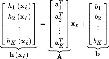
The classifiers can be found by minimizing the LS from all coding vectors tℓ:

over all the training set ![]() . The decision functions
. The decision functions ![]() derived from the LS minimization are a combination of trainings
derived from the LS minimization are a combination of trainings ![]() , and this is quite typical of pattern recognition methods.
, and this is quite typical of pattern recognition methods.
After the learning stage, one can recognize the pattern (also called class prediction) by evaluating the metric for the current x
and choosing the largest one. Even if the entries of training tℓ take values {0, 1} and resemble the classification probabilities, the discriminant ĥ(x) for any x is not guaranteed to be in the range [0, 1]. Furthermore, LS implicitly assumes that the distribution of each class is Gaussian, and the LS coincides with the MLE in this case and is sub‐optimal otherwise. The target coding scheme can be tailored differently from the choice adopted here—see [136].
23.5.3 Support Vectors Principle
Linear classifiers can be designed based on the concept of margin, and this is illustrated here for the binary case. Considering a training set
where binary valued
encodes the two classes; the linear classifier is (a, b) such that the training classes are linearly separable:

This is equivalent to rewriting the trainings into
where the equality is for the margins illustrated in Figure 23.7. The optimal hyperplane is from signed ρ(x) for the optimal margins such that the relative distance
is maximized. The maximum value is for the margins corresponding to the support vectors
xℓ such that ![]() , and the optimal margin is
, and the optimal margin is
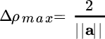

Figure 23.7 Support vectors and margins from training data.
The optimal hyperplane is the one that minimizes the norm ![]() (or equivalently, maximizes the margin) subject to the constraint (23.11), and this yields the maximum margin linear classifier.
(or equivalently, maximizes the margin) subject to the constraint (23.11), and this yields the maximum margin linear classifier.
This statement can be proved analytically, and the optimization is written using the Lagrange multiplier [137] :
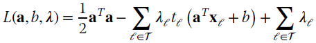
with ![]() . Taking the gradients wrt a yields:
. Taking the gradients wrt a yields:
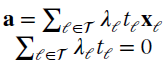
which implies that the optimal hyperplane is a linear combination of the training vectors, and the classifier is
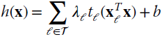
in terms of weighted linear combination of the inner products with all the trainings. The SVM solves the optimization by reformulating the Lagrangian (23.12) in terms of the equivalent representation:
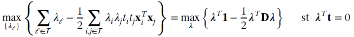
where ![]() ,
, ![]() , and
, and ![]() contains all the inner products of the training vectors arranged in a matrix. This reduces to a constrained optimization for a quadratic form in λ, with the additional constraint
contains all the inner products of the training vectors arranged in a matrix. This reduces to a constrained optimization for a quadratic form in λ, with the additional constraint ![]() . This representation proves that the constraint
. This representation proves that the constraint ![]() is guaranteed by an equality only for
is guaranteed by an equality only for ![]() where
where ![]() is the constraint (23.11), and these are the support vectors. This means that the classifier (23.13) depends only on the support vectors, as for all others,
is the constraint (23.11), and these are the support vectors. This means that the classifier (23.13) depends only on the support vectors, as for all others, ![]() .
.
The optimization (23.14) is quadratic and can be iterative. The size of the inner products matrix D is ![]() ; the memory occupancy scales with
; the memory occupancy scales with ![]() and this could be very challenging when the training set is large. Numerical methods are adapted to solve this problem—such as those based on the decomposition of the optimization problem on set λ into two disjoint sets called active λA and inactive λN part [138]. The optimality condition holds for λA when setting λN=0, and the active part should include the support vector (with
and this could be very challenging when the training set is large. Numerical methods are adapted to solve this problem—such as those based on the decomposition of the optimization problem on set λ into two disjoint sets called active λA and inactive λN part [138]. The optimality condition holds for λA when setting λN=0, and the active part should include the support vector (with ![]() ). The active set is not known but it should be chosen arbitrarily and refined iteratively by solving at every iteration for the sub‐problem that is related to the active part only.
). The active set is not known but it should be chosen arbitrarily and refined iteratively by solving at every iteration for the sub‐problem that is related to the active part only.
The SVM plane (or surface) is based on a distinguishable, reliable, and noise‐free training set. However, in practice the training could be unreliable, or even maliciously manipulated to affect the classification error. This calls for a robust approach to SVM that modifies the constraint on trainings (23.11) by introducing some regularization terms (see e.g., [139] [140] ).
Remark: Classification surfaces are not only planar, but in general can be arbitrary to minimize the classification error and their shapes depend on the problem at hand, and in turn their (unknown) pdfs. Non‐linear SVM is application‐specific and it needs some skill for its practical usage for pattern‐recognition. The key conceptual point is that the arrangement ![]() contains the training data only as an inner product. One can apply a non‐linear transformation ϕ(.) that maps xℓ onto another space ϕ(xℓ) where training vectors can be better separated by hyperplanes, and one can define the corresponding inner products ϕT(xi)ϕ(xj), called kernels, to produce a non‐linear SVM. The topic is broad and problem‐dependent, and the design of ϕ(.) needs experience. A discussion is beyond the scope here, and the reader is referred to [136] [140].
contains the training data only as an inner product. One can apply a non‐linear transformation ϕ(.) that maps xℓ onto another space ϕ(xℓ) where training vectors can be better separated by hyperplanes, and one can define the corresponding inner products ϕT(xi)ϕ(xj), called kernels, to produce a non‐linear SVM. The topic is broad and problem‐dependent, and the design of ϕ(.) needs experience. A discussion is beyond the scope here, and the reader is referred to [136] [140].
23.6 Clustering
Originally clustering was considered as a signal processing method for vector quantization (or data compression) where it is relevant to encode each N‐dimensional vector x by using K fixed vectors (codevectors) μ1, μ2, …, μK each of dimension N. This is based on a set of encoding regions ![]() 1,
1, ![]() 2, …,
2, …, ![]() K, possibly disjoint (
K, possibly disjoint (![]() ), associated to each codevector (μk is uniquely associated to
), associated to each codevector (μk is uniquely associated to ![]() k) such that when any vector x is in the encoding region
k) such that when any vector x is in the encoding region ![]() k, then its approximation is μk and this is denoted as
k, then its approximation is μk and this is denoted as
Representation of x by the K codevectors is affected by a distortion that is ![]() , and the mean square distortion is
, and the mean square distortion is
considering the pdf of x (or its sample value if unavailable, or the training set). Design of the encoding regions (Figure 23.8) is to minimize the mean square distortion D, and this in turn provides a reduced‐complexity representation of any x by indexing the corresponding codevector Q(x) that, being limited to K values, can be represented at most by a limited set of log2K binary values. Distortion D is monotonic decreasing in the number of codevectors K, but the codevectors should be properly chosen according to the pdf p(x) as it is essentially a parsimonious (but distorted) representation of x.
Figure 23.8 Clustering methods: K‐means (left) and EM (right) vs. iterations.
23.6.1 K‐Means Clustering
K‐means is the simplest clustering method, which makes an iterative assignment of the L samples x1, x2, …, xL to a predefined number of clusters K. One starts from a initial set of values ![]() that represent the cluster centroids. Each sample xℓ is assigned to the closest centroid, and after all samples are assigned, the new centroids are recomputed. It is convenient to use the binary variables
that represent the cluster centroids. Each sample xℓ is assigned to the closest centroid, and after all samples are assigned, the new centroids are recomputed. It is convenient to use the binary variables ![]() to indicate which cluster the ℓth sample xℓ belongs to:
to indicate which cluster the ℓth sample xℓ belongs to: ![]() if xℓ is assigned to the kth cluster, and
if xℓ is assigned to the kth cluster, and ![]() for
for ![]() . The mean square distortion
. The mean square distortion

dependsn the choice of cluster centroids, which are obtained iteratively. K‐means clustering in pseudo‐code is (see also Figure 23.8):
Initialize by ![]()
- for
 , assign
  if
if 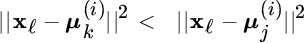 for
for  :
:  ; end
; end - recalculate the position of the centroids:

- iterate to 1) until the centroids do not change vs. iterations (
 for
for  ).
).
Even if the K‐means algorithm converges, the convergence clustering depends on the initial choice of centroids ![]() . There is no guarantee that the convergence really minimizes the mean square distortion D, and to avoid convergence to bad conditions one can initialize over a random set
. There is no guarantee that the convergence really minimizes the mean square distortion D, and to avoid convergence to bad conditions one can initialize over a random set ![]() and choose the best clustering based on its smallest distortion D. Notice that for a random initialization, there could be cluster centroids that have no samples assigned, and do not update. Further, the number of clusters K can be a free parameter, and clusters can be split or merge to solve for some critical settings. A good reference is Chapter 8 of [142].
and choose the best clustering based on its smallest distortion D. Notice that for a random initialization, there could be cluster centroids that have no samples assigned, and do not update. Further, the number of clusters K can be a free parameter, and clusters can be split or merge to solve for some critical settings. A good reference is Chapter 8 of [142].
23.6.2 EM Clustering
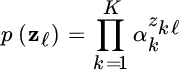
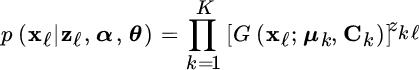
Let the data set x1, x2, …, xL be a sample set of the pdf p(x) that is from the Gaussian mixture model (Section 11.6.3):

where ![]() ) are the moments characterizing the N‐dimensional Gaussian pdf of the kth class with parameters θk, and
) are the moments characterizing the N‐dimensional Gaussian pdf of the kth class with parameters θk, and ![]() is the mixing proportions (or coefficients) that are constrained to
is the mixing proportions (or coefficients) that are constrained to

In expectation maximization (EM) clustering, the complete set is obtained by augmenting each sample value xℓ by the corresponding missing data that describe the class of each sample to complete the data set. In detail, to complete the data there is a new set of latent variables
z1, z2, …, zL that describe which class each sample x1, x2, …, xL belongs to by a binary class‐indexing variable ![]() , where
, where ![]() means that xℓ belongs to kth class. The marginal probability of zℓ is dependent on the mixing proportions as
means that xℓ belongs to kth class. The marginal probability of zℓ is dependent on the mixing proportions as
and the conditional pdf is
The complete data is ![]() and the EM method contains the E‐step to estimate iteratively the latent variables {z1, z2, …, zL} and the M‐step for the mixture parameters α, θ. Since the joint probability is
and the EM method contains the E‐step to estimate iteratively the latent variables {z1, z2, …, zL} and the M‐step for the mixture parameters α, θ. Since the joint probability is
(recall that ![]() and
and ![]() ), the conditional probability
), the conditional probability
is the product of all the pdfs depending on which rv in zℓ is active, and the joint pdf is

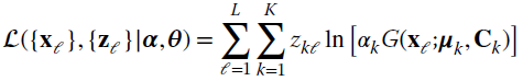
The likelihood of the complete data is:

and the log‐likelihood is
The E‐step is to estimate the latent variables zkℓ as ![]() (iteration number is omitted to avoid a cluttered notation). From Bayes, one gets the probability of xℓ belonging to the kth class from the property of the mixture [45,143] :
(iteration number is omitted to avoid a cluttered notation). From Bayes, one gets the probability of xℓ belonging to the kth class from the property of the mixture [45,143] :

which yields the estimate of the latent variables based on the current mixture parameters α, θ.
The M‐step estimates the means and covariances of the new Gaussian mixture based on the latent variables {ẑkℓ} by maximizing the log‐likelihood (23.16). The MLE of θ can be obtained from the log‐likelihood function

Setting the gradients to zero (see Section 1.4 for gradients)

one obtains the update equations
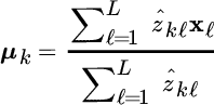
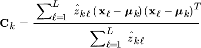
which are a weighted average by the a‐posteriori probability ![]() for each sample xℓ and the kth class.
for each sample xℓ and the kth class.
The mixing set α can be obtained by optimizing the log‐likelihood (23.17) wrt α, constrained by sum (23.15) using the Lagrange multiplier (Section 1.8). The mixing coefficients

are be used for the next iterations.
The EM can be interpreted as follows. At each iteration, the a‐posteriori probabilities ẑ1ℓ, ẑ2ℓ, …, ẑKℓ on classes of each sample xℓ are evaluated based on the mixture parameters previously computed. Using these probabilities, the means and covariances for each class are re‐estimated (23.18, 23.19) depending on the class‐assignment probabilities ẑ1ℓ, ẑ2ℓ, …, ẑKℓ. The corresponding mixing probabilities are re‐calculated accordingly as in (23.20). Notice that re‐estimation of moments (23.18, 23.19) is weighted by the a‐posteriori probabilities ẑk1, ẑk2, …, ẑkL and if the class is empty (i.e., ẑkℓ is mostly small for all samples x1, x2, …, xL, or equivalently αk from (23.20) is very small), the EM update can be unstable.
At convergence, the estimate of the latent variables ẑkℓ gives the a‐posteriori probability for each data xℓ and the kth cluster. EM clustering can be interpreted as an assignment to each cluster based on the a‐posteriori probability. For comparison, K‐means clustering makes a sharp assignment of each sample to the cluster, while the EM method makes a soft assignment based on the a‐posteriori probabilities. EM clustering degenerates to K‐means for the choice of symmetric Gaussians with ![]() , and σ2 small and fixed, the a‐posteriori clustering becomes
, and σ2 small and fixed, the a‐posteriori clustering becomes

which for small enough σ2 has ![]() as
as ![]() for
for ![]() .
.
Note that EM clustering might converge to a local optimum that depends on the initial conditions and the choice of the number of clusters K. Initialization could be non‐informative with a random starting point: ![]() . The number of clusters K should be set and kept fixed over the iterations. Clusters can be annihilated during iterations when not supported by data, one component of the mixture is too weak, and one value αk is excessively small (i.e., since αk is the probability that one sample belongs to the kth class, it is clear that when
. The number of clusters K should be set and kept fixed over the iterations. Clusters can be annihilated during iterations when not supported by data, one component of the mixture is too weak, and one value αk is excessively small (i.e., since αk is the probability that one sample belongs to the kth class, it is clear that when ![]() there are not enough samples to update the classes). This can be achieved by setting their mixing proportion to zero [143].
there are not enough samples to update the classes). This can be achieved by setting their mixing proportion to zero [143].