
20
Multichannel Time of Delay Estimation
Time of delay (ToD) estimation is a very common problem in many applications that employ wavefield propagation such as radar, remote sensing, and geophysics (Section 18.5) where the information of interest is mapped onto ToDs. Features of the wavefields call for measurement redundancy from a multichannel system where there are ![]() signals that are collected as s1(t), s2(t), …, sM(t), and this leads to massive volumes of data for estimating the ToD metric. The uniform linear array in Chapter 19 represents a special case of a multichannel system where the source(s) is narrowband and the only parameter(s) that can be estimated is the DoA(s). Here the narrowband constraint is removed while still preserving the multidimensionality of the signals in order to have the needed redundancy for estimating the ToD variation vs. measuring channels (e.g., sensors) with known geometrical positions.
signals that are collected as s1(t), s2(t), …, sM(t), and this leads to massive volumes of data for estimating the ToD metric. The uniform linear array in Chapter 19 represents a special case of a multichannel system where the source(s) is narrowband and the only parameter(s) that can be estimated is the DoA(s). Here the narrowband constraint is removed while still preserving the multidimensionality of the signals in order to have the needed redundancy for estimating the ToD variation vs. measuring channels (e.g., sensors) with known geometrical positions.
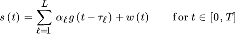
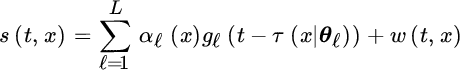
The multichannel concept is illustrated in Figure 20.1 from seismic exploration (see Section 18.5 or [82] ): the wavefield generated at the surface propagates in the subsurface and is backscattered at depth discontinuities, and measured with sensors at the surface. The wavefield is collected by a regularly spaced 2D array of sensors to give the measured wavefields s(x, y, t) in space (x, y) and time t in the figure. Note that in Figure 20.1 the 3D volume s(x, y, t) of 1.3 km ![]() 10 km is sliced along planes to illustrate by gray‐scale images the complex behavior of multiple backscattered wavefronts, and the corresponding ToD discontinuities of wavefronts due to subsurface faults. Multichannel ToD estimation refers to the estimation of the ensemble of ToDs pertaining to the same wavefront represented by a 2D surface τℓ(x, y) that models the ℓ th delayed wavefront characterized by a spatial continuity.1 The measured wavefield can be modeled as a superposition of echoes (for any position x, y)
10 km is sliced along planes to illustrate by gray‐scale images the complex behavior of multiple backscattered wavefronts, and the corresponding ToD discontinuities of wavefronts due to subsurface faults. Multichannel ToD estimation refers to the estimation of the ensemble of ToDs pertaining to the same wavefront represented by a 2D surface τℓ(x, y) that models the ℓ th delayed wavefront characterized by a spatial continuity.1 The measured wavefield can be modeled as a superposition of echoes (for any position x, y)

where the amplitudes αℓ(x, y) and ToDs τℓ(x, y) are wavefront and sensor dependent, and g(t) is the excitation waveform.

Figure 20.1 Multichannel measurements for subsurface imaging.
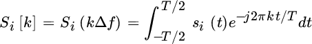
The ToD from multiple measurements is by chaining multiple distinct sensors. A radar system can be interpreted as a multichannel model when estimating the ToD variation vs. the scanning time when the target(s) move(s) from one time‐scan to another, or the radar antenna moves for a still target (e.g., satellite remote sensing of the earth). Regardless of the origin of the multiplicity of measurements, the most general model for multichannel ToD for the i th measurement (Figure 20.2):

is the superposition of L echoes each with waveform gℓ(t), amplitude αℓ,i, and ToD τℓ,i as sketched below in gray‐intensity plot with superimposed the trajectory of the ToD {τℓ,i} vs. the sensor’s position (black‐line). ToD estimation refers to the estimation of the delays  for a specific measurement, and the amplitudes
  could be nuisance parameters. However, when considering a collection of measurements s1(t), s2(t), …, sM(t), multichannel ToD estimation refers to the estimation of the ToD profile for the ℓ th wavefront (i.e., a collection of ToD vs. sensor):
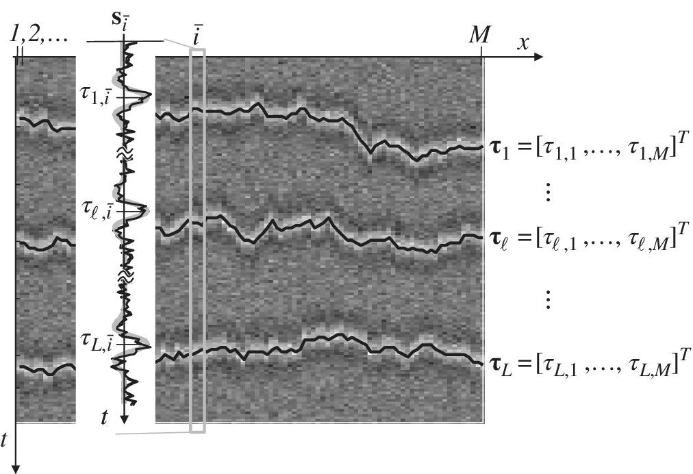
Figure 20.2 Multichannel ToD model.
Parametric wavefront: Estimation of ToDs of the wavefront(s) as a collection of the corresponding delays. The wavefront can be parameterized by a set of wavefront‐dependent geometrical and kinematical shape parameters θℓ (e.g., sensors position, sources position, and propagation velocity) as illustrated in Section 18.5, so that the ToD dependency is
To exemplify, one can use a linear model for the ToDs ![]() so that the wavefront can be estimated by estimating the two parameters
so that the wavefront can be estimated by estimating the two parameters ![]() instead. The estimation of the shape parameters from a set of redundant (
instead. The estimation of the shape parameters from a set of redundant (![]() ) measurements has the benefit of tailoring ToD methods to estimate the sequence of ToDs vs. a measurement index as in Figure 20.2. Applications are broad and various such as wavefield based remote sensing, radar, and ToD tracking using Bayesian estimation methods (Section 13.1). To illustrate, when two flying airplanes cross, one needs to keep the association between the radar’s ToDs and the true target positions as part of the array processing (Chapter 19). Only the basics are illustrated in this chapter, leaving the full discussion to application‐related specialized publications.
) measurements has the benefit of tailoring ToD methods to estimate the sequence of ToDs vs. a measurement index as in Figure 20.2. Applications are broad and various such as wavefield based remote sensing, radar, and ToD tracking using Bayesian estimation methods (Section 13.1). To illustrate, when two flying airplanes cross, one needs to keep the association between the radar’s ToDs and the true target positions as part of the array processing (Chapter 19). Only the basics are illustrated in this chapter, leaving the full discussion to application‐related specialized publications.
Active vs. passive sensing systems: The waveforms g1(t), g2(t), …, gL(t) can be different to one another and dependent on the sources, which are not necessarily known. A radar/sonar system (Section 5.6) or seismic exploration (Section 18.5) are considered as active systems as the waveforms are generated by a controlled source and all waveforms are identical (![]() ), possibly designed to maximize the effective bandwidth (Section 9.4) and thus the resolution for multiple echoes. In contrast to active systems, in passive systems the waveforms are different from one another, modeled as stochastic processes characterized in terms of PSD. An example of a passive system is the acoustic signal in an concert hall, which is the superposition of signals from many musical instruments. The scenario is complex, and Table 20.1 offers a (limited and essential) taxonomy of the methods and summarizes those discussed in this chapter.
), possibly designed to maximize the effective bandwidth (Section 9.4) and thus the resolution for multiple echoes. In contrast to active systems, in passive systems the waveforms are different from one another, modeled as stochastic processes characterized in terms of PSD. An example of a passive system is the acoustic signal in an concert hall, which is the superposition of signals from many musical instruments. The scenario is complex, and Table 20.1 offers a (limited and essential) taxonomy of the methods and summarizes those discussed in this chapter.
Table 20.1 Taxonomy of ToD methods.
| # sensors (M) | # ToD (L) | gℓ(t) | ToD estimation method |
| 1 | 1 | known | MLE (Section 9.4) |
| 2 | 1 | not‐known | Difference of ToD (DToD) (Section 20.3) |
| 1 | MLE for multiple echoes (Section 20.2) | ||
| 1 | known | MLE/Shape parameters estimation (Section 20.5) | |
| 1 | non‐known | Shape parameters estimation (Section 20.6) | |
| known | Multi‐target ToD tracking [92] |
20.1 Model Definition for ToD
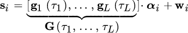
The ToD problem for multiple echoes is continuous‐time estimation that must be modified to accommodate discrete‐time data. The time‐sampled signals are modeled as in Section 5.6:

where ![]() is the column that orders the ℓ th delayed waveform sampled in {t1, t2, …, tN}, and noise
is the column that orders the ℓ th delayed waveform sampled in {t1, t2, …, tN}, and noise ![]() . Dependence of the ToDs is non‐linear and it is useful to exploit the quadratic dependency on the amplitudes αi in the ML method (Section 7.2.2):
. Dependence of the ToDs is non‐linear and it is useful to exploit the quadratic dependency on the amplitudes αi in the ML method (Section 7.2.2):
The MLE follows from the optimization
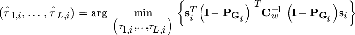
where ![]() . In the case of a white Gaussian noise process (
. In the case of a white Gaussian noise process (![]() ), the optimization for ML ToD estimation reduces to the maximization of the metric
), the optimization for ML ToD estimation reduces to the maximization of the metric

where the projection matrix ![]() imbeds into the matrix
imbeds into the matrix ![]() all the products
all the products ![]() that account for the mutual interference of the different waveforms. A special case is when the amplitudes are changing, but the delays (τ1, …, τL) are not:
that account for the mutual interference of the different waveforms. A special case is when the amplitudes are changing, but the delays (τ1, …, τL) are not:
This model reduces to the MLE in Section 7.2.3 and gives
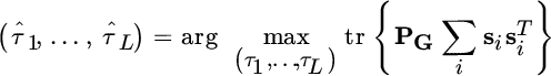
The influence of noise and amplitude fluctuations is mitigated by the averaging of the outer products ![]() .
.
Recall (Section 9.4) that for ![]() and
and ![]() , the MLE depends on the maximization of
, the MLE depends on the maximization of
that is the cross‐correlation between the samples of {s[n]} and the continuous‐time waveform g(t) arbitrarily shifted (by τ) and regularly sampled by the same sampling interval Δt of ![]() . However, if the waveform is only available as sampled g[k] at sampling interval Δt, the cross‐correlation (20.1) can be evaluated over a coarse sample‐grid (Section 10.3), or it requires that the discrete‐time waveform is arbitrarily shifted by a non‐integer and arbitrary delay τ, and this can be obtained by interpolation and resampling (Appendix B).
. However, if the waveform is only available as sampled g[k] at sampling interval Δt, the cross‐correlation (20.1) can be evaluated over a coarse sample‐grid (Section 10.3), or it requires that the discrete‐time waveform is arbitrarily shifted by a non‐integer and arbitrary delay τ, and this can be obtained by interpolation and resampling (Appendix B).
20.2 High Resolution Method for ToD (L=1)
Let the model be
with known waveform g(t). The MLE of the ToDs
for ![]() is a multidimensional search over L‐dimensions (see Section 9.4 for
is a multidimensional search over L‐dimensions (see Section 9.4 for ![]() ) that might be affected by many local maxima, and the ToD estimate could be affected by large errors when waveforms are severely overlapped. High‐resolution methods adapted from the frequency estimation in Chapter 16 have been proposed in the literature and are based on some simple similarities reviewed below.
) that might be affected by many local maxima, and the ToD estimate could be affected by large errors when waveforms are severely overlapped. High‐resolution methods adapted from the frequency estimation in Chapter 16 have been proposed in the literature and are based on some simple similarities reviewed below.
20.2.1 ToD in the Fourier Transformed Domain
The model after the Fourier transform of the data (20.2) is

Since the waveform is known, its Fourier transform G(ω) is known and the observation can be judiciously deterministically deconvolved (i.e., S(ω) is divided by G(ω) except when ![]() ) so that after deconvolution:
) so that after deconvolution:
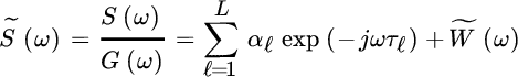
This model resembles the frequency estimation in additive Gaussian noise, where the ToD τℓ induces a linear phase‐variation vs. frequency, rather than a linear phase‐variation vs. time as in the frequency estimation model (Chapter 16).
Based on this conceptual similarity, the discrete‐time model can be re‐designed using the Discrete Fourier transform (Section 5.2.2) over N samples ![]() to reduce the model (20.2) to (20.3):
to reduce the model (20.2) to (20.3):

where the ℓ th ToD τℓ makes the phase change linearly over the sample index k
behaving similarly to a frequency that depends on the sampling interval Δt. If considering multiple independent observations with randomly varying amplitudes  as in the model in Section 20.1, the ToD estimation from the estimate of
 ![]() coincides with frequency estimation, and the high‐resolution methods in Chapter 16 can be used with excellent results.
coincides with frequency estimation, and the high‐resolution methods in Chapter 16 can be used with excellent results.
In many practical applications, there is only one observation (![]() ) and the model (20.4) can be represented in compact notation (N is even):
) and the model (20.4) can be represented in compact notation (N is even):
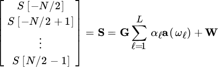
where
and
contains the DFT of the waveform ![]() . The estimation of multiple ToDs follows from LS optimization of the cost function:
. The estimation of multiple ToDs follows from LS optimization of the cost function:
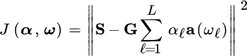
The LS method coincides with MLE when the noise samples W[k] are Gaussian and mutually uncorrelated. Since the DFT of Gaussian white process w(nΔt) leaves the samples W[k] to be uncorrelated due to the unitary transformation property of DFT, the minimization of J(α, ω) coincides with the MLE.
One numerical method to optimize J(α, ω) is by the weighted Fourier transform RELAXation (W‐RELAX) iterative method that resembles the iterative steps of EM (Section 11.6), where at every iteration the estimated waveforms are stripped from the observations for estimation of one single parameter [95]. In detail, let the set ![]() be known as estimated at previous steps, after stripping these waveforms
be known as estimated at previous steps, after stripping these waveforms

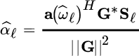
one can use a local metric for the ℓ th ToD and amplitude
As usual, this is quadratic wrt αℓ and it can be easily solved for the frequency ωℓ (i.e., the ℓ th ToD)
and the amplitude follows once ![]() has been estimated as
has been estimated as
Iterations are carried out until some degree of convergence is reached. Improved and faster convergence is achieved by adopting IQML (Section 16.3.1) in place of the iterations of W‐RELAX.
The methods above can be considered extensions of statistical methods discussed so far, but some practical remarks are necessary:
- Any frequency domain method needs to pay attention to the shape of G(ω), or the equivalent DFT samples G[k]. In definitions, the range of G should be limited to those values that are meaningfully larger than zero to avoid instabilities in convergence. However, restricting the range for ω reduces ToD accuracy considerably as it is dominated by higher frequencies in the computation of the effective bandwidth (Section 9.4). Similar reasoning holds when performing deterministic deconvolution if using other high‐resolution methods, as the deconvolution 1/G(ω) can be stabilized by conditioning that is adding a constant term to avoid singularities such as
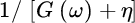 , where η is a small fraction of max{|G(ω)|}.
 - Conditioning and accuracy are closely related. In some cases in iterative estimates it is better to avoid temporary ToD estimates getting too close one another: one can set a ToD threshold, say Δω, that depends on the waveforms. In this case, the estimates from the iterative methods above that are too close, say
 and
and  with
with  and
and  , are replaced by
 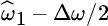 and
and  to improve convergence and accuracy.
20.2.2 CRB and Resolution
As usual, the CRB is a powerful analytic tool to establish the accuracy bound. In the case of ToD, the performance depends on the waveforms and their spectral content as detailed in Section 9.4 for ![]() ToDs. When considering multiple delays, the CRB depends on the FIM entries, which for white Gaussian noise with power spectral density N0/2 can be evaluated in closed form as:
ToDs. When considering multiple delays, the CRB depends on the FIM entries, which for white Gaussian noise with power spectral density N0/2 can be evaluated in closed form as:
Recall that the choice of the waveform is a powerful degree of freedom in system design to control ToD accuracy when handling multiple and interfering echoes. Choice of waveform and range can satisfy ![]() and
and ![]() so that two (or more) ToDs are decoupled and the correlation‐based ML estimator can be applied iteratively on each echo. In all the other contexts when
so that two (or more) ToDs are decoupled and the correlation‐based ML estimator can be applied iteratively on each echo. In all the other contexts when ![]() and/or
and/or ![]() , the CRB for multiple echoes is larger than the CRB for one isolated echo due to the interaction of the waveforms, and it can be made dependent on their mutual interaction as illustrated in the simple example in Section 9.4 with
, the CRB for multiple echoes is larger than the CRB for one isolated echo due to the interaction of the waveforms, and it can be made dependent on their mutual interaction as illustrated in the simple example in Section 9.4 with ![]() .
.
With multiple echoes, resolution is the capability to distinguish all the echoes by their different ToDs. Let a measurement be of ![]() echoes in τ1 and τ2 (
echoes in τ1 and τ2 (![]() ) with the same waveform; it is obvious that when the two ToDs are very close, if not coincident, the two waveforms coincide and are misinterpreted as one echo, possibly with a small waveform distortion that might be interpreted as noise. Most of the tools to evaluate the performance in this situation are by numerical experiments using common sense and experience. To exemplify in Figure 20.3, if the variance from the CRB is
) with the same waveform; it is obvious that when the two ToDs are very close, if not coincident, the two waveforms coincide and are misinterpreted as one echo, possibly with a small waveform distortion that might be interpreted as noise. Most of the tools to evaluate the performance in this situation are by numerical experiments using common sense and experience. To exemplify in Figure 20.3, if the variance from the CRB is ![]() and
and ![]() the two echoes cannot be resolved as two separated echoes and estimates interfere severely with one another. On the contrary, when noise is small enough to make
the two echoes cannot be resolved as two separated echoes and estimates interfere severely with one another. On the contrary, when noise is small enough to make ![]() , one can evaluate the resolution probability for the two ToD estimates
, one can evaluate the resolution probability for the two ToD estimates ![]() and
and ![]() . A pragmatic way to do this is by choosing two disjoint time intervals
. A pragmatic way to do this is by choosing two disjoint time intervals ![]() and
and ![]() around τ1 and τ2; the resolution probability Pres follows from the frequency analysis that
around τ1 and τ2; the resolution probability Pres follows from the frequency analysis that ![]() and
and ![]() are into the two intervals:
are into the two intervals:
and the corresponding MSE in a Montecarlo analysis is evaluated for every simulation run conditioned to the resolution condition. Usually ![]() and
and ![]() have the same width
have the same width ![]() around each ToD:
around each ToD: ![]() and
and ![]()
![]() .
.

Figure 20.3 Resolution probability.
20.3 Difference of ToD (DToD) Estimation
In ToD when ![]() , the absolute delay is estimated wrt a reference time and this is granted by the knowledge of the waveform that is possible for an active system.
, the absolute delay is estimated wrt a reference time and this is granted by the knowledge of the waveform that is possible for an active system. ![]() traces s1(t), s2(t) collected by two sensors allow one to estimate the difference of ToDs even when the waveform g(t) is not know, as one trace acts as reference waveform wrt the other. The degenerate array with two sensors is an exemplary case: the DToD for the same source signal depends on the angular position that can be estimated in this way (e.g., the human sense of hearing uses the ear to collect and transduce sound waves into electrical signals that allow the brain to perceive and spatially localize sounds). Let a pair of signals be
traces s1(t), s2(t) collected by two sensors allow one to estimate the difference of ToDs even when the waveform g(t) is not know, as one trace acts as reference waveform wrt the other. The degenerate array with two sensors is an exemplary case: the DToD for the same source signal depends on the angular position that can be estimated in this way (e.g., the human sense of hearing uses the ear to collect and transduce sound waves into electrical signals that allow the brain to perceive and spatially localize sounds). Let a pair of signals be
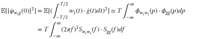
measured over a symmetric interval ![]() where the waveform g(t) can be conveniently considered a realization of a stochastic process characterized by the autocorrelation
where the waveform g(t) can be conveniently considered a realization of a stochastic process characterized by the autocorrelation ![]() (but the sample waveform is not known!) and its power spectral density
(but the sample waveform is not known!) and its power spectral density ![]() . Additive impairments w1(t) and w2(t) are Gaussian and uncorrelated with the waveform. The obvious choice is to resume the cross‐correlation estimator (20.1) by using one signal as reference for the other, this is evaluated first in terms of performance. Later in the section, the elegant and rigorous MLE for DToD will be derived.
. Additive impairments w1(t) and w2(t) are Gaussian and uncorrelated with the waveform. The obvious choice is to resume the cross‐correlation estimator (20.1) by using one signal as reference for the other, this is evaluated first in terms of performance. Later in the section, the elegant and rigorous MLE for DToD will be derived.
20.3.1 Correlation Method for DToD
In DToD, what matters is the relative ToD of one signal wrt the other as the two measurements are equivalent, and there is no preferred one. The cross‐correlation method is

where the two signals are shifted against one another until the similarities of the two signals are proved by the cross‐correlation metric. For discrete‐time sequences, the method can be adapted either to evaluate the correlation for the two discrete‐time signals, or to interpolate the signals while correlating (Appendix B). Usually the (computationally expensive) interpolation is carried out as second step after having localized the delay and a further ToD estimation refinement becomes necessary for better accuracy.
Performance Analysis
The cross‐correlation among two noisy signals (20.5) is expected to have a degradation wrt the conventional correlation method for ToD, at least for the superposition of noise and the unknown waveform. Noise is uncorrelated over the two sensors, ![]() for every α, but it has the same statistical properties. The MSE performance is obtained by considering the cross‐correlation for all the terms that concur in s1(t) and s2(t):
for every α, but it has the same statistical properties. The MSE performance is obtained by considering the cross‐correlation for all the terms that concur in s1(t) and s2(t):

and using a sensitivity analysis around the estimated value ![]() of DToD that peaks the cross‐correlation, from the derivative:
of DToD that peaks the cross‐correlation, from the derivative:
Recall that ![]() is the sample estimate of the stochastic cross‐correlation for a stationary process:
is the sample estimate of the stochastic cross‐correlation for a stationary process:

To simplify the notation, let the DToD be ![]() ; then the derivative of the correlation can be expanded into terms2
; then the derivative of the correlation can be expanded into terms2
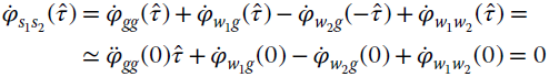
where the Taylor series has been applied only for the deterministic term on true DToD (![]() ):
): ![]() . For performance analysis of DToD, it is better to neglect any fluctuations of the second order derivative of the correlation of the waveform, which are replaced by its mean value
. For performance analysis of DToD, it is better to neglect any fluctuations of the second order derivative of the correlation of the waveform, which are replaced by its mean value ![]() , and thus
, and thus

It is now trivial to verify that the DToD is unbiased, while its variance (see properties in Appendix A, with ![]() )
)
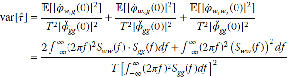
depends on the power spectral densities of stochastic waveform Sgg(f) and noise Sww(f). Once again, the effective bandwidth for stochastic processes for signal and noise

plays a key role in the DToD method. When considering bandlimited processes sampled at sampling interval Δt and bandwidth smaller than 1/2Δt (Nyquist condition), the effective bandwidth can be normalized to the sampling frequency to link the effective bandwidth for the sampled signal (say ![]() or
or ![]() for signal and noise)
for signal and noise)

Some practical examples can help to gain insight.
DToD for Bandlimited Waveforms
Let the noise be spectrally limited to Bw in Hz, with power spectral density ![]() for
for ![]() , and the spectral power density of the waveform upper limited to Bg (to simplify,
, and the spectral power density of the waveform upper limited to Bg (to simplify, ![]() ) with signal to noise ratio
) with signal to noise ratio

The variance of DToD from (20.6) is

This decreases with the observation length T and ρ, when the term in brackets is negligible as for large ρ, or when the noise is wideband (![]() ) and the ratio
) and the ratio ![]() cannot be neglected anymore. For small signal to noise ratio it decreases as 1/ρ2.
cannot be neglected anymore. For small signal to noise ratio it decreases as 1/ρ2.
Another relevant example is when all processes have the same bandwidth (![]() ) with the same power spectral density S(f) up to a scale factor:
) with the same power spectral density S(f) up to a scale factor: ![]() , when
, when
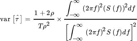
From the Schwartz inequality  , the variance is lower bounded by

This value is attained only for ![]() const.
const.
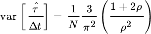
The case of time sequences with white Gaussian noise can be derived from the results above. In this case the overall number of samples is ![]() with noise bandwidth
with noise bandwidth ![]() and power
and power ![]() . The effective bandwidth of the noise is
. The effective bandwidth of the noise is ![]() and for the signal is
and for the signal is ![]() so that the variance of DToD follows from (20.7):
so that the variance of DToD follows from (20.7):

When considering sampled signals, it is more convenient to scale the variance to the sample interval so as to have the performance measured in sample units:

This depends on the number of samples (N) and the signal to noise ratio ρ; again the term 1/ρ2 disappears for large ρ. In the case that both waveform and noise are white (![]() ),
), ![]() and thus
and thus
More details on DToD in terms of bias (namely when ![]() ) and variance are in [96].
) and variance are in [96].
20.3.2 Generalized Correlation Method
The cross‐correlation method for DToD is the most intuitive extension of ToD, but there is room for improvement if rigorously deriving the DToD estimator from ML theory. Namely, the ML estimator was proposed by G.C. Carter [97] who gave order to the estimators and methods discussed within the literature of the seventies. We give the essentials here while still preserving the formal derivations.
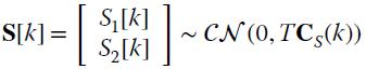
The basic assumption is that the samples of the Fourier transform of data si(t) (for ![]() ) evaluated at frequency binning
) evaluated at frequency binning ![]()
are zero‐mean Gaussian random variables. Provided that T is large enough to neglect any truncation effect due to the DToD τ (see Section 20.4), the correlation depends on the cross‐spectrum
and it follows that
is uncorrelated vs. frequency bins. The rv at the k th frequency bin is
where

The set of rvs for all the N frequency bins ![]() are Gaussian and independent, and the log‐likelihood is (apart from constant terms)
are Gaussian and independent, and the log‐likelihood is (apart from constant terms)

Still considering a large interval T, the ML metric for ![]() becomes
becomes

where the dependency on the DToD τ is in the phase of S(f) as
The inverse of the covariance

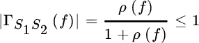
depends on the coherence of the two rvs defined as:
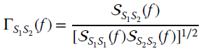
The ML metric ![]() (τ) can be expanded (recall the property:
(τ) can be expanded (recall the property: ![]() ) to isolate only the delay‐dependent term:
) to isolate only the delay‐dependent term:
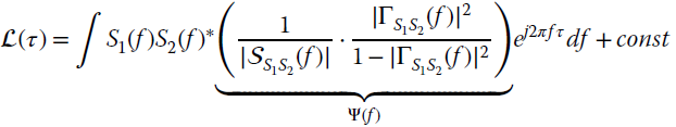
The MLE is based on is the search for the delayed cross‐correlation of the two signals (term ![]() ) after being filtered by Ψ(f). In practice, the DToD is by the correlation method provided that the two signals are preliminarily filtered by two filters H1(f) and H2(f) such that
) after being filtered by Ψ(f). In practice, the DToD is by the correlation method provided that the two signals are preliminarily filtered by two filters H1(f) and H2(f) such that ![]() as sketched in Figure 20.4.
as sketched in Figure 20.4.
Figure 20.4 Generalized correlation method.
Filter Design
Inspection of the coherence term based on the problem at hand
shows that it depends on the signal to noise ratio for every frequency bin
and it can be approximated as
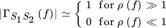
it downweights the terms when noise dominate the signal. The filter Ψ(f) is
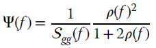
and a convenient way to decouple Ψ(f) into two filters is

where the first term decorrelates the signal for the waveform, and the second term accounts for the signal to noise ratio. If ρ(f) is independent of frequency, the second term is irrelevant for the MLE of DToD.
CRB for DToD
CRB can be derived from the log‐likelihood term that depends on the delay (20.10) and it follows from the definitions in Section 8.1:

or compactly
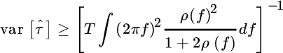
To exemplify, consider the case where signal and noise have the same bandwidth (e.g., this might be the case that lacks of any assumption on what is signal and what is noise, and measurements are prefiltered within the same bandwidth to avoid “artifacts”) ![]() with
with ![]() (i.e., this does not imply that
(i.e., this does not imply that ![]() const), then
const), then

coincides with the variance of correlation estimator (20.8) derived from a sensitivity analysis, except that any knowledge of the power spectral density of the waveform ![]() could use now the prefiltering (20.11) to attain an improved performance for the DToD correlator. If sampling the signals at sampling interval
could use now the prefiltering (20.11) to attain an improved performance for the DToD correlator. If sampling the signals at sampling interval ![]() (i.e., maximal sampling rate compatible with the processes here), the sequences have
(i.e., maximal sampling rate compatible with the processes here), the sequences have ![]() samples in total and the CRB coincides with (20.9).
samples in total and the CRB coincides with (20.9).
Even if the generalized correlation method is clearly the MLE for DToD, there are some aspects to consider when planning its use. The filtering (20.11) needs to have a good control of the model, and this is not always the case as the difference ToD is typically adopted in passive sensing systems where there is poor control of the waveform from the source, and the use of one measurement as reference for the others is a convenient and simple trick, namely when measurements are very large. In addition, the filtering introduces edge effects due to the filters’ transitions h(t) that limits the valid range T of the measurements. When filters are too selective, the filter response h(t) can be too long for the interval T and the simple correlation method (20.5) is preferred.
20.4 Numerical Performance Analysis of DToD
Performance of DToD depends on the observation interval T as this establishes the interval where the two waveforms maximally correlate. However, in the case that the true DToD τ is significantly different compared to T (Figure 20.5), the overlapping region within the area showing the same delayed waveform reduces by ![]() and thus the variance (20.8) scales accordingly as the non‐overlapped region acts as self‐noise:
and thus the variance (20.8) scales accordingly as the non‐overlapped region acts as self‐noise:

Figure 20.5 Truncation effects in DToD.
The same holds for any variance computation. This loss motivates the choice of “slant windowing” whenever one has the freedom to choose the two portions of observations s1(t) and s2(t) to correlate.
Measurements are usually gathered as sampled and all methods above need to be implemented by taking the sampling into account. Correlation for sampled signals needs to include the interpolation and resampling as part of the DToD estimation step as for the ToD method. However, the filtering might introduce artifacts that in turn degrade the overall performance except for the case when the DToD is close to zero. This is illustrated in the example below by generating a waveform from a random process with PSD within ![]() and white noise (
and white noise (![]() ). The signal is generated by filtering a white stochastic process with a Butterworth filter of order 8, and the second signal has been delayed using the DFT for fractional delay (see Appendix B). The fractional delay is estimated by using the parabolic regression discussed in Section 9.4. Below is the Matlab code for the Montecarlo test to evaluate the performance wrt the CRB.
). The signal is generated by filtering a white stochastic process with a Butterworth filter of order 8, and the second signal has been delayed using the DFT for fractional delay (see Appendix B). The fractional delay is estimated by using the parabolic regression discussed in Section 9.4. Below is the Matlab code for the Montecarlo test to evaluate the performance wrt the CRB.
Figure 20.6 shows the performance in terms of RMSE (measured in samples) compared to the CRB (dashed lines) for varying choices of the delay ![]() and
and ![]() samples. The performance attains the CRB for large SNR and
samples. The performance attains the CRB for large SNR and ![]() , while there is a small bias that justifies the floor for large SNR due to the parabolic regression on correlation evaluated for discrete‐time signals.
, while there is a small bias that justifies the floor for large SNR due to the parabolic regression on correlation evaluated for discrete‐time signals.

Figure 20.6 RMSE vs. SNR for DToD (solid lines) and CRB (dashed line).
20.5 Wavefront Estimation: Non‐Parametric Method (L=1)
When the waveform is not known and the measurements are highly redundant (![]() ), the wavefront can be estimated by iterated DToD among all measurements [98] even if, because of small waveform distortion vs. distance (see Figure 20.8), it would be preferable to use the DToD of neighboring signals. The set of delayed waveforms over a wavefront
), the wavefront can be estimated by iterated DToD among all measurements [98] even if, because of small waveform distortion vs. distance (see Figure 20.8), it would be preferable to use the DToD of neighboring signals. The set of delayed waveforms over a wavefront
depends on two geometrical parameters x, y according to the planar coordinates of the sensors (see Figure 20.7). For every pair of sensors out of M, say i and j at geometrical positions pi and pj, the correlation estimator on s(t; pi) and s(t; pj) yields the estimate of the DToD Δτi,j that is dependent on the DToD of the true delays
apart from an error αi,j that depends on the experimental settings (waveform, noise, any possible distortion, and even delays) as proved in (20.12).
Figure 20.7 Wavefront estimation from multiple DToD.
All the pairs that are mutually correlated can be used to estimate the DToDs up to a total of ![]() estimates (if using all‐to‐all pairs) to build a linear system
estimates (if using all‐to‐all pairs) to build a linear system
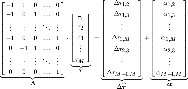
where the matrix ![]() has values
has values ![]() along every row to account for the pair of sensors used in DToD, and all the other terms have obvious meanings. Assuming that the DToD estimates are
along every row to account for the pair of sensors used in DToD, and all the other terms have obvious meanings. Assuming that the DToD estimates are
then the LS estimate of the ensemble of ToDs is
Notice that the wavefront ![]() is estimated up to an arbitrary translation as DToDs are not sensitive to a constant, and this reflects to a null eigenvalue of ATA that calls for the LS estimate using the pseudoinverse (Section 2.7). Any iterative estimation method for the solution of the LS estimate (e.g., iterative methods in Section 2.9) are not sensitive to null eigenvalues as that part of the solution in
is estimated up to an arbitrary translation as DToDs are not sensitive to a constant, and this reflects to a null eigenvalue of ATA that calls for the LS estimate using the pseudoinverse (Section 2.7). Any iterative estimation method for the solution of the LS estimate (e.g., iterative methods in Section 2.9) are not sensitive to null eigenvalues as that part of the solution in ![]() corresponding to the eigenvector of the constant value of τ is not updated.
corresponding to the eigenvector of the constant value of τ is not updated.
20.5.1 Wavefront Estimation in Remote Sensing and Geophysics
In remote sensing and geophysical signal processing, the estimation of the wavefront of delays (in seismic exploration these are called horizons since they define the ToD originated by the boundary between different media, as illustrated at the beginning of this Chapter) is very common and of significant importance. Even if these remote sensing systems are usually active with known waveform, the propagation over the dispersive medium and the superposition of many backscattered echoes severely distort the waveform, and make it almost useless for ToD estimation. However, in DToD estimation the waveform is similarly distorted for two neighboring sensors. This is exemplified in Figure 20.8 where the waveforms are not exactly the same shifted copy, but there is some distortion both in wavefront and in waveform (see the shaded area that visually compares the waveforms at the center and far ends of the array).
Figure 20.8 Curved and distorted wavefront (upper part), and measured data (lower part).
One common way to handle these issues is by preliminarily selecting those pair of sensors where the waveforms are not excessively distorted between one another, and this reduces the number of equations associated with the selected pairs of the overdetermined problem (20.13) to be smaller than ![]() (all‐to‐all configuration). This has a practical implication as the number of scans can be
(all‐to‐all configuration). This has a practical implication as the number of scans can be ![]() as in the seismic image at the beginning in Figure 20.1, and the use of M2/2 would be intolerably complex. Selecting the K neighbors (say
as in the seismic image at the beginning in Figure 20.1, and the use of M2/2 would be intolerably complex. Selecting the K neighbors (say ![]() ) can reduce the complexity to manageable levels KM/2. If M is not excessively large, one could still use all the
) can reduce the complexity to manageable levels KM/2. If M is not excessively large, one could still use all the ![]() pairs and account separately for the waveform distortion by increasing the DToD variance (20.12). As a rule of thumb, the distortion increases with the sensors’ distance
pairs and account separately for the waveform distortion by increasing the DToD variance (20.12). As a rule of thumb, the distortion increases with the sensors’ distance ![]() , and this degrades the variance proportionally
, and this degrades the variance proportionally

for an empirical choice of the scaling term η and exponent γ.
It is quite common to have outliers in DToD and this calls for some preliminary data classification (Chapter 23). In addition to the robust estimation methods (Section 7.9), another alternative is to solve for (20.13) by using an L1 norm. These methods are not covered here as they are based on the specific application, but usually they are not in closed form even if the optimization is convex, and are typically solved by iterative methods.
20.5.2 Narrowband Waveforms and 2D Phase Unwrapping
In narrowband signals, the waveform is the product of a slowly varying envelope a(t) with a complex sinusoid:
where ωo is the angular frequency. The delays are so small compared to the envelope variations that the signals at the sensors (i, j) are
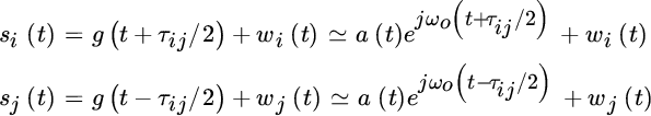
and the correlator‐based DToD estimator (neglecting the noise only for the sake of reasoning)
yields the estimate of the phase difference
that is directly related to the DToD. Wavefront estimation is the same as above with some adaptations [99]: phase difference (and phase in general3) is defined modulo‐ 2π from the arg[.] of the correlation of signals. Since ![]() phase is wrapped within
phase is wrapped within ![]() (herein indicated as [.]2π) so that the true measured phase difference differs from the true one by multiple of 2π, unless
(herein indicated as [.]2π) so that the true measured phase difference differs from the true one by multiple of 2π, unless ![]() . 2D phase unwrapping refers to the estimation of the continuous phase‐function
. 2D phase unwrapping refers to the estimation of the continuous phase‐function
(or the wavefront ![]() ) from the phase‐differences (20.14) evaluated modulo‐ 2π (also called wrapped phase). The LS unwrapping is similar to problem (20.13) by imposing for any pair of measurements the equality
) from the phase‐differences (20.14) evaluated modulo‐ 2π (also called wrapped phase). The LS unwrapping is similar to problem (20.13) by imposing for any pair of measurements the equality
in the LS sense. The system becomes
that yields the LS solution
Since phase is measured modulo‐ 2π, the choice of the sensor’s pairs is not extended to all the sensors, but rather to the neighborhood of each sensor as the phase‐variation among neighbor sensors is expected to be mostly smaller than π.
The concept of phase aliasing is illustrated by the example in Figure 20.9 where phase ϑi increases along the sensors’ position and the wrapped phase [ϑi]2π has 2π jumps when close to ![]() . If considering the angular difference of the phase between two points coarsely sampled 1:2 (gray points with double‐spacing
. If considering the angular difference of the phase between two points coarsely sampled 1:2 (gray points with double‐spacing ![]() ), the modulo‐ 2π value coincides with the true value except where phase difference
), the modulo‐ 2π value coincides with the true value except where phase difference ![]() (gray lines) while the wrapped phase difference
(gray lines) while the wrapped phase difference ![]() (i.e., the wrapped phase difference can be considered as the smallest angular difference between two consecutive vectors). Since the phase difference estimated from the wrapped phase differs from the true one by (a multiple of) 2π, there is no way to retrieve these
(i.e., the wrapped phase difference can be considered as the smallest angular difference between two consecutive vectors). Since the phase difference estimated from the wrapped phase differs from the true one by (a multiple of) 2π, there is no way to retrieve these ![]() jumps that impair the overall estimated phase‐function by the unwrapping algorithm. This is called phase aliasing condition. If sampling is dense enough (gray and black points in Figure 20.9), the phase‐differences are likely to be coincident with the true (unwrapped) phase without any artifacts.
jumps that impair the overall estimated phase‐function by the unwrapping algorithm. This is called phase aliasing condition. If sampling is dense enough (gray and black points in Figure 20.9), the phase‐differences are likely to be coincident with the true (unwrapped) phase without any artifacts.

Figure 20.9 Phase‐function and wrapped phase in  from modulo‐ 2π.
20.5.3 2D Phase Unwrapping in Regular Grid Spacing
In addition to wavefront estimation, 2D phase unwrapping has several notable applications in magnetic resonance imaging, optical interferometry, and satellite synthetic aperture radar (SAR) imaging. All these applications collect measurements over a regular grid spacing and the phase‐differences (20.15) are computed between neighboring points along two orthogonal directions. Since the transformation A is the derivative along the two dimensions, the phase differences can be partitioned along these two directions as
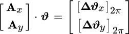
so that the LS estimate becomes
which can be solved efficiently by exploiting the structure of the linear operators and their sparsity—see Appendix C.
Inspection of the term ![]() shows that it contains the second order derivatives (i.e., discrete Laplace operator) of the unwrapped phase field
shows that it contains the second order derivatives (i.e., discrete Laplace operator) of the unwrapped phase field ![]() , while the terms on the right of (20.18) are the first‐order derivatives of the phase‐differences. This is the basis for several detailed lines of thought on the impact of phase‐difference artifacts such as the 2π discontinuities on the final solutions. The reader is referred to the copious literature on this fascinating topic that deals with the phase field as a continuous field that is sampled, and phase unwrapping artifacts are the results of coarse sampling of these phase fields.
, while the terms on the right of (20.18) are the first‐order derivatives of the phase‐differences. This is the basis for several detailed lines of thought on the impact of phase‐difference artifacts such as the 2π discontinuities on the final solutions. The reader is referred to the copious literature on this fascinating topic that deals with the phase field as a continuous field that is sampled, and phase unwrapping artifacts are the results of coarse sampling of these phase fields.
The example in Figure 20.10 shows the consequences of phase aliasing from the wrapped phase image [ϑ(x, y)]2π using (20.18) when the phase image is down‐sampled 1:n (i.e., take one sample out of n in both directions) to simulate phase aliasing when evaluating phase‐differences. The estimated phase ![]() is (visually) not affected by 1:2 decimation even if some residual is still visible on residual
is (visually) not affected by 1:2 decimation even if some residual is still visible on residual ![]() , while it is more severely affected when decimation is larger, as for 1:5, most of the artifacts are in those areas where there is a sudden change of the phase‐function (e.g., in the face, where luminance is abruptly changing from black to white). Residuals for 1:2 or 1:5 show a pattern that resembles the electric field with dipoles, there is a close analytical relationship, but the explanation is beyond the scope of the introductory discussion.
, while it is more severely affected when decimation is larger, as for 1:5, most of the artifacts are in those areas where there is a sudden change of the phase‐function (e.g., in the face, where luminance is abruptly changing from black to white). Residuals for 1:2 or 1:5 show a pattern that resembles the electric field with dipoles, there is a close analytical relationship, but the explanation is beyond the scope of the introductory discussion.

Figure 20.10 Example of 2D phase unwrapping.
One might argue that the solution to these artifacts could be to oversample the wavefields, but this is not always possible as the sensors’ density is given by the application. The interpolation of phase images cannot provide the solution as unfortunately phase information is related to the dynamics of the phase and not (easily) to the spectrum of the signals. Since phase aliasing introduces missing 2π jumps that are smeared by the LS method as diffused error (see 1:5 decimation around the face with abrupt black‐white discontinuities), these can be interpreted as outliers that are surely not‐Gaussian and the L2‐norm can be replaced with L1 metrics, possibly iterated. There are methods that solve for the LS phase estimate by cosine‐transforms, but this method is questionable for small images due to the poor control of artifacts at the boundary as consequence of the periodicity of the cosine‐transformation.
20.6 Parametric ToD Estimation and Wideband Beamforming
The ToDs ![]() depend on a set of shape parameters that fully characterize each waveform. A common and intuitive, but not unique, example is the wavefield originated by point sources at distances hℓ from a linear array of sensors located at
depend on a set of shape parameters that fully characterize each waveform. A common and intuitive, but not unique, example is the wavefield originated by point sources at distances hℓ from a linear array of sensors located at ![]() (see Figure 20.11). The 2D ray‐geometrical model of propagation in a homogeneous medium with propagating velocity v (in m/s) gives the hyperbolic ToD vs. array space x (here assumed as continuous just to ease the notation) in the two equivalent formulations:
(see Figure 20.11). The 2D ray‐geometrical model of propagation in a homogeneous medium with propagating velocity v (in m/s) gives the hyperbolic ToD vs. array space x (here assumed as continuous just to ease the notation) in the two equivalent formulations:
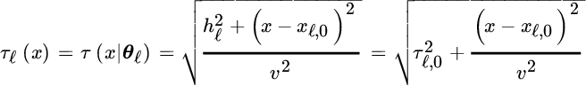
where the two shape parameters
are the geometrical position of the source, or alternatively when v is not known, the ToD at the vertex of the hyperbola ![]() :
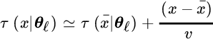
: ![]() . Note that in general, the wavefront is curved and, for large distances (far‐field approximation for the wavefront)
. Note that in general, the wavefront is curved and, for large distances (far‐field approximation for the wavefront) ![]() , it is linear with a slope
, it is linear with a slope
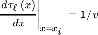
that depends on the slowness 1/v of the propagating medium. The example in Figure 20.11 shows the wavefields from 3 sources for wideband g(t) (left) and narrowband waveforms, and wideband s(x, t) with white noise or the same after filtering the noisy wavefield within the bandwidth of the signal. All slopes of the wavefronts are below the value defined by the propagation velocity ![]() 1500 m/s that mimics the acoustic waves in water as for a sonar sensing system, and hyperbolic ToDs
1500 m/s that mimics the acoustic waves in water as for a sonar sensing system, and hyperbolic ToDs ![]() are indicated by the dashed lines superimposed on the wavefield
are indicated by the dashed lines superimposed on the wavefield ![]() in various settings.
in various settings.

Figure 20.11 Example of delayed waveforms (dashed lines) from three sources impinging on a uniform linear array.
Furthermore, there are applications such as in subsurface remote sensing where backscattered wavefields are used for depth imaging and the propagation velocity v is unknown and this becomes an additional parameter to be estimated—or even worse (but unfortunately very common in many geophysical seismic exploration applications), the propagating medium is not homogeneous, the wavefield is not spherical, and the wavefront deviates from the hyperbolic shapes of the Figure 20.11. In these contexts, the number of parameters of a parametric ToD model become very complex and this is not covered herein. However, the approach is still based on estimation of the deviations from a nominal hyperbolic ToD shape based on some initial assumptions of the propagation velocity.
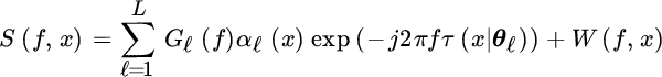
In complex contexts, there are many wavefronts impinging on an array of sensors and the signal at position ![]()
is characterized by the superposition of these delayed waveforms. The waveforms are not known but redundantly measured by the array to guarantee the possibility of estimating one waveform and mitigating (or attenuating) the others. Wideband beamforming refers to the method to delay and combine the multiple signals (20.19) to estimate the waveform of interest (say ![]() for the
for the ![]() ‐th wavefront), and possibly mitigate the others considered as interference.
‐th wavefront), and possibly mitigate the others considered as interference.
20.6.1 Delay and Sum Beamforming
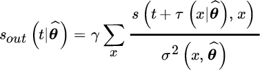
Delay and sum beamforming extends the beamforming methods in Chapter 19 to wideband waveforms. Making reference to the model (20.19), the wideband beamforming method delays each signal by a certain shape parameters ![]() and sums all the N delayed signals from all sensors:
and sums all the N delayed signals from all sensors:
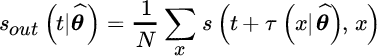
When the shape parameters match the ![]() th wavefield
th wavefield ![]() , this value flattens s(t, x) in (20.20) and the sum enhances it; the resulting signal becomes
, this value flattens s(t, x) in (20.20) and the sum enhances it; the resulting signal becomes

where the three terms are the signal of interest, interference from the other wavefronts (![]() ) that are reduced by the summing, and the noise that is reduced by 1/N. When
) that are reduced by the summing, and the noise that is reduced by 1/N. When ![]() , the signal is somewhat attenuated by the sum.
, the signal is somewhat attenuated by the sum.
Wideband beamforming is shown in the example in Figure 20.12 for a point source at ![]() and
and ![]() (or
(or ![]() as from the vertex of the hyperbolic wavefield) from the linear array, and propagation velocity is
as from the vertex of the hyperbolic wavefield) from the linear array, and propagation velocity is ![]() as for ultrasound systems with Ricker waveform (Section 9.4). The delay and sum beamforming
as for ultrasound systems with Ricker waveform (Section 9.4). The delay and sum beamforming ![]() is for varying source point
is for varying source point ![]() and the clearest waveform is when
and the clearest waveform is when ![]() as expected, with small artifacts when
as expected, with small artifacts when ![]() that decrease with N. The interference mitigation capability of delay and sum beamforming is shown for the same example when considering the presence on another interfering wavefield at
that decrease with N. The interference mitigation capability of delay and sum beamforming is shown for the same example when considering the presence on another interfering wavefield at ![]() and
and ![]() , and noise
, and noise ![]() is affected by the impairment, but surely much less than the original observation s(t, x).
is affected by the impairment, but surely much less than the original observation s(t, x).

Figure 20.12 Delay and sum beamforming for wideband signals.
The corresponding Matlab code for delay and sum beamforming described here follows, together with the generation of the signal (a gray‐scale image is used in place of wiggle plot in the figure, which enhances any waveform distortion after the sum).
Remark 1: The signal ![]() after the delay and sum beamforming is maximized for those choices of the shape parameters
after the delay and sum beamforming is maximized for those choices of the shape parameters ![]() that flattens the wavefields
that flattens the wavefields ![]() before summing up. The energy of
before summing up. The energy of ![]() within a predefined window can be used to estimate the presence or not of one source for a certain combination of shape parameters. The search is over the bidimensional pairs
within a predefined window can be used to estimate the presence or not of one source for a certain combination of shape parameters. The search is over the bidimensional pairs ![]() for the value(s) that peak(s) the energy metric, and time resolution is limited by the time window adopted in the energy metric.
for the value(s) that peak(s) the energy metric, and time resolution is limited by the time window adopted in the energy metric.
Remark 2: After delaying, the sum in (20.21) can take into account the different degree of noise and interference occurring in the flattened wavefield. This is obtained by weighting the terms before summing, and the weighting can be designed according to the degree of noise and interference that is experienced in the sum. The optimal weighting is the same as for BLUE (Section 6.5) and depends on the inverse of the power of the noise and interference ![]() for the specific shape parameters
for the specific shape parameters ![]() :
:
with normalization ![]()
20.6.2 Wideband Beamforming After Fourier Taransform
Implementation of delay and sum beamforming for discrete‐time signals needs to interpolate the signals when the delay is fractional. This is carried out by appropriate filtering as part of the delay for discrete‐time signals as detailed in Appendix B.
Alternatively, one can use the delay after the Fourier transform of the wavefields vs. time, which has several benefits. The model (20.19) after FT is
and, for every frequency, it is the superposition of spatial sinusoids each with appropriate spatial varying amplitudes αℓ(x). A wideband beamforming becomes:

and avoids any explicit interpolation step.
Another simplification of wideband modeling is for far‐field when the wavefront is planar, or around a certain position ![]() .
.
When the amplitude variations across space is negligible (![]() ) the model is
) the model is

where

These are the sum of spatial sinusoids that can be handled using the theory of narrowband array processing as illustrated in Chapter 19.
Appendix A: Properties of the Sample Correlations
Preliminarily, we can notice that for any WSS process x(t) the mean values can be evaluated as

where the last equality is due to the limited range of the autocorrelation within ![]() . If the interval T is much larger than the decorrelation of the process:
. If the interval T is much larger than the decorrelation of the process:

These approximations ease the computations of the terms:

that reduce to those in the main text.
Appendix B: How to Delay a Discrete‐Time Signal?
Fractional delay (not sample‐spaced) of a discrete‐time signal is very frequent in statistical signal processing. Let x1, x2, …, xN be a sequence to be delayed by τ samples, with τ non‐integer (otherwise, this would be simply a time‐shift of the samples) and sample index indicated by subscript. The solution is to interpolate the sequence with an appropriate continuous‐time interpolating function h(t) that estimates at best the continuous‐time signal:
assuming that the sampling interval is unitary. The interpolated signal ![]() can now be arbitrarily delayed
can now be arbitrarily delayed
and the delayed signal is uniformly resampled to have the delayed sequence:
The last equality shows that the delayed sequence is the convolution of the original sequence and the interpolating function delayed by τ and resampled.
Accuracy of fractional delay depends on the choice of the interpolating function h(t) that must honor the original samples (i.e., ![]() ) as discussed in Section 5.5. The ideal interpolating function
) as discussed in Section 5.5. The ideal interpolating function
is not commonly used as the tails decay too slowly and the sequence needs to be very long to avoid edge effects. One of the most common ways to interpolate is by using the spline (see the book by de Boor [100] for an excellent overview).
A very pragmatic way to delay a sequence is by the use of the discrete Fourier transform (DFT) under the assumption of periodicity of the sequence. Namely, from the sequence x1, x2, …, xN, the DFT is computed and the result in turn is delayed by a linear phase:

In spite of its simplicity, there are pitfalls to be considered to avoid “surprises” after fractional delays. Namely, the use of the DFT still uses an interpolation, which can be easily seen from the definition of the inverse DFT of Y(k):

which is periodic over N samples. Namely, when using the DFT all sequences are periodic, even if not originally. If the delay τ is small and the original sequence tapered to zero, these wrap‐around effects are negligible. Alternatively, the original sequence can be padded by zeros up to N′ (with ![]() ) to make the implicit periodic sequence long enough to reduce these artifacts (but still not zero after non‐fractional delays). Needless to say, the DFT must be computed with basis N′.
) to make the implicit periodic sequence long enough to reduce these artifacts (but still not zero after non‐fractional delays). Needless to say, the DFT must be computed with basis N′.
Appendix C: Wavefront Estimation for 2D Arrays
Let ![]() denote the matrix of (unknown) delay function (bold font indicates matrix),
denote the matrix of (unknown) delay function (bold font indicates matrix), ![]() and
and ![]() the matrixes of gradients, and
the matrixes of gradients, and ![]() the shift matrix (i.e.,
the shift matrix (i.e., ![]() ). The ToD of the wavefront can be related to the DToD along the two directions for the neighboring points (gradients of the wavefront):
). The ToD of the wavefront can be related to the DToD along the two directions for the neighboring points (gradients of the wavefront):

or equivalently

where ![]() and
and ![]() are operators for the evaluation of the gradients from the wavefront
are operators for the evaluation of the gradients from the wavefront ![]() . The equation (20.23) represents an overdetermined set of
. The equation (20.23) represents an overdetermined set of ![]() linear equations and MN unknowns that can be rearranged using the properties of the Kronecker products (Section 1.1.1)
linear equations and MN unknowns that can be rearranged using the properties of the Kronecker products (Section 1.1.1)
here ![]() and
and ![]() . The LS wavefront estimator is
. The LS wavefront estimator is
or equivalently
which is the discrete version of the partial differential equation with boundary conditions [99], where ![]() (or
(or ![]() ) is the discrete version of the second order derivative along x (or y). The matrixes are large but sparse, and this can be taken into account when employing iterative methods for the solution (Section 2.9) that converge even if A is ill conditioned (i.e., the update rule is independent of any constant additive value).
) is the discrete version of the second order derivative along x (or y). The matrixes are large but sparse, and this can be taken into account when employing iterative methods for the solution (Section 2.9) that converge even if A is ill conditioned (i.e., the update rule is independent of any constant additive value).
The Matlab code below exemplifies how to build the numerical method to solve for the wavefront from the set of DToD, or for 2D phase unwrapping when the phase‐differences ![]() are evaluated modulo‐ 2π. Since all matrixes Dx and Dy are sparse, its is (highly) recommended to build these operators using the
are evaluated modulo‐ 2π. Since all matrixes Dx and Dy are sparse, its is (highly) recommended to build these operators using the sparse toolbox (or any similar toolbox).