
16
Line Spectrum Analysis
The estimation of the frequencies of multiple sinusoidal signals is remarkably important and common in engineering, namely for the Fourier analysis of observations or experiments that model the observations as random set of values whose statistical properties depend on the angular frequencies. Since the problem itself reduces to the estimation of the (angular) frequencies as a generalization of Section 9.2 and Section 9.3, one might debate the rationale of dedicating a whole chapter to this. The problem itself needs care in handling the assumptions behind every experiment and these were deliberately omitted in the early chapters. Crucial problems addressed here are (1) resolution (estimating two sinusoids with similar frequencies), (2) finding alternative methods to solve non‐linear optimizations, and (3) evaluating accuracy wrt the CRB. All these matters triggered several frantic research efforts around the ’80s in this scientific area. A strong boost was given by array processing (Chapter 19) as the estimation of the spatial properties of wavefields from multiple radiating sources in space is equivalent to the estimation of (spatial) angular frequencies, and resolution therein pertains to the possibility to spatially distinguish the emitters. Since MLE is not trivial, and closed form optimizations are very cumbersome, the scientific community investigated a set of so called high‐resolution (or super‐resolution1) methods based on some ingenious algebraic reasoning. All these high‐resolution estimators treated here are consistent and have comparable performance wrt the CRB, so using one or another is mostly a matter of taste, but the discussion of the methodological aspects is very useful to gain insight into these challenging methods. As elsewhere, this topic is very broad and it deserves more space than herein, so readers are referred to [62,65,66,101] (just to mention a few) for extensions to some of the cases not covered here, and for further details.
Why Line Spectrum Analysis?
The sinusoidal model is

where {Aℓ, ωℓ, ϕℓ} are amplitudes, angular frequencies, and phases. The problem at hand is the estimation of the frequencies {ωℓ} that are ![]() from a noisy set of observations {x[n]}. In radar, telecommunications, or acoustic signal processing, the complex‐valued form
from a noisy set of observations {x[n]}. In radar, telecommunications, or acoustic signal processing, the complex‐valued form

is far more convenient even if this form is not encountered in real life as it rather stands for manipulation of real‐valued measurements (Section 4.3). This is the model considered here and some of the assumptions need to be detailed.
The phases {ϕℓ} account for the initial value that depends on the origin (sample ![]() ) and they are intrinsically ambiguous (i.e., the set {Aℓ, ωℓ, ϕℓ} is fully equivalent to
) and they are intrinsically ambiguous (i.e., the set {Aℓ, ωℓ, ϕℓ} is fully equivalent to ![]() ). Phases are nuisance parameters that are conveniently assumed as random and independent so that
). Phases are nuisance parameters that are conveniently assumed as random and independent so that
and thus
It follows that the autocorrelation is
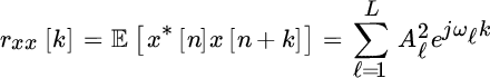
and the PSD is a line spectrum

as the sum of Dirac‐deltas. The signal affected by the additive white noise ![]()
![]() and the corresponding PSD is
and the corresponding PSD is
as illustrated in Figure 16.1. Spectrum analysis for line spectra refers to the estimation of the frequencies of x[n] assuming the model above.

Figure 16.1 Line spectrum analysis.
16.1 Model Definition
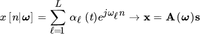
The data can be sliced into a set of N samples each (Figure 16.2), where t indexes the specific sample with ![]() that is usually referred to as time (e.g., this is the time in data segmentation as in Section 14.1.6, or time of independent snapshots of the same process as later in Chapter 19). The general model of the observations at time t is
that is usually referred to as time (e.g., this is the time in data segmentation as in Section 14.1.6, or time of independent snapshots of the same process as later in Chapter 19). The general model of the observations at time t is
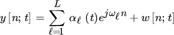
where ![]() collects amplitudes and phases that are arbitrarily varying (not known), and w[n; t] accounts for the noise. Since the variation of αℓ(t) vs. time t is usually informative of the specific phenomena, or encoded information, here this will be called signal (or source signal or simply amplitudes) as it refers to the informative signal at frequency ωℓ.
collects amplitudes and phases that are arbitrarily varying (not known), and w[n; t] accounts for the noise. Since the variation of αℓ(t) vs. time t is usually informative of the specific phenomena, or encoded information, here this will be called signal (or source signal or simply amplitudes) as it refers to the informative signal at frequency ωℓ.

Figure 16.2 Segmentation of data into N samples.
Each set of N observations, with ![]() , are collected into a vector that represents the compact model used for line spectra analysis
, are collected into a vector that represents the compact model used for line spectra analysis

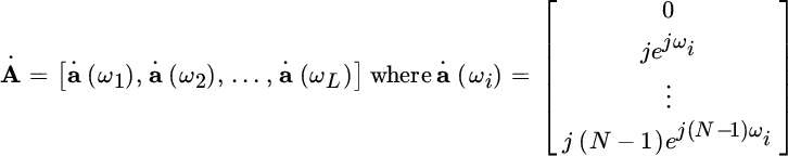
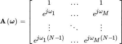
where
for the set of L angular frequencies
with signals
Noise is uncorrelated
and uncorrelated across time ![]() . This assumption does not limit the model in any way, as for correlated noise a pre‐whitening can reduce the model to the one discussed here (Section 7.5.2).
. This assumption does not limit the model in any way, as for correlated noise a pre‐whitening can reduce the model to the one discussed here (Section 7.5.2).
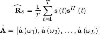
16.1.1 Deterministic Signals s (t)
Signals s(t) are nuisance parameters in line spectrum analysis and typically change vs. time index t but, once estimated the frequencies ω, the data {y(t)} can be written as a linear regression wrt {s(t)} and these are estimated accordingly. However, the way to model the nuisance s(t) contributes in defining the estimators and these are essentially modeled either as deterministic and unknown, or random. If deterministic, the set {s(t)} enters into the budget of the parameters to estimate as described in Section 7.2, and the model is
and the corresponding ML will be reviewed in Section 16.2. When {s(t)} are handled as random, the model deserves further assumptions detailed below.
16.1.2 Random Signals s (t)
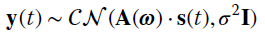
A reasonable (and common) assumption is that signals are random
where the zero‐mean is a direct consequence of the uniform phases {ϕℓ}, and the covariance Rs reflects the power of the signal associated with each sinusoid, and their mutual correlation. According to the random assumption of s(t), the data is modeled as
where the covariance
is structured according to the structure of A(ω) that in turn it depends on the (unknown) ω1, ω2, …, ωL, and mutual correlation among signals from Rs.
16.1.3 Properties of Structured Covariance
Let the columns of A(ω) be independent, or equivalently the frequencies be distinct (![]() for
for ![]() ); thus:
); thus:
or stated differently, the algebraic properties of A(ω)RsAH(ω) depend on the correlation properties of the sources with Rs. When all the signals are uncorrelated with arbitrary powers
the covariance of s(t) is full‐rank ![]() with
with
The eigenvalue decomposition is
but for the property (16.1), the eigenvalues in ![]() ordered for decreasing values are
ordered for decreasing values are
Rearranging the eigenvectors into the first L leading eigenvalues and the remaining ones
the basis
spans the same subspace of the columns of A(ω):
and this is referred to as signal subspace. To stress this point, there exists an orthonormal transformation (complex set of rotations) Q such that it transforms the columns of A(ω) into US:
with the known properties of the othornormal transformation ![]() .
.
The complementary basis
spans the noise subspace as complementary to signal subspace. This is clear when considering that the eigenvector decomposition of Ry is
and thus
The effect of the noise is only to increase the values of the eigenvalues, but not to change the subspace partitioning.
To exemplify, we can consider the following case for ![]() with
with ![]() :
:

For ![]() , the two signals are uncorrelated with
, the two signals are uncorrelated with ![]() , but increasing ρ makes the two signals correlated and
, but increasing ρ makes the two signals correlated and ![]() up to the case
up to the case ![]() for
for ![]() . But
. But ![]() is the case where the two signals are temporally fully correlated (the same source
is the case where the two signals are temporally fully correlated (the same source ![]() ) and the model becomes
) and the model becomes
where ![]() . In this case the column space of the two sinusoids cannot distinguish two signals even if the frequencies are distinct.
. In this case the column space of the two sinusoids cannot distinguish two signals even if the frequencies are distinct.
16.2 Maximum Likelihood and Cramér–Rao Bounds
MLE depends on the model and we can distinguish two methods for the two models:
- Conditional (or deterministic) ML (CML): in this case the nuisance parameters are deterministic and the model is
The parameters are
or more specifically the 3 L + 1 parameters:

with possibly time‐varying amplitudes and phases.
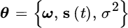
- Unconditional (or stochastic) ML (UML): the amplitudes s are nuisance parameters modeled as random (Section 7.4) and the model is
The parameters are

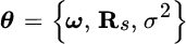
Overall the L + 1 parameters given by {ω, σ2} are augmented by the
 complex‐valued parameters of Rs (or L2 real‐valued) that are fewer than the L2 complex‐valued parameters due to symmetry.
Table 16.1 summarizes taxonomically the main results of this section (from [62,63,101] ) in terms of model, ML metrics, and CRB for the estimation of ω.
Table 16.1 Deterministic vs. stochastic ML in line spectrum analysis.
| Deterministic ML (CML) | Stochastic ML (UML) | |
| Model | ||
| ML | ||
| CRB(ω) | 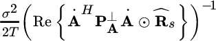 |
 |
 |
||
16.2.1 Conditional ML
This model has been widely investigated in Section 7.2 for multiple measurements and the CML follows from the optimization of
where ![]() is the projection onto ℛ{A(ω)} and
is the projection onto ℛ{A(ω)} and

is the sample correlation. For ![]() , the CML reduces to the frequency estimation in Section 9.2, but in general the optimization is not trivial, and various methods have been investigated in the past and are reproposed herein.
, the CML reduces to the frequency estimation in Section 9.2, but in general the optimization is not trivial, and various methods have been investigated in the past and are reproposed herein.
16.2.2 Cramér–Rao Bound for Conditional Model
Conditional Model for 
For ![]() (one observation), the CRB follows from the FIM for the Gaussian model
(one observation), the CRB follows from the FIM for the Gaussian model ![]() in Section 8.4.3:
in Section 8.4.3:

where
and noise power σ2 is assumed known. Parameters can be separated into amplitudes and phase so that the derivatives are

and for the L sinusoids the FIM is block‐partitioned; the size of each block is ![]()

and the entries are


The CRB in this way does not yield a simple closed form solution for the correlation between frequencies. Just to exemplify, the inner products are

where φmk is a phase‐term (not evaluated here). The degree of coupling among the different frequencies decreases provided that the frequency difference is ![]() , and for increasing N as
, and for increasing N as ![]() . Asymptotically with
. Asymptotically with ![]() , the frequencies are decoupled and the covariance is well approximated by the covariance for one sinusoid in Gaussian noise:
, the frequencies are decoupled and the covariance is well approximated by the covariance for one sinusoid in Gaussian noise: ![]() (See Section 9.2).
(See Section 9.2).
Conditional Model for 
For any T, a closed form for the frequency only was derived in [62] . More specifically, the CRB for the frequency is

where
is the sample correlation of the sources, and the derivatives are ![]() .
.
From the CRB one can obtain some asymptotic properties for ![]() and/or
and/or ![]() that are useful to gain insight into the pros and cons of the frequency estimation methods. Once the CRB has been defined as above (
that are useful to gain insight into the pros and cons of the frequency estimation methods. Once the CRB has been defined as above (![]() ), the following properties hold when
), the following properties hold when ![]() for
for ![]() (or T large enough) [62,63] :
(or T large enough) [62,63] :


where [Rs]ℓℓ/σ2 is the signal to noise ratio for the ℓ th source, and ![]() is the asymptotic CRB. The variance for the ℓ th frequency
is the asymptotic CRB. The variance for the ℓ th frequency ![]() using the CML is
using the CML is
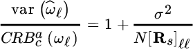
which proves that the CML is inefficient for ![]() even though
even though ![]() , and this makes the use of the conditional model questionable.
, and this makes the use of the conditional model questionable.
16.2.3 Unconditional ML
The model is
and the covariance is parametric:
The MLE is the minimizer of the cost function (Section 7.2)
for the sample correlation
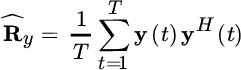
that has the property
from the law of large numbers or the stationarity of the measurements.
The minimization is very complex using the properties of derivative wrt matrix entries in Section 1.4. However, the minimization is separable in two steps [61] : first the log‐likelihood is optimized wrt Rs (i.e., for each entry of Rs) for a fixed ω to get a first estimate ![]() :
:
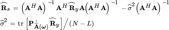
and then this is plugged into the log‐likelihood resulting in a function of ω only:
Minimization is not straightforward and one should use numerical methods.
16.2.4 Cramér–Rao Bound for Unconditional Model
The CRB has no compact and closed form and it can be derived by following the definitions (Section 7.2). A strong argument in favor of the CRB for the unconditional model is that the CRB is attained for ![]() as in standard ML theory. The CRB can be evaluated from the FIM (see Section 8.4.3)
as in standard ML theory. The CRB can be evaluated from the FIM (see Section 8.4.3)

To sketch the proof, which is very complex for the general case, let Rs be known (e.g., uncorrelated signals); the derivative

depends on the i th column of A(ω) as all the others are zero. The proof can be developed further for this special case, but we propose the general formula for FIM that was derived initially in [63] , and subsequently in [104] , for T observations:

Evaluation of the corresponding CRB needs to evaluate each of the terms of the FIM that can be simplified in some situations such as for uncorrelated sources (![]() ) and/or orthogonal sinusoids.
) and/or orthogonal sinusoids.
16.2.5 Conditional vs. Unconditional Model & Bounds
Conditional and unconditional are just two ways to account for the nuisance of complex amplitudes. Both methods are based on the sample correlation that averages all the T observations, provided that these are drawn from independent experiments with different signals s(t). Performance comparison between the two methods has been subject of investigations in the past and the main results are summarized below (from [63] ).
Let CRBu and CRBc be the CRB for unconditional and conditional models, and Cu and Cc the covariance matrix of the UML and CML; then the following inequalities hold:
This means that: [d)]
- CML is statistically less efficient than UML;
- UML achieves the unconditional CRB CRBu;
- CRBu is a lower bound on the asymptotic statistical accuracy of any (consistent) frequency estimate based on the data sample covariance matrix;
- CRBc cannot be attained.
In summary, the unconditional model has to be preferred as the estimate attains the CRBu while the estimate based on conditional model can only be worse or equal.
16.3 High‐Resolution Methods
Any of the MLE methods needs to search over the L‐dimensional space for frequencies, and this search could be cumbersome even if carried out as a coarse and fine search. High‐resolution methods are based on the exploration of the algebraic structure of the model in Section 16.1 and attain comparable performance to MLE, and close to the CRB. All these high‐resolution estimators are consistent with the number of observations T and have comparable performance.
16.3.1 Iterative Quadratic ML (IQML)
Iterative quadratic ML (IQML) was proposed by Y. Besler and A. Makovski in 1986 [64] to solve iteratively an optimization problem that is made quadratic after re‐parameterizing the cost function at every iteration. IQML is the conditional ML for T = 1, and generalization to any T is the algorithm MODE (Method for Direction Estimation) tailored for DoAs estimation (Chapter 19) [67].
Let ![]() be the linear transformation at the k th iteration; IQML solves at the k th iteration an objective where the non‐linear term in the kernel is replaced by the solution
be the linear transformation at the k th iteration; IQML solves at the k th iteration an objective where the non‐linear term in the kernel is replaced by the solution ![]() at iteration (k‐1):
at iteration (k‐1):
The optimization is wrt ωk, and then Ak to iterate until convergence. The advantage is that the optimization of Ψ(ωk) can become quadratic provided that the the cost function is properly manipulated by rewriting the optimization using a polynomial representation of the minimization.
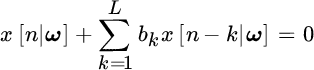
Given the signal
any filter represented in terms of z‐transform by the polynomial

is a linear predictor for ![]() and it is represented by a filter with
and it is represented by a filter with ![]() coefficients
coefficients ![]() with roots in
with roots in ![]() :
: ![]() for
for ![]() . Sinusoids are exactly predictable, so from the definition of prediction, any inner product between vector b and any subset of length
. Sinusoids are exactly predictable, so from the definition of prediction, any inner product between vector b and any subset of length ![]() extracted from
extracted from ![]() is zero. From the definition of the convolution matrix
is zero. From the definition of the convolution matrix

it follow that
From this identity, it follows that
and thus
The MLE becomes the estimation of the entries of b such that
from the noisy data ![]() .
.
Recalling the idea of IQML, this optimization becomes

where the convolution matrix ![]() is obtained at the previous iteration
is obtained at the previous iteration ![]() . The solution does not appear quadratic, but the product BHy is a convolution and it can be written alternatively as
. The solution does not appear quadratic, but the product BHy is a convolution and it can be written alternatively as
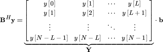
and so the optimization becomes quadratic
where
Notice that at every step of the minimization, there is the need to add a constraint to avoid the trivial solution ![]() . By adding the constraint that
. By adding the constraint that ![]() , the optimization reduces to a Rayleight quotient (Section 1.7) and the solution is the eigenvector associated with the minimum eigenvector of
, the optimization reduces to a Rayleight quotient (Section 1.7) and the solution is the eigenvector associated with the minimum eigenvector of ![]() ; this is denoted as IQML with quadratic constraint (IQML‐QC). Other constraints are
; this is denoted as IQML with quadratic constraint (IQML‐QC). Other constraints are ![]() (provided that it is not required to estimate a zero‐frequency component, or
(provided that it is not required to estimate a zero‐frequency component, or ![]() ). Alternatively
). Alternatively ![]() as there is a control of the position of the roots along the circle that is not controlled by IQML‐QC. In order to constrain roots along the unit circle of the z‐transform, it should at least have complex conjugate symmetry
as there is a control of the position of the roots along the circle that is not controlled by IQML‐QC. In order to constrain roots along the unit circle of the z‐transform, it should at least have complex conjugate symmetry ![]() (necessary, but not sufficient condition, see Appendix B of Chapter 4) and it follows from the overall constraints (there are L constraints if L is even) that the total number of unknowns of the quadratic problem is L. Furthermore, usually one prefers to rewrite the unknowns into a vector that collects real and imaginary components of bk:
(necessary, but not sufficient condition, see Appendix B of Chapter 4) and it follows from the overall constraints (there are L constraints if L is even) that the total number of unknowns of the quadratic problem is L. Furthermore, usually one prefers to rewrite the unknowns into a vector that collects real and imaginary components of bk: ![]() (assuming to constrain one sample of the complex conjugate symmetry
(assuming to constrain one sample of the complex conjugate symmetry ![]() and removing all the constraints from the optimization problem). This optimization is unconstrained and quadratic and it can be solved using QR factorization [67].
and removing all the constraints from the optimization problem). This optimization is unconstrained and quadratic and it can be solved using QR factorization [67].
IQML is not guaranteed to converge to the CML solution, and as for any iterative method, convergence depends on the initialization. The initialization ![]() implies that all frequencies are mutually orthogonal (e.g., the sinusoids have frequencies on the grid spacing 2π/N) but any other initialization that exploits the a‐priori knowledge of the frequencies (even if approximate) could ease the convergence.
implies that all frequencies are mutually orthogonal (e.g., the sinusoids have frequencies on the grid spacing 2π/N) but any other initialization that exploits the a‐priori knowledge of the frequencies (even if approximate) could ease the convergence.
16.3.2 Prony Method
This method was proposed by Prony more than two centuries ago (in 1795) and it is based on the predictability of sinusoids. Similar to the IQML method, for sinusoids:
Now the set of equations for the observations ![]() becomes
becomes

to estimate the frequencies from the roots: ![]() . The linear system requires that the number of observations are
. The linear system requires that the number of observations are ![]() , and for
, and for ![]() it is overdetermined (Section 2.7) and is appropriate when noise is high. Note that for L real‐valued sinusoids, the polynomial order is 2L and the full predictability needs
it is overdetermined (Section 2.7) and is appropriate when noise is high. Note that for L real‐valued sinusoids, the polynomial order is 2L and the full predictability needs ![]() observations.
observations.
16.3.3 MUSIC
MUSIC stands for multiple signal classification [65] and it is a subspace method based on the property that the first L eigenvectors associated with the leading eigenvalues of Ry is a basis of the columns of A(ω) detailed in Section 16.1.3. Considering the sample correlation

one can extend the subspace properties as ![]() for
for ![]() . Let the eigenvector decomposition
. Let the eigenvector decomposition ![]() , the L eigenvectors
, the L eigenvectors ![]() associated to the leading eigenvalues span the signal subspace:
associated to the leading eigenvalues span the signal subspace:
or alternatively, the remaining eigenvectors ![]() span the noise subspace
span the noise subspace
where “![]() ” highlights that the equality is exact only asymptotically as
” highlights that the equality is exact only asymptotically as ![]() for
for ![]() . According to geometrical similarity,
. According to geometrical similarity, ![]() is the basis of the signal subspace and
is the basis of the signal subspace and ![]() is the complementary basis of noise subspace drawn from the limited T observations. From the decomposition, the orthogonality condition
is the complementary basis of noise subspace drawn from the limited T observations. From the decomposition, the orthogonality condition
follows, which is useful for frequency estimation.
MUSIC is based on the condition above rewritten for each sinusoid
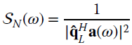
According to this property for the noise subspace basis, one can use a trial‐sinusoid a(ω) to have the noise spectrum
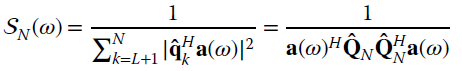
and the frequencies are obtained by picking the L values of ω that maximize the noise spectrum ![]() , as for those values the denominator approaches zero. Note that the noise spectrum is characterized by a large dynamic and coarse/fine search strategies are recommended—but still of one variable only.
, as for those values the denominator approaches zero. Note that the noise spectrum is characterized by a large dynamic and coarse/fine search strategies are recommended—but still of one variable only.
Root‐MUSIC
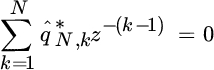
There are several variants of the MUSIC algorithm. One can look at the noise spectrum as a search for a frequency that nulls ![]() , but this can be replaced by searching for the L pairs of roots {zℓ} in reciprocal position wrt the unit circle over the 2N roots of the polynomial
, but this can be replaced by searching for the L pairs of roots {zℓ} in reciprocal position wrt the unit circle over the 2N roots of the polynomial

where
Since
the frequency follows from the angle of these roots:

Pisarenko Method
This method was proposed in 1973 by Pisarenko when solving geophysical problems [66] and it is the first example of a subspace method, which inspired all the others. It is basically MUSIC with ![]() , and thus the noise subspace is spanned by one vector only. Since
, and thus the noise subspace is spanned by one vector only. Since ![]() , the noise spectrum is
, the noise spectrum is
The root‐method reduces to the search for the L roots of the polynomial
with frequencies being the corresponding phases.
MUSIC vs. CRB
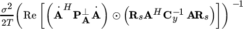
MUSIC is a consistent estimator and performance was investigated by the seminal work of Stoica and Nehorai [62] . Once again, the closed form of the covariance reveals some properties of the estimator, but more importantly the comparison with CRB highlights the consistency. Basically, the performance for ![]() is more simple and meaningful as this reflects the asymptotic performance. The CRB and the covariance of MUSIC are
is more simple and meaningful as this reflects the asymptotic performance. The CRB and the covariance of MUSIC are
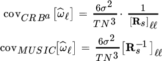
so the ratio
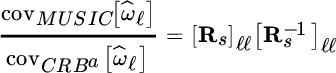
increases when Rs is singular, or sources are correlated. On the other hand, for uncorrelated sources ![]() , and this motivates its widespread use in this situation. To conclude, great care should be taken when using MUSIC as to the degree of correlation of sources.
, and this motivates its widespread use in this situation. To conclude, great care should be taken when using MUSIC as to the degree of correlation of sources.
Resolution
One of the key aspect of subspace methods such as MUSIC is the large resolution capability. An example can illustrate this aspect. Let ![]() be the frequencies of three sinusoids with unit amplitudes and statistically independent phases (MUSIC attains the CRBa in this case); the noise has power
be the frequencies of three sinusoids with unit amplitudes and statistically independent phases (MUSIC attains the CRBa in this case); the noise has power ![]() . The frequencies of the two sinusoids are so closely spaced so that they can only be resolved by the periodogram if (necessary condition)
. The frequencies of the two sinusoids are so closely spaced so that they can only be resolved by the periodogram if (necessary condition)
Figure 16.3 shows the comparison between the periodogram when using a segmentation of ![]() samples (solid line) and MUSIC using
samples (solid line) and MUSIC using ![]() samples (dashed line); details around the dashed box are magnified. The periodogram cannot distinguish two local maxima as they are too close even for
samples (dashed line); details around the dashed box are magnified. The periodogram cannot distinguish two local maxima as they are too close even for ![]() , while MUSIC has two well‐separated maxima at the two frequencies even for just
, while MUSIC has two well‐separated maxima at the two frequencies even for just ![]() samples. On increasing N, the maxima are even more separated (for the sake of plot clarity the total number of samples here are
samples. On increasing N, the maxima are even more separated (for the sake of plot clarity the total number of samples here are ![]() , simply to average the estimates from 20 Montecarlo trials).
, simply to average the estimates from 20 Montecarlo trials).

Figure 16.3 Resolution of MUSIC (dashed line) vs. periodogram (solid line).
16.3.4 ESPRIT
Estimation of signal parameters via rotational invariance techniques (ESPRIT) was proposed by Roy and Kailath [68] and it is based on the generalization of the predictability of sinusoids. To introduce the idea, let N observations x be noise‐free as superposition of L sinusoids with ![]() . If partitioning these observations into two subsets of the first and the last
. If partitioning these observations into two subsets of the first and the last ![]() observations:
observations:
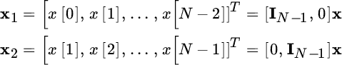
the subset x2 can be derived from x1 by applying to the subset x1 a phase‐shift to each sinusoid that depends on its frequency, and thus to all sinusoids. If rewriting all to set this phase‐shift as an unknown parameter, estimating the phase‐shifts to match x1 and x2 is equivalent in estimating the frequency of all sinusoids. Moving to a quantitative analysis:

where B1 and B2 are obtained by stripping the first and the last row of
To exemplify, when removing one sample (say the last) for one sinusoid with frequency ![]() , the same data can be resumed by multiplying all the samples by a frequency‐dependent term:
, the same data can be resumed by multiplying all the samples by a frequency‐dependent term:
that makes the shifted vector coincident with the signal when removing the first sample. It is straightforward to generalize this property
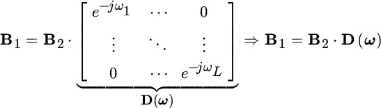
where
maps from x2 onto x1 by a proper set of phase‐shifts D(ω) that depend on the unknown frequencies.
In practice, one cannot act on A(ω) as it is unknown, but rather it is possible to act on the basis US of signal subspace that is obtained from the covariance matrix ![]() (in practice from
(in practice from ![]() ). The two matrixes are dependent on one other according to an orthonormal transformation C:
). The two matrixes are dependent on one other according to an orthonormal transformation C: ![]() . Stripping the first and last row from the basis of the signal subspace US gives:
. Stripping the first and last row from the basis of the signal subspace US gives:
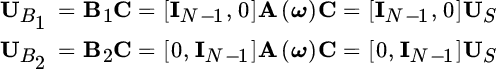
since
Multiplying both sides of ![]() for C yields
for C yields
and thus
Revisiting this relationship, it follows that ESPRIT estimation of the frequencies as the phases of the eigenvalues follows from the eigenvalue/eigenvector decomposition of the (unknown) ![]() that maps (by a rotation of the components)
that maps (by a rotation of the components) ![]() onto
onto ![]() .
.
All that remains is the estimation of the transformation ![]() , which can be obtained by the LS solution
, which can be obtained by the LS solution
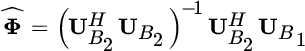
and thus from the eigenvalues of ![]() one gets the frequencies as those phases of the L eigenvalues closer to the unit circle. Notice that the LS estimate of
one gets the frequencies as those phases of the L eigenvalues closer to the unit circle. Notice that the LS estimate of ![]() searches for the combination of
searches for the combination of ![]() that justifies (in the LS‐sense)
that justifies (in the LS‐sense) ![]() , and any mismatch is attributed to
, and any mismatch is attributed to ![]() . However, for the problem at hand, both
. However, for the problem at hand, both ![]() and
and ![]() are noisy as they were obtained from noisy observations, and thus any mismatch is not only due to one of the terms. The LS can be redefined in this case and the total LS (TLS) should be adopted as mandatory for ESPRIT [68].
are noisy as they were obtained from noisy observations, and thus any mismatch is not only due to one of the terms. The LS can be redefined in this case and the total LS (TLS) should be adopted as mandatory for ESPRIT [68].
Remark
ESPRIT is more general than only referring to the first and last row of the data vector. It is sufficient that the following property holds:
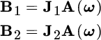
for any pair of selection matrixes J1 and J2 (with ![]() ) of the same dimension
) of the same dimension ![]() with
with ![]() such that the two subsets differ only by a rigid translation that maps onto a frequency‐dependent phase‐shift.
such that the two subsets differ only by a rigid translation that maps onto a frequency‐dependent phase‐shift.
16.3.5 Model Order
Many details have been omitted up to now as being simplified or neglected, but when dealing with real engineering problems one cannot avoid the details as the results might have surprises. The methods above are the most used; others have been proposed in the literature with some differences. However, all the estimators assume that the number of frequencies L is known, and this is not always true in practical problems. The number of sinusoids is called the model order and its knowledge is as crucial as the estimator itself. Under‐estimating the model order misses some sinusoids, mostly those closely spaced apart, while over‐estimating might create artifacts. Using the same example in Figure 16.3 with three sinusoids in noise of MUSIC, the noise spectrum when over‐estimating the order (say estimating ![]() frequencies when there are
frequencies when there are ![]() sinusoids) shows the spectrum with some peaks that add to the peaks of the true sinusoids. This is illustrated in Figure 16.4 for a set of 30 Montecarlo trials with the same situations as the MUSIC example (Figure 16.3).
sinusoids) shows the spectrum with some peaks that add to the peaks of the true sinusoids. This is illustrated in Figure 16.4 for a set of 30 Montecarlo trials with the same situations as the MUSIC example (Figure 16.3).
Figure 16.4 MUSIC for four lines from three sinusoids (setting of Figure 17.3).
There are criteria for model order selection based on the analysis of the eigenvalues of the sample correlation matrix ![]() . Namely, the eigenvalues ordered for decreasing values are
. Namely, the eigenvalues ordered for decreasing values are
so that an empirical criterion to establish the model order is by inspection of the eigenvalues to identify the point when the ![]() eigenvalues become approximately constant. Still using the example above of MUSIC, the eigenvalues are shown in Figure 16.5. All of the first three eigenvalues are larger than the others (whose eigenvectors span the noise subspace used for the noise spectrum) and the model order can be easily established as
eigenvalues become approximately constant. Still using the example above of MUSIC, the eigenvalues are shown in Figure 16.5. All of the first three eigenvalues are larger than the others (whose eigenvectors span the noise subspace used for the noise spectrum) and the model order can be easily established as ![]() .
.

Figure 16.5 Eigenvalues for setting in Figure 17.3.
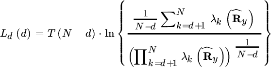
The statistical criterion for model order selection is a classification problem among N possible choices (Section 23.2), and it is based on the likelihood ratio between two alternative hypotheses on the eigenvalues ![]() . By setting d as the test variable, the hypothesis that the
. By setting d as the test variable, the hypothesis that the ![]() smallest eigenvalues are equal is compared with the other hypothesis that
smallest eigenvalues are equal is compared with the other hypothesis that ![]() of the smallest are equal. A sufficient statistic is the ratio between the arithmetic and the geometric mean [69]
of the smallest are equal. A sufficient statistic is the ratio between the arithmetic and the geometric mean [69]
and when ![]() eigenvalues are all equal,
eigenvalues are all equal, ![]() .
.
Other approaches add to the metric Ld(d) a penalty function related to the degrees of freedom
and the model order is the minimizer of this new metric. Using the information‐theoretic criterion there are two main methods:
- Akaike Information Criterion (AIC) test [70]

- Minimum Description Length (MDL) test [71]
so that the model order is the argument that minimizes one of these two criteria as being the order that matches the degrees of freedom of the sample covariance ![]() , which is representative of the dimension of the signal subspace in the frequency estimation problem. The MDL estimate dMDL is consistent and for
, which is representative of the dimension of the signal subspace in the frequency estimation problem. The MDL estimate dMDL is consistent and for ![]() with
with ![]() ; while AIC is inconsistent and tends to overestimate the model order. However, for a small number of measurements T, the AIC criterion is to be preferred.
; while AIC is inconsistent and tends to overestimate the model order. However, for a small number of measurements T, the AIC criterion is to be preferred.