
17
Equalization in Communication Engineering
Deconvolution (Section 5.2.3 and Section 10.1) is the linear filter that compensates for a waveform distortion of convolution. In communication systems, equalization refers to the compensation of the convolutive mixing due to the signals’ propagation (in this context it is called the communication channel), either in wireless or wired digital communications. Obviously, deconvolution is the same as equalization, even if it is somewhat more general as being independent of the specific communication system setup. In MIMO systems (Section 5.3) there are multiple simultaneous signals that are propagating from dislocated sources and cross‐interfering; the equalization should separate them (source separation) and possibly compensate for the temporal/spatial‐channel convolution. The focus of this chapter is to tailor the basic estimation methods developed so far to the communication systems where single or multiple channels are modeled as time‐varying, possibly random with some degree of correlation. Signals are drawn from a finite alphabet of messages and are thus non‐Gaussian by nature [57] . To limit the contribution herein to equalization methods, the estimation of the communication channel (or channel identification, see Section 5.2.3) is not considered as being estimation in a linear model with a known excitation. In common communication systems, channel estimation is part of the alternate communication of a training signal interleaved with the signal of interest as described in Section 15.2. There are blind‐estimation methods that can estimate the channel without a deterministic knowledge of transmitted signals, relying only on their non‐Gaussian nature. However, blind methods have been proved to be too slow in convergence to cope with time‐variation in real systems and thus of low practical interest for most of the communication engineering community.
17.1 Linear Equalization
In linear modulation, the transmitted messages are generated by scaling the same waveform for the corresponding information message that belongs to a finite set of values (or alphabet) ![]() with cardinality
with cardinality ![]() that depends on symbol mapping (Section 15.2). It is common to consider a multi‐level modulation with
that depends on symbol mapping (Section 15.2). It is common to consider a multi‐level modulation with ![]() , or
, or ![]() if complex valued. The transmitted signal is received after convolution by the channel and symbol‐spaced sampling that is modeled as (see Section 15.2):
if complex valued. The transmitted signal is received after convolution by the channel and symbol‐spaced sampling that is modeled as (see Section 15.2):
with ![]() and white Gaussian noise
and white Gaussian noise
Linear equalization (Figure 17.1) needs to compensate for the channel distortion by an appropriate linear filtering ![]() as
as
so that the equalization error
is small enough, and the equalized signal coincides with the undistorted transmitted one up to a certain degree of accuracy granted by the equalizer.
![Communication system model displaying 2 boxes labeled channel H(z) and equalization G(z) with a crossed circle in between, and with connecting arrows labeled a[n], w[n], x[n], and aˆ[n].](http://images-20200215.ebookreading.net/9/3/3/9781119293972/9781119293972__statistical-signal-processing__9781119293972__images__c17f001.gif)
Figure 17.1 Communication system model: channel H(z) and equalization G(z).
Inspection of the error highlights two terms:

The first is the noise filtered by the equalizer g[n], and the second one is the incomplete cancellation of the channel distortions. Design of linear equalizers as linear estimators of a[n] have been already discussed as deconvolution (Section 12.2); below is a review using the communication engineering jargon. In digital communications, the symbols a[n] are modeled as a stochastic WSS process that is multivalued and non‐Gaussian; samples are zero‐mean and independent and identically distributed (iid):
and the autocorrelation sequence is
There are two main criteria adopted for equalization based on which the error of (17.1) is accounted for in optimization.
17.1.1 Zero Forcing (ZF) Equalizer
The zero‐forcing (ZF) equalizer is
called this way as it nullifies any residual channel distortion: ![]() . The benefit is the simplicity but the drawbacks are the uncontrolled amplification of the noise that is filtered by the equalizer with error
. The benefit is the simplicity but the drawbacks are the uncontrolled amplification of the noise that is filtered by the equalizer with error ![]() (e.g., any close to zero H(ω) enhances uncontrollably the noise as
(e.g., any close to zero H(ω) enhances uncontrollably the noise as ![]() ), and the complexity in filter design that could contain causal/anti‐causal responses over an infinite range.
), and the complexity in filter design that could contain causal/anti‐causal responses over an infinite range.
17.1.2 Minimum Mean Square Error (MMSE) Equalizer
The minimization of the overall error ![]() accounts for both noise and residual channel distortion. The z‐transform of the autocorrelation of the error:
accounts for both noise and residual channel distortion. The z‐transform of the autocorrelation of the error:
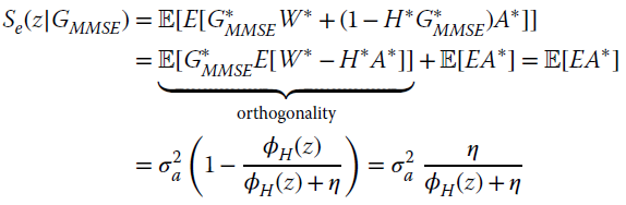
depends on filter response {g[n]}. The minimization of ![]() wrt the equalizer yields to the orthogonality condition as for the Wiener filter (Section 12.2):
wrt the equalizer yields to the orthogonality condition as for the Wiener filter (Section 12.2):
and the (linear) MMSE equalizer is
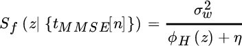
The MMSE equalizer converges to

for the two extreme situations of small or large noise, respectively and ![]() is called matched filter as it acts as a filter that correlates exactly with H(z). Needless to say, linear MMSE is sub‐optimal and some degree of non‐linearity that accounts for the alphabet
is called matched filter as it acts as a filter that correlates exactly with H(z). Needless to say, linear MMSE is sub‐optimal and some degree of non‐linearity that accounts for the alphabet ![]() is necessary to attain the performance of a true MMSE equalizer.
is necessary to attain the performance of a true MMSE equalizer.
17.1.3 Finite‐Length/Finite‐Block Equalizer
This is the convolution of a finite block of symbols a with the finite length channel h, and its equalization is
The equalization using the ZF condition seeks for
and the MMSE
To solve these minimizations, one has to replace the notation with the convolution matrix for the channel h as in Section 5.2 and Section 5.2.3. The optimizations reduce to the one for MIMO systems and solutions are detailed below in Section 17.3.
17.2 Non‐Linear Equalization
Given the statistical properties of signals, the optimal Bayesian estimator is non‐linear and resembles the one derived in Section 11.1.3. However, some clever reasoning can simplify the complexity of non‐linear Bayesian estimator by the so called Decision Feedback Equalization (DFE). The channel response ![]() contains causal (post‐cursor) and anti‐causal (pre‐cursor) terms, and the DFE exploits the a‐priori information on the finite alphabet
contains causal (post‐cursor) and anti‐causal (pre‐cursor) terms, and the DFE exploits the a‐priori information on the finite alphabet ![]() for some temporary linear estimates based on the causal part of h[n]. The approximation of the Bayesian estimator is to use the past to predict the current degree of self‐interference for its reduction, after these temporary estimates are mapped onto the finite alphabet
for some temporary linear estimates based on the causal part of h[n]. The approximation of the Bayesian estimator is to use the past to predict the current degree of self‐interference for its reduction, after these temporary estimates are mapped onto the finite alphabet ![]() .
.
Referring to the block diagram in Figure 17.2, the equalizer is based onto two filters C(z) and D(z), and one mapper onto the alphabet ![]() (decision). The decision is a non‐linear transformation that maps the residual onto the nearest‐level of the alphabet (see Figure 17.3 for
(decision). The decision is a non‐linear transformation that maps the residual onto the nearest‐level of the alphabet (see Figure 17.3 for ![]() ). The filter C(z) is designed based on the ZF or MMSE criteria, and the filter
). The filter C(z) is designed based on the ZF or MMSE criteria, and the filter ![]() is strictly causal as it uses all the past samples in attempt to cancel the contribution of the past onto the current sample value and leave ɛ[n] for decisions. When the decision â[n] is correct, the cancellation reduces the effect of the tails of the channel response but when noise is too large, the decisions could be wrong and these errors accumulate; the estimation is worse than linear equalizers. This is not surprising as the detector replaces a Bayes estimator with a sharp piecewise non‐linearity in place of a smooth one, even when the noise is large (see Section 11.1.3). Overall, the DFE reduces to the design of two filters.
is strictly causal as it uses all the past samples in attempt to cancel the contribution of the past onto the current sample value and leave ɛ[n] for decisions. When the decision â[n] is correct, the cancellation reduces the effect of the tails of the channel response but when noise is too large, the decisions could be wrong and these errors accumulate; the estimation is worse than linear equalizers. This is not surprising as the detector replaces a Bayes estimator with a sharp piecewise non‐linearity in place of a smooth one, even when the noise is large (see Section 11.1.3). Overall, the DFE reduces to the design of two filters.
![Flow diagram of decision feedback equalization displaying 5 boxes labeled H(z), T(z), 1 +D(z), and D(z), 2 crossed circles, and connecting arrows labeled a[n], w[n], x[n], f [n], etc.](http://images-20200215.ebookreading.net/9/3/3/9781119293972/9781119293972__statistical-signal-processing__9781119293972__images__c17f002.gif)
Figure 17.2 Decision feedback equalization.
Figure 17.3 Decision levels for  .
.
The filter C(z) is decoupled into two terms
where ![]() acts as a compensation of the feedback filter D(z), and the filters to be designed are T(z) and D(z). Assuming that all decisions are correct
acts as a compensation of the feedback filter D(z), and the filters to be designed are T(z) and D(z). Assuming that all decisions are correct ![]() (almost guaranteed for noise
(almost guaranteed for noise ![]() small enough), the z‐transform of the error
small enough), the z‐transform of the error

contains two terms: the residual of the equalization, and the filtered noise. The design depends on how to account for these two terms.
17.2.1 ZF‐DFE
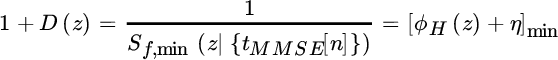
The filter T(z) can be designed to nullify the residual of the filter equalization (zero‐forcing condition); then the design of the causal filter D(z) is a free parameter to minimize the filtered noise. More specifically, the choice is
and the filter D(z) should be chosen to minimize the power of the filtered noise ![]() with power spectral density in z‐transform
with power spectral density in z‐transform
The structure of the filter ![]() is monic and causal, it can be considered as a linear predictor (Section 12.3) for the process f[n] correlated by T(z). The factorization
is monic and causal, it can be considered as a linear predictor (Section 12.3) for the process f[n] correlated by T(z). The factorization ![]() into min/max phase terms according to the Paley–Wiener theorem (Section 4.4.3) (recall that
into min/max phase terms according to the Paley–Wiener theorem (Section 4.4.3) (recall that ![]() but it is not necessarily true that
but it is not necessarily true that ![]() , see Appendix
of Chapter 4) yields to the choice
, see Appendix
of Chapter 4) yields to the choice
Alternatively, and without any change of the estimator, one can make the factorization of the filter into min/max phase ![]() and the filter becomes
and the filter becomes

Filters are not constrained in length, but one can design ![]() using a limited‐length linear predictor at the price of a small performance degradation.
using a limited‐length linear predictor at the price of a small performance degradation.
17.2.2 MMSE–DFE
In the MMSE method, the minimization is over the ensemble of error (17.2). Namely, the error can be rewritten by decoupling the terms due to the filter T(z)
and the linear predictor ![]() as
as
The power spectral density of f[n] depends on t[n]:
and the MMSE solution is from orthogonality, or equivalently the minimization

where ![]() , and
, and ![]() .
.
The linear predictor ![]() follows by replacing the terms. The (minimal) PSD for the filter
follows by replacing the terms. The (minimal) PSD for the filter ![]() is
is
and its min/max phase factorization defines the predictor
The filter C(z) for the MMSE–DFE equalizer is

which is a filter with causal/anti‐causal component.
Remark. Since the filter’s length is unbounded and can have long tails, the implementation of the MMSE–DFE could be quite expensive in terms of computations. A rule of thumb is to smoothly truncate the response cMMSE[n] by a window over an interval that is in the order of 4–6 times the length of the channel h[n]. In other cases, the design could account for the limited filter length with better performance compared to a plain truncation, even if smooth.
17.2.3 Finite‐Length MMSE–DFE
The MMSE–DFE can be designed by constraining the length of the filters to be limited [75] . Making reference to Figure 17.4, the ![]() filter c can have a causal and anti‐causal component so that
filter c can have a causal and anti‐causal component so that

where the last equality is for correct decisions, and ![]() . The error
. The error
is represented in terms of the augmented terms ![]() and
and ![]() , and the MSE becomes
, and the MSE becomes
Figure 17.4 Finite length MMSE–DFE.
The optimization wrt c for known d (the constraint condition is usually added at last step) is quadratic:
and the MSE
is a quadratic form, but the constraint condition ![]() has not been used yet.
has not been used yet.
Rewriting explicitly the MSE (17.3)
after partitioning

it yields the solution
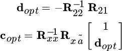
and the MSE for this optimized solution becomes ![]() .
.
In the case that the channel has length Nh samples, the empirical rules are

with ![]() . However, since the optimal MSE has a closed form, the filters’ length can be optimized for the best (minimum) MSEmin within a predefined set; this is the preferred solution whenever this is practicable.
. However, since the optimal MSE has a closed form, the filters’ length can be optimized for the best (minimum) MSEmin within a predefined set; this is the preferred solution whenever this is practicable.
17.2.4 Asymptotic Performance for Infinite‐Length Equalizers
The performance is evaluated in terms of MSE. For a linear MMSE equalizer, the MSE is

where ![]() , and by using the solutions derived above (argument z is omitted in z‐transforms)
, and by using the solutions derived above (argument z is omitted in z‐transforms)
it is

The steps for the MMSE–DEF equalizer are the same as above by replacing the solutions for the ![]() and after some algebra [74] :
and after some algebra [74] :

Since
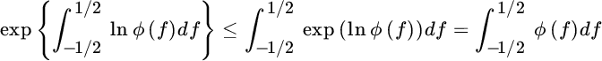
according to the Jensen inequality for convex transformation exp(.) (Section 3.2) for  this proves that
The DFE should always be preferred to the linear MMSE equalizer except when noise is too large to accumulate errors.
17.3 MIMO Linear Equalization
MIMO refers to linear systems with multiple input/output as discussed in model definition in Section 5.3, a block of N symbols a are filtered by an ![]() matrix H with
matrix H with ![]() (i.e., more receivers that transmitted symbols) and received signals are
(i.e., more receivers that transmitted symbols) and received signals are
with noise ![]() . MIMO equalization (Figure 17.5) refers to the linear or non‐linear procedures to estimate a from x provided that H is known. In some contexts the interference reduction of the equalization is referred as MIMO decoding if the procedures are applied to x, and MIMO precoding if applied to a before being transmitted as transformation g(a) with model
. MIMO equalization (Figure 17.5) refers to the linear or non‐linear procedures to estimate a from x provided that H is known. In some contexts the interference reduction of the equalization is referred as MIMO decoding if the procedures are applied to x, and MIMO precoding if applied to a before being transmitted as transformation g(a) with model ![]() , possibly linear
, possibly linear ![]() . The processing variants for MIMO systems are very broad and are challenging many researchers in seeking different degrees of optimality. The interested reader might start from [72,73].
. The processing variants for MIMO systems are very broad and are challenging many researchers in seeking different degrees of optimality. The interested reader might start from [72,73].

Figure 17.5 Linear MIMO equalization.
To complete the overview, the model (17.4) describes the block (or packet‐wise) equalization when a block of N symbols a are arranged in a packet filtered with a channel of ![]() samples, and the overall range is
samples, and the overall range is ![]() ; the matrix H in (17.4) is the convolution matrix in block processing.
; the matrix H in (17.4) is the convolution matrix in block processing.
17.3.1 ZF MIMO Equalization
Block linear equalization is based on a transformation ![]() such that the ZF condition holds:
such that the ZF condition holds: ![]() . The estimate is
. The estimate is
and the metric to be optimized is the norm of the filtered noise ![]() . The optimization is constrained as
. The optimization is constrained as
to be solved by the Lagrange multiplier method by augmenting the metric with N2 constraints using the ![]() matrix
matrix ![]() :
:
Optimization wrt G is (Section 1.8 and Section 1.8.2)
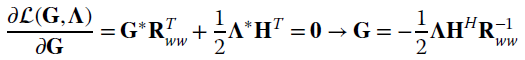
using the constraint condition

it yields the ZF equalization
Note that the ZF solution can be revised as follows. Since ![]() , the Cholesky factorization
, the Cholesky factorization ![]() into lower/upper triangular matrixes is unique, and similarly
into lower/upper triangular matrixes is unique, and similarly ![]() . The ZF estimate is
. The ZF estimate is
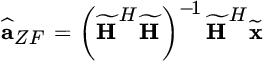
where ![]() and
and ![]() ; it can be interpreted as the pseudoinverse of
; it can be interpreted as the pseudoinverse of ![]() for the pre‐whitened observation
for the pre‐whitened observation ![]() .
.
17.3.2 MMSE MIMO Equalization
The linear MMSE estimator has already been derived in many contexts. To ease another interpretation, the estimator is the minimization of the MSE
for the symbols with correlation ![]() . The MMSE solution follows from the orthogonality (Section 11.2.2)
. The MMSE solution follows from the orthogonality (Section 11.2.2)
This degenerates into the ZF for large signals (or ![]() ) as
) as ![]() ; and for large noise it becomes
; and for large noise it becomes ![]() . The MSE for âMMSE can be evaluated after the substitutions.
. The MSE for âMMSE can be evaluated after the substitutions.
17.4 MIMO–DFE Equalization
The MIMO–DFE in Figure 17.6 is just another way to implement the cancellation of interference embedded into MIMO equalization, except that the DFE cancels the interference from decisions—possibly the correct ones. In MIMO systems this is obtained from the ordered cancellation of samples, where the ordering is a degree of freedom that does not show up in equalization as in these systems, samples are naturally ordered by time. Before considering the DFE, it is essential to gain insight into analytical tools to establish the equivalence between DFE equalization and its MIMO counterpart.
Figure 17.6 MIMO–DEF equalization.
17.4.1 Cholesky Factorization and Min/Max Phase Decomposition
The key algebraic tool for MIMO–DFE is the Cholesky factorization that transforms any ![]() into the product of two triangular matrixes, one the Hermitian transpose of the other—sometimes referred as the (unique) square‐root of R:
into the product of two triangular matrixes, one the Hermitian transpose of the other—sometimes referred as the (unique) square‐root of R:
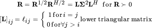
where the entries of the diagonal matrix ![]() are all positive. For zero‐mean rvs, Cholesky factorization of the correlation matrix is the counterpart of min/max phase decomposition of the autocorrelation sequence. To prove this, let
are all positive. For zero‐mean rvs, Cholesky factorization of the correlation matrix is the counterpart of min/max phase decomposition of the autocorrelation sequence. To prove this, let ![]() be an
be an ![]() vector with covariance
vector with covariance ![]() . Transformation by a lower triangular matrix L with normalized terms along the diagonal is
. Transformation by a lower triangular matrix L with normalized terms along the diagonal is

and the covariance is
If it is now assumed that a vector y has covariance ![]() , the transformation can be inverted as
, the transformation can be inverted as ![]() —still lower triangular (
—still lower triangular (![]() for
for ![]() ). The i th entry is
). The i th entry is

where ![]() extracts the i th row from
extracts the i th row from ![]() . Since
. Since ![]() and
and ![]() then
then ![]() is a linear predictor that uses all the samples
is a linear predictor that uses all the samples ![]() (similar to a causal predictor over a limited set of samples) to estimate yi, and
(similar to a causal predictor over a limited set of samples) to estimate yi, and ![]() is the variance of the prediction error. If choosing
is the variance of the prediction error. If choosing ![]() the linear predictor makes use of the complementary samples
the linear predictor makes use of the complementary samples ![]() to estimate yi and the predictor would be reversed (anti‐causal). For a WSS random process, the autocorrelation can be factorized into the convolution of min/max phase sequences, and these coincide with the Cholesky factorization of the Toeplitz structured correlation matrix R for
to estimate yi and the predictor would be reversed (anti‐causal). For a WSS random process, the autocorrelation can be factorized into the convolution of min/max phase sequences, and these coincide with the Cholesky factorization of the Toeplitz structured correlation matrix R for ![]() . However when N is small, the Cholesky factorization of the correlation matrix R takes the boundary effects into account, and the predictors (i.e., the rows of
. However when N is small, the Cholesky factorization of the correlation matrix R takes the boundary effects into account, and the predictors (i.e., the rows of ![]() ) are not just the same shifted copy for every entry.
) are not just the same shifted copy for every entry.
17.4.2 MIMO–DFE
In MIMO–DFE, the received signal x is filtered by a compound filter to yield
where the normalized (![]() for
for ![]() ) lower triangular matrix L is decoupled into the strictly lower triangular B and the identity I to resemble the same structure as DFE in Section 17.2. The matrix DFE acts sequentially on decisions as the product
) lower triangular matrix L is decoupled into the strictly lower triangular B and the identity I to resemble the same structure as DFE in Section 17.2. The matrix DFE acts sequentially on decisions as the product

isolates the contributions and Bâ sequentially orders the contributions arising from the upper lines toward the current one: ![]() . The fundamental equation of DFE is the equality of the decision variable from the previous decisions carried out from the upper lines:
. The fundamental equation of DFE is the equality of the decision variable from the previous decisions carried out from the upper lines:
From the partition above:
according to the model
There are two metrics to be optimized based on the double constraint on the structure of L according to the ZF or MMSE constraint:

For both criteria the second step, which is based on the first solution, is peculiar for DFE and it implies the optimization of a metric with the constraint on the normalized lower triangular structure of the matrix L. Namely, in both cases it follows the minimization
for a certain positive definite matrix ![]() that is, for the two cases and
that is, for the two cases and ![]() :
:
Since ![]() , its Cholesky factorization, is
, its Cholesky factorization, is
where ![]() with
with ![]() . On choosing
. On choosing
it follows that
Solutions for AWGN ![]() are derived below.
are derived below.
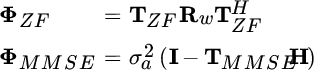
ZF–DFE for AWGN: 
The optimization
yields the same solution as in Section 17.3.1:
Since the noise after filtering TZF is ![]() , the metric of (17.5) becomes
, the metric of (17.5) becomes ![]() and the filter LZF follows from its Cholesky factorization
and the filter LZF follows from its Cholesky factorization
MMSE–DFE for AWGN: 
The solution of the first term is straightforward from orthogonality (or the MMSE–MIMO solution):

using here any of the two equivalent representations (Section 11.2.2), with ![]() . The matrix
. The matrix  , where the second equality follows from the matrix inversion lemma (Section 1.1.1), and LMMSE is from the Cholesky factorization.