
14
Spectral Analysis
In time series analysis, the estimation of the correlation properties of random samples is referred to as spectral analysis. If a process x[n] is stationary, its correlation properties are fully defined by the autocorrelation or equivalently by its Fourier transform, in term of power spectral density (PSD):
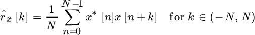
Spectral analysis deals with the estimation of a PSD from a limited set of N observations ![]() :
:
There are two fundamental approaches to spectral analysis: parametric or non‐parametric, depending if there is a parametric model for the PSD or not. Non‐parametric spectral analysis makes no assumptions on the PSD and thus it is more general and flexible as it can be used in every situation when there is no a‐priori knowledge on the mechanism that correlates the samples in the time series. Parametric methods model (or guess) the generation mechanism of the process and thus the spectral analysis reduces to the estimate of these parameters. Except for a few cases, spectral analysis is basically a search for the most appropriate (non‐parametric/parametric) method to better estimate the PSD and some features that are of primary interest for the application.
There is no general rule to carrying out spectral analysis except for common sense related to the needs of the specific application. Therefore, the organization of this chapter aims to offer a set of tools and to establish the pros and cons of each method based on statistical performance metrics. The lack of a general method that is optimal for every application makes spectral analysis a professional expertise itself where experience particularly matters. For this reason, spectral analysis is considered “an art”, and the experts are “artisans” of spectral analysis who specialize in different application areas. All the principal methods are discussed herein with the usual pragmatic approach aiming to provide the main tools to deal with the most common problems and to refine the intuition, while avoiding entering into excessive detail in an area that could easily fill a whole dedicated book, see e.g., [52].
14.1 Periodogram
Spectral analysis estimates the PSD ![]() from the observations
from the observations ![]() , and performance is evaluated by the bias
, and performance is evaluated by the bias ![]() and the variance
and the variance ![]() . As for any estimator, it is desirable that the PSD estimate is unbiased (at least asymptotically as
. As for any estimator, it is desirable that the PSD estimate is unbiased (at least asymptotically as ![]() ) and consistent. Non‐parametric spectral analysis is the periodogram, and it is historically based on the concept of the filter‐bank revised in Section 14.1.3, as every value of the PSD represents the power collected by a band‐pass filter centered at the specific frequency bin.
) and consistent. Non‐parametric spectral analysis is the periodogram, and it is historically based on the concept of the filter‐bank revised in Section 14.1.3, as every value of the PSD represents the power collected by a band‐pass filter centered at the specific frequency bin.
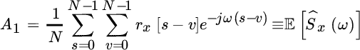
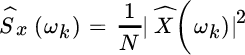
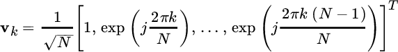
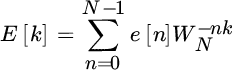
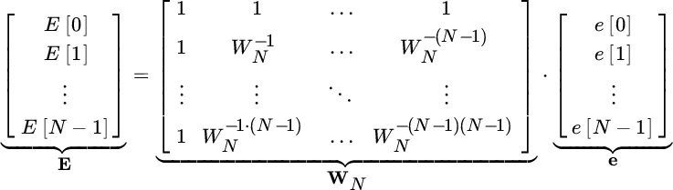
Let

be the discrete Fourier transform (DFT) of the sequence x evaluated for the k th bin of the angular frequency ![]() (or k th frequency bin
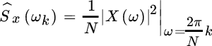
(or k th frequency bin ![]() ). The periodogram is the estimator
). The periodogram is the estimator
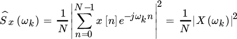
and it corresponds to the energy density of the sequence of N samples |X(ωk)|2 divided by the number of samples. If considering unit‐time sampling, the periodogram divides the energy density by the observation time and reflects the definition of power density (power per unit of frequency bin). The periodogram has the benefit of simplicity and computational efficiency and this motivates its widespread use. However, an in‐depth knowledge of its performance is mandatory in order to establish the limits of this simple and widely adopted estimator.
14.1.1 Bias of the Periodogram
A careful inspection of the definition of the periodogram shows that the periodogram can be rewritten as an FT of the sequence of N samples ![]() sampled in regular frequency bins:
sampled in regular frequency bins:
but
is the FT of the sample autocorrelation
The properties of ![]() govern the bias, and since (see Appendix A)
govern the bias, and since (see Appendix A)

this proves that the periodogram (a sampled version of ![]() ) is biased, as
) is biased, as

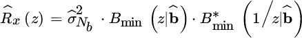
where the convolution ![]() is periodic over 2π. The periodgram is a biased estimator of the PSD that is asymptotically unbiased as
is periodic over 2π. The periodgram is a biased estimator of the PSD that is asymptotically unbiased as

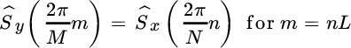
Remark 1: The properties of the DFT makes it possible to evaluate the FT in other frequency bins, not necessarily spaced by 1/N (or 2π/N if angular frequency bins). This is obtained by padding with zeros the sequence ![]() up to a new value, say
up to a new value, say ![]() :
:
From signal theory [12,13] , the DFT over the M samples is the FT of the sequence sampled over the new frequency bin, which in turn is correlated (i.e., not statistically independent or uncorrelated) with the DFT X(ωk):

The DFT of y[n] is the interpolated values of DFT of x[n] (14.1) using the periodic sinc as interpolating function.
A common practice is to pad to multiple values of N, say ![]() , so that the interpolating function
, so that the interpolating function ![]() ) honors the DFT X(ωk) and thus the periodogram
) honors the DFT X(ωk) and thus the periodogram ![]() coincides with
coincides with ![]() as
as
with ![]() interpolated values between the samples of the
interpolated values between the samples of the ![]() .
.
Remark 2: The bias (14.3) vanishes when considering some special cases. Let the PSD of one (or more) real (or complex) sinusoids with amplitude A, random phase, and frequency ωo be
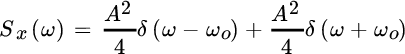
The bias becomes
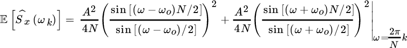
and the periodogram is biased as shown in Figure 14.1. However, if the frequency
for some integer value ℓo (i.e., the sinusoid has a period that makes ℓo cycles into the N samples of the observation window), the periodogram is unbiased, as

Since the value of periodogram in ℓo is ![]() , apparently the periodogram seems to yield a wrong value for the power of the sinusoid, as it should be A2/2. Recall that the periodogram is the estimator of the power spectrum “density” and thus the power is obtained by multiplying each bin by the corresponding bandwidth, which in this case it is the frequency bin spacing 1/N, and thus
, apparently the periodogram seems to yield a wrong value for the power of the sinusoid, as it should be A2/2. Recall that the periodogram is the estimator of the power spectrum “density” and thus the power is obtained by multiplying each bin by the corresponding bandwidth, which in this case it is the frequency bin spacing 1/N, and thus
as expected
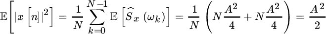
Another interesting case is when the PSD is for a white WSS random process:
when the bias becomes
that is, still unbiased. Once again, the power is still the same as summing N terms scaled by the bandwidth 1/N of the periodogram bin; the power is ![]()
![]() .
.
Figure 14.1 Bias of periodogram for sinusoids.
14.1.2 Variance of the Periodogram
The exact evaluation of the variance of the periodogram is not straightforward, but some simplifications in the simple case can be drawn before providing the general equation. For a real‐valued process, it can be written as

The computation needs the 4th order moments, which are not straightforward. However, the computation becomes manageable if the process is Gaussian and white (in this way all the conclusions can be extended to every bin, regardless of the bias effect in (14.3)) so that ![]() . For stationary processes involving stationarity up to the 4th order moment of the Gaussian process (this condition is stricter than wide‐sense stationary condition, but not uncommonly seen to be fulfilled):1
. For stationary processes involving stationarity up to the 4th order moment of the Gaussian process (this condition is stricter than wide‐sense stationary condition, but not uncommonly seen to be fulfilled):1

and furthermore from the bias:

These two identities let us simplify the variance (14.4) as

and the first term can be further simplified from (14.5) into the sum of two terms that from complex conjugate symmetry are

The first term becomes (from (14.5))
while the second term can be evaluated in closed form from the statistical uncorrelation of the samples

To summarize, the variance of the periodogram for an observation of N samples of a white Gaussian process with power ![]() is
is
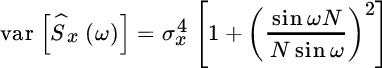
and for the samples of the periodogram it is

The periodogram is not consistent as its variance does not vanish for ![]() and some remedies are mandatory in order to use the periodogram as a PSD estimator, since in this simple form the variance of the periodogram is intolerably high and, surprisingly, it is a very bad estimator!
and some remedies are mandatory in order to use the periodogram as a PSD estimator, since in this simple form the variance of the periodogram is intolerably high and, surprisingly, it is a very bad estimator!
The variance derived so far can be used as a good approximation for the variance in any context (not necessarily for white Gaussian processes), and it follows the routinely adopted variance of the periodogram for real‐valued discrete‐time signals:

without the effect of bias. Control of the variance is mandatory in order to use the periodogram effectively as an estimator of the PSD, and this will be discussed next.
Remark: The periodogram is based on the DFT and thus all the properties of symmetry of Fourier transforms hold. Namely, if the process is real, ![]() , and this motivates the larger variance for the samples
, and this motivates the larger variance for the samples ![]() . However, for a complex process the DFT is no longer symmetric:
. However, for a complex process the DFT is no longer symmetric: ![]() , and the variance is the same for all frequency bins:
, and the variance is the same for all frequency bins:
A justification is offered in the next section.
14.1.3 Filterbank Interpretation
The relationship (14.6) is not surprising if one considers the effective measurements carried out by every frequency bin. The periodogram can be interpreted as a collection of signals from an array of band‐pass filters (filter‐bank) that separates the signal x[n] into the components ![]() such that (Figure 14.2)
such that (Figure 14.2)
where the kth filter is centered at the frequency ![]() with a bandwidth
with a bandwidth ![]() to guarantee a uniform filter‐bank (see [55] for multirate filtering and filter‐banks).
to guarantee a uniform filter‐bank (see [55] for multirate filtering and filter‐banks).
The samples yk[n] are temporally correlated as the bandwidth of the process is as wide as the bandwidth of the filter Hk(ω); these samples can be extracted with a coarser sampling rate that extracts one sample every N (decimation 1:N) so that the samples after the filter‐bank are a set of components ![]() ; these components are statistically uncorrelated (as maximally decimated [55]) and can be used to extract the power of each component
; these components are statistically uncorrelated (as maximally decimated [55]) and can be used to extract the power of each component
as estimate of the corresponding power. Since the samples are random
it follows that2
thus showing that the power from every filter is the estimate of the PSD with variance S2(ωk). The filter‐bank is not just a model, but it coincides with the periodogram where the filter‐bank implements the DFT as in Figure 14.2 and the filters are chosen as

This gives an interesting interpretation to the bias of the periodogram as being due to the poor selectivity of the band‐pass filtering, which can be significantly improved by choosing a different filter response as discussed below in Section 14.1.5.
Figure 14.2 Filter‐bank model of periodogram.
14.1.4 Pdf of the Periodogram (White Gaussian Process)
As the periodogram is an rv that in every cell estimates the corresponding PSD, in order to gain insight, it is useful to evaluate the corresponding pdf for the same context of Section 14.1.2. Let the data be
The DFT that is a linear transformation of x (see Remark 3 of Appendix B)

so that highlighting the bins X[0 : N/2] as statistically independent, we have:
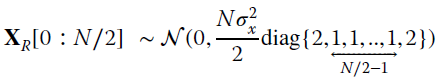

or equivalently
Each bin of the periodogram is the square of the DFT so that
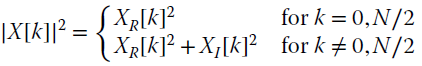
which is the sum of the square of two independent and Gaussian rvs, and the pdf is exponential (central Chi‐Square ![]() with 2 degrees of freedom):
with 2 degrees of freedom):
with rate parameter ![]() . From the properties of the exponential pdf:
. From the properties of the exponential pdf:

where we included the results for ![]() . Using the definition of the periodogram (14.2), all results derived so far should be scaled by 1/N and this coincides with Section 14.1.2.
. Using the definition of the periodogram (14.2), all results derived so far should be scaled by 1/N and this coincides with Section 14.1.2.
For the case
(there is no correlation between X[k] and ![]() as for real valued processes) and thus
as for real valued processes) and thus

that is, there is no difference for the variance among samples of the periodogram.
14.1.5 Bias and Resolution
The periodogram is biased, and the total bias depends on the length N. The main consequences of bias is loss of resolution,3 smoothing of the PSD, and spectral leakage due to the side‐lobes of the biasing periodic sinc(.) function in (14.3). To gain insight into this, consider the periodogram to estimate the PSD in the case of a selective PSD as in Figure 14.3. In bias (14.3) the periodic sinc

that governs the convolution with the PSD Sx(ω) can be divided into two terms over disjoint intervals (i.e., ![]() ): the main lobe BP(ω) over the interval
): the main lobe BP(ω) over the interval ![]() and the side‐lobes BL(ω):
and the side‐lobes BL(ω):
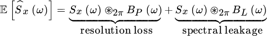
as sketched in Figure 14.3. The main lobe has the effect of smoothing the PSD in the case Sx(ω) as a rapid transition with a loss of selectivity and resolution as illustrated when evaluating ![]() (solid line) compared to the PSD Sx(ω) (dashed line). The side‐lobes have the effect of spreading the PSD over the frequency axis where the PSD Sx(ω) is very small (spectral leakage), thus creating artifacts such as
(solid line) compared to the PSD Sx(ω) (dashed line). The side‐lobes have the effect of spreading the PSD over the frequency axis where the PSD Sx(ω) is very small (spectral leakage), thus creating artifacts such as ![]() that are not in the PSD. The overall effect is a “distorted” PSD (solid line) that in some cases can be unacceptable.
that are not in the PSD. The overall effect is a “distorted” PSD (solid line) that in some cases can be unacceptable.
A detailed inspection of the reasons for bias proves that it is a consequence of the abrupt (rectangular‐like) truncation of the data that can be mitigated by a smooth windowing. Re‐interpreting the periodogram
as the DFT of the samples
obtained after the rectangular windowing w[n] (that is, ![]() for
for ![]() ) gives the interpretation of the bias as the consequence of the truncation. Any arbitrary window w[n] on the data x[n] before DFT affects the autocorrelation, as if the windowing is
) gives the interpretation of the bias as the consequence of the truncation. Any arbitrary window w[n] on the data x[n] before DFT affects the autocorrelation, as if the windowing is ![]() , and the bias is
, and the bias is
which is to be evaluated for ![]() . The window w[n] can be smooth to reduce the side‐lobes of the corresponding Fourier transform, and thus it mitigates spectral leakage. However, this is at the expense of a loss of resolution, as windows with small side‐lobes have a broader main lobe. The Figure 14.4 shows an example of the most common windows and their Fourier transforms; the choice of the data‐windowing is a trade‐off between resolution and spectral leakage. Needless to say that windowing changes the total power of the data as the size of the effective data is smaller (edge samples are down weighted), and compensation is necessary to recover the values of the PSD. One side effect of the windowing is the increased variance due to the reduction of the effective data length.
. The window w[n] can be smooth to reduce the side‐lobes of the corresponding Fourier transform, and thus it mitigates spectral leakage. However, this is at the expense of a loss of resolution, as windows with small side‐lobes have a broader main lobe. The Figure 14.4 shows an example of the most common windows and their Fourier transforms; the choice of the data‐windowing is a trade‐off between resolution and spectral leakage. Needless to say that windowing changes the total power of the data as the size of the effective data is smaller (edge samples are down weighted), and compensation is necessary to recover the values of the PSD. One side effect of the windowing is the increased variance due to the reduction of the effective data length.
Figure 14.3 Bias and spectral leakage.
Figure 14.4 Rectangular, Bartlett (or triangular) and Hanning windows w[m] with M = 31, and their Fourier transforms  on frequency axis ω/2π.
14.1.6 Variance Reduction and WOSA
The variance of the periodogram is intolerably high and it prevents its reliable use as a PSD estimator. A simple method for variance reduction is by averaging independent simple periodograms to reduce the variance accordingly (see the examples in Section 6.7). The WOSA method (window overlap spectral analysis) is based on averaging of the periodograms after the segmentation of the data into smaller segments, with some overlap if windowing is adopted (to control the bias as discussed above).
The overall observations can be segmented into M blocks of N samples each as in Figure 14.5. The periodogram is the average of M simple periodograms over N samples:

with a requirement for ![]() observations in place of N. The variance is
observations in place of N. The variance is
and the choice of M can control the accuracy that is needed for the specific application. In practice, the overall observations Ntot are given and the choice of M and N is a trade‐off between the need to have small variance (with M large) and small bias (with N large). Since resolution and spectral leakage can be also controlled by data‐windowing, the overall data can be windowed before computing the simple periodogram. As mentioned in the previous section, the windowing reduces the effective data used, and some overlapping can be tolerated to guarantee that the averaging is for independent periodograms. In WOSA (see Figure 14.6) the overlapping factor
highlights the degree of overlapping in the windowed segmentation, and for a total set of samples Ntot the WOSA periodogram becomes

where the number of overlapping windows is
Once again, the choice of η should guarantee the averaging of independent periodograms. If using a Bartlett window, a reasonable choice is ![]() ; smoothed windows tolerate a larger overlapping η at the price of some spectral leakage.
; smoothed windows tolerate a larger overlapping η at the price of some spectral leakage.

Figure 14.5 Segmentation of data into M disjoint blocks of N samples each.
Figure 14.6 WOSA spectral analysis.
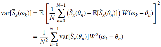
Inspired by the variance mitigation of WOSA with data‐windowing, the variance can be reduced by smoothing a simple periodogram over N samples with a proper smoothing W(ωk) over the whole range of the N samples; this averaging of independent samples is by circular convolution (periodogram smoothing method)

The smoothing function W(ωk) should be positive definite and can be chosen to be rectangular, or triangular (Bartlett shape), or any other shape. Even if the smoothing reduces the variance on the order of the smoothing interval, it introduces a bias that can be seen by the loss of resolution due to the smoothing itself. More specifically, the bias is

where the last approximation is a consequence of the choice of a smoothing window that is large compared to the periodogram spacing 1/N. The choice ![]() guarantees that the smoothing does not add any bias, not even asymptotically. The variance is
guarantees that the smoothing does not add any bias, not even asymptotically. The variance is
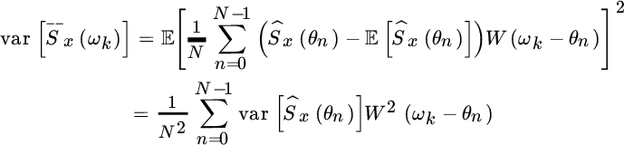
which depends on the variance of the other terms as consequence of the smoothing. Since the influence of the smoothing is to average in the neighborhood of the frequency ωk, it is expected that the PSD is approximately constant within the smoothing window so that the ratio

depends approximately only on the window choice and it can be evaluated for some typical window choices that can be applied either in time (Table 14.1) or as periodogram smoothing in frequency (Table 14.2). Recall that a raised cosine with ![]() is a general window, and it can be specialized to the Hann (or Hanning) window for
is a general window, and it can be specialized to the Hann (or Hanning) window for ![]() , and the Hamming window for
, and the Hamming window for ![]() .
.
Table 14.1 Time windows and variance reduction.
| Time window: w[m] (support
|
 |
| rectangular: |
|
| Bartlett: |
 |
| raised cosine: |
|
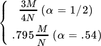 |
Table 14.2 Frequency smoothing and variance reduction.
| Frequency smoothing: W(ωk) |  |
| (support
|
|
| rectangular: |
|
| Bartlett: |
 |
raised cosine:  |
 |
14.1.7 Numerical Example: Bandlimited Process and (Small) Sinusoid
The periodogram is used as the first step in spectral analysis when it would be uncertain to use any parametric method, but bias and variance should be used judiciously. Let us consider as observations
modeled as the sum of a bandlimited process z[n] with bandwidth B and with a small sinusoid superimposed with frequency ![]() close to the edge of the bandlimited process (
close to the edge of the bandlimited process (![]() ). The periodogram is used here to estimate the PSD and highlight the existence, or not, of the sinusoid (intentionally or accidentally) “hidden” on the side of the PSD Sz(f). A numerical analysis can ease the discussion based on the Matlab code below.
). The periodogram is used here to estimate the PSD and highlight the existence, or not, of the sinusoid (intentionally or accidentally) “hidden” on the side of the PSD Sz(f). A numerical analysis can ease the discussion based on the Matlab code below.
The bandlimited process has been generated by filtering a white Gaussian process with a Chebyshev filter that is chosen to have a high order (here 15th order) to guarantee good selectivity with sharp transition between pass‐band and stop‐band; cutoff frequency is chosen as ![]() . The sinusoid has frequency
. The sinusoid has frequency ![]() and amplitude
and amplitude ![]() that is much smaller than the in‐band PSD of Sz(f).
that is much smaller than the in‐band PSD of Sz(f).
The WOSA method has been applied over ![]() segments of
segments of ![]() samples/segment without overlapping by using unwindowed observations (plain periodogram), or by windowing using either Hanning or Bartlett windows. Figure 14.7 shows the superposition of 10 independent simulations of averaged periodograms for different windowing superimposed to the “true” PSD Sz(f) (dashed line). Without windowing, the PSD is biased with a smooth transition toward the edge of the band (f = 1/2) that completely hides the PSD of the sinusoid. A similar conclusion can be drawn for the use of Hanning windowing on the data. On the other hand, the periodogram using Bartlett windows on the observations still has the effect of reducing the selectivity, but this bias does not hide the PSD of the sinusoid and the value of the periodogram at the frequency of the sinusoid restores the true value of the PSD of the sinusoid (filled dot in Figure 14.7).
samples/segment without overlapping by using unwindowed observations (plain periodogram), or by windowing using either Hanning or Bartlett windows. Figure 14.7 shows the superposition of 10 independent simulations of averaged periodograms for different windowing superimposed to the “true” PSD Sz(f) (dashed line). Without windowing, the PSD is biased with a smooth transition toward the edge of the band (f = 1/2) that completely hides the PSD of the sinusoid. A similar conclusion can be drawn for the use of Hanning windowing on the data. On the other hand, the periodogram using Bartlett windows on the observations still has the effect of reducing the selectivity, but this bias does not hide the PSD of the sinusoid and the value of the periodogram at the frequency of the sinusoid restores the true value of the PSD of the sinusoid (filled dot in Figure 14.7).

Figure 14.7 Periodogram (WOSA method) for rectangular, Bartlett, and Hamming window.
The effect of the number of samples is equally important to highlight the sinusoid in the PSD as the periodogram for the sinusoid increases with N (see Section 14.1.5). This is shown in Figure 14.8 where the Bartlett window has been used on observations with increasing length thus showing that N = 128 or 256 samples are not enough to avoid the bias of the periodogram hiding the line spectrum of the sinusoid, while any choice of N = 512 or larger can allow the lines of the sinusoid to exceed the biased PSD of Sz(f).
14.2 Parametric Spectral Analysis
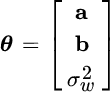
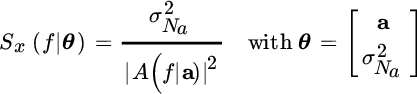
In parametric spectral analysis, the PSD is modeled in terms of a set of parameters θ so that ![]() accounts for the PSD and the estimate of θ yields the estimate of the PSD:
accounts for the PSD and the estimate of θ yields the estimate of the PSD:
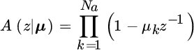
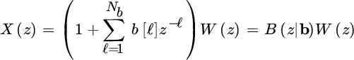
Accuracy depends on the compliance of the parametric model to the PSD of the specific process at hand. To exemplify, if the PSD contains resonances, the parametric model should account for these resonances in a number that is the same as the PSD, otherwise there could be errors due to under‐ or over‐parameterization. Parametric models are based on AR, MA, or ARMA processes (Section 4.4) where the N samples are obtained by properly filtering an uncorrelated Gaussian process w[n] with power (unknown) ![]() . The most general case is the parametric spectral analysis for an ARMA model (ARMA spectral analysis), where the corresponding z‐transform is
. The most general case is the parametric spectral analysis for an ARMA model (ARMA spectral analysis), where the corresponding z‐transform is
![Model for AR spectral analysis, depicted by a rectangle labeled 1/A(ʐ | a) with a rightward arrow at the left labeled w[n] atop and σ2AR(N ₐ) below, and another rightward arrow at the right labeled x[n].](http://images-20200215.ebookreading.net/9/3/3/9781119293972/9781119293972__statistical-signal-processing__9781119293972__images__c14f008.gif)
Figure 14.8 Periodogram (WOSA method) for varying  and Bartlett window.
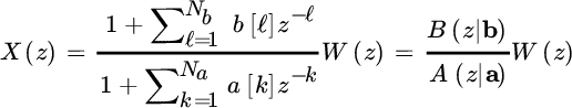
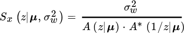
The PSD

is parametric as it depends on the set of ![]() complex‐valued coefficients a and b, and on the power
complex‐valued coefficients a and b, and on the power ![]() acting as a scaling term. The overall parameters
acting as a scaling term. The overall parameters
completely define the PSD, and the model can be reduced to AR (by choosing ![]() ) and MA (by choosing
) and MA (by choosing ![]() ) spectral analysis.
) spectral analysis.
14.2.1 MLE and CRB
The MLE is based on the parametric model of the distribution of x that is based on the Gaussian model:
First of all, it is necessary to evaluate the relationship between the structure of the covariance Cxx and the PSD. Starting from the log‐pdf of the data (see also Section 7.2.4)
each of these terms can be made dependent on the PSD by exploiting the relationships between eigenvalues/eigenvectors of the covariance matrix
and its PSD (Appendix B):

as in spectral analysis a common assumption is to have a large value of N. The k th eigenvector can be approximated by a complex sinusoid with k cycles over N samples:
By substituting into the pdf we get:
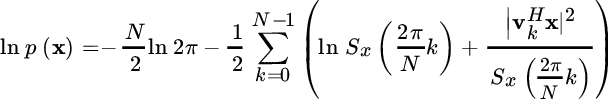
and since ![]() , the term
, the term

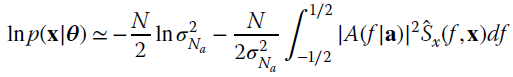
is again the periodogram. The pdf can be rewritten now in terms of the PSD values

Since 1/N is the normalized bandwidth of the frequency bin in the periodogram (recall that ![]() ), the log‐likelihood can be rewritten as
), the log‐likelihood can be rewritten as
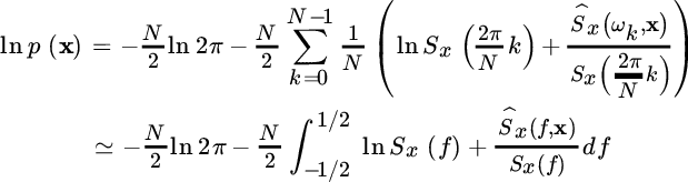
The latter approximation holds for large enough N —in principle for ![]() , and it is the pdf of data for spectral analysis.
, and it is the pdf of data for spectral analysis.
14.2.2 General Model for AR, MA, ARMA Spectral Analysis
For parametric spectral analysis, the PSD ![]() depends on a set of non random parameters θ, so the log‐likelihood is
depends on a set of non random parameters θ, so the log‐likelihood is

and the ML estimate is

that is specialized below for AR, MA, and ARMA models.
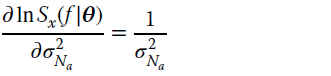
The asymptotic equation for the conditional pdf (14.7) is the basis for the CRB as the FIM entry is
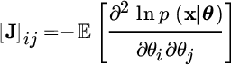
from the derivatives

Since the periodogram is asymptotically unbiased
the first term of the FIM is zero (for ![]() ) and the FIM reduces to the celebrated Whittle formula for the CRB [56] :
) and the FIM reduces to the celebrated Whittle formula for the CRB [56] :

that is generally applicable for the CRB in a broad set of spectral analysis methods.
14.3 AR Spectral Analysis
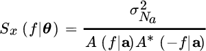
AR spectral analysis models the PSD Sx(ω) by a generation model with poles as in Figure 14.9, so that the PSD is assumed to be

for a certain order Na and excitation power ![]() . The positions of the poles in the z‐plane define the frequency and strength of the resonances, and AR is the appropriate description when the PSD shows resonances only, either because the generation mechanism is known or just assumed.
. The positions of the poles in the z‐plane define the frequency and strength of the resonances, and AR is the appropriate description when the PSD shows resonances only, either because the generation mechanism is known or just assumed.
14.3.1 MLE and CRB
In Na th order AR spectral analysis, in short AR(Na), the unknown terms are the recursive term of the filter ![]() and the excitation power
and the excitation power ![]() that depends on the specific AR order Na highlighted in the subscript:
that depends on the specific AR order Na highlighted in the subscript:
The log‐likelihood (14.7) is (apart from a scaling)
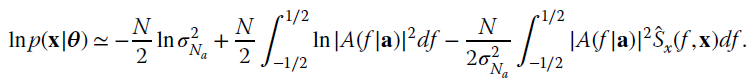
Figure 14.9 Model for AR spectral analysis.
Since for monic polynomials, ![]() (Appendix C), the log‐likelihood simplifies to
(Appendix C), the log‐likelihood simplifies to
The MLE follows by nulling the gradients in order, starting from the gradient wrt ![]() :
:

The ML estimate of the excitation power depends on the set of parameters a. Plugging into the log‐likelihood
its maximization is equivalent to minimizing ![]() wrt a. From the gradients it is (to simplify
wrt a. From the gradients it is (to simplify ![]() ):
):

Recalling that
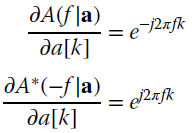
the following condition holds:
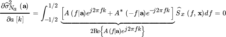
Since Ŝx(f, x) is real‐valued, ![]() , it is sufficient to solve for
, it is sufficient to solve for
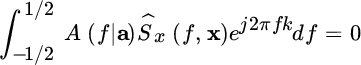
Substituting:

but recalling that the periodogram is the Fourier transform of the sample (biased) estimate of the autocorrelation, the ML estimate follows from a set of Na equations

These are the Yule–Walker equations in Section 12.3.1, here rewritten wrt the sample autocorrelation that recalls the LS approach to linear prediction (Section 12.4). Furthermore

which is the power of the excitation from the sample autocorrelation as the power of the prediction error from the Yule–Walker equations (12.4) in Section 12.3.1.
Remark: The coincidence of AR spectral analysis with the Yule–Walker equations of linear prediction is not surprising. AR spectral analysis can be interpreted as a search for the linear predictor that fully uncorrelates the process under analysis. The sample autcorrelation replaces the ensemble autocorrelation as this estimates the correlation properties from a limited set of observations with positive definite Fourier transform (while still being biased).
The CRB can be evaluated from the Whittle formula (14.8) adapted for the AR model:
Computing first the terms

and then the elements of the FIM from the Whittle formula, recalling that ![]() is causal and minimum phase4
is causal and minimum phase4
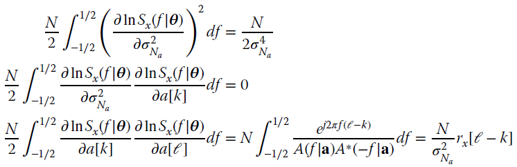
The FIM is block‐partitioned

so the estimation of the excitation ![]() is decoupled from the coefficients a of the AR model polynomial. The CRB follows from the inversion of the FIM with covariance
is decoupled from the coefficients a of the AR model polynomial. The CRB follows from the inversion of the FIM with covariance
The CRB of the coefficients a depends on the inverse of the covariance matrix Cxx. Note that all coefficients do not have the same variance, but they are unbalanced and they depend on the specific problem as discussed in the example in the next section.
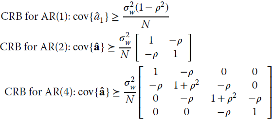
14.3.2 A Good Reason to Avoid Over‐Parametrization in AR
AR spectral analysis can be carried out regardless of the true model, or even when the PSD does not show resonances due to the presence of poles. Since the generation mechanism is not always known, the order Na of the AR spectral analysis is often another unknown of the problem at hand. Even if in principle the estimates â could account for the order as those terms larger that the true order should be zero, the augmentation of the model order in AR spectral analysis has to be avoided as the parameters a are not at all decoupled, and the covariance cov{â} could be unacceptably large.
A simple example can help to gain insight into the concept of model over‐parameterization (set an AR order in spectral analysis larger than the true AR order). Let a set of observations be generated as an AR(1) with parameters ![]() for
for ![]() (the complex‐valued case will be considered later), the autocorrelation is
(the complex‐valued case will be considered later), the autocorrelation is

and the Yule–Walker equations to estimate the parameters a leads to the estimates â such that ![]() and
and ![]() for
for ![]() (the bias
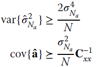
(the bias ![]() is due to the sample autocorrelation that vanishes for N large). The CRB depends on the correlation matrix Cxx that for an arbitrary order Na is structured as
is due to the sample autocorrelation that vanishes for N large). The CRB depends on the correlation matrix Cxx that for an arbitrary order Na is structured as

and its inverse is known (Section 4.5). The CRB for different order selection is:
thus showing that diagonal terms are not the same and that (for this specific problem) the CRB matrix is diagonal banded. Furthermore:

that is, the over‐parameterization increases the variance of the AR spectral analysis and the additional poles due to âk because the choice ![]() perturbs the PSD estimates that in turn depend on the dispersion of the poles.
perturbs the PSD estimates that in turn depend on the dispersion of the poles.
The conclusion on over‐parameterization is general: using more parameters than necessary reduces the accuracy of the PSD estimate so that sometimes it is better to under‐parameterize AR spectral analysis. Alternatively, one can start cautiously with low order and increase the order in the hunt for a better trade‐off, being aware that every augmentation step increases the variance of the PSD estimate.
14.3.3 Cramér–Rao Bound of Poles in AR Spectral Analysis
An AR model can be rewritten wrt the roots of the polynomial A(z) as
where μ collects all the roots ![]() as detailed below. The z‐transform of the PSD becomes
as detailed below. The z‐transform of the PSD becomes
and the Whittle relationship for the CRB of an AR spectral analysis can be rewritten in terms of the roots of the z‐transform. The importance of this model stems from the use of AR spectral analysis to estimate the angular position of the poles, and these in turn are related to the frequency of the resonances in PSD.
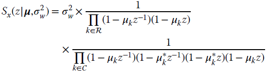
To simplify the reasoning, let the process x be real‐valued so that poles are complex conjugates μk and ![]() ; in addition poles are either real or complex but are assumed to have multiplicity one. Let the poles be decoupled into those that are real (ℛ) and those that are complex conjugates (
; in addition poles are either real or complex but are assumed to have multiplicity one. Let the poles be decoupled into those that are real (ℛ) and those that are complex conjugates (![]() ) so that the z‐transform of the PSD is
) so that the z‐transform of the PSD is
The Whittle formula needs the derivatives evaluated separately for the two sets

Integrating over the set for the elements of the FIM:5

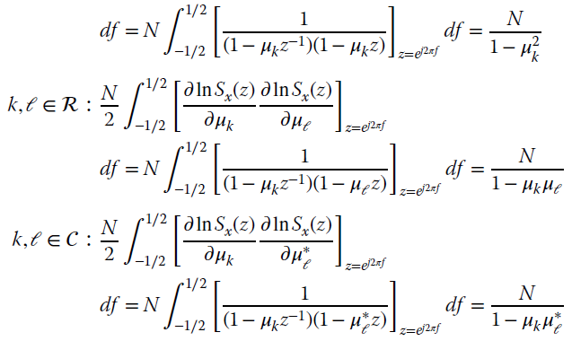
and using the identity  (Appendix C). The entries of the FIM partitioned either into real (ℛ) or complex conjugate (
![]() ) poles have the same value for the accounted pole. To summarize, it is convenient to order the Na poles into real (μℛ) and complex (
) poles have the same value for the accounted pole. To summarize, it is convenient to order the Na poles into real (μℛ) and complex (![]() ) with their conjugate (
) with their conjugate (![]() )
)

such that ![]() and
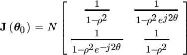
and ![]() ; so the FIM is
; so the FIM is

Example: Pole Scattering in AR(2)
Consider an AR(2) with poles ![]() . From the relationship above, the FIM is
. From the relationship above, the FIM is
To derive the covariance for real and imaginary component of the poles it is useful to recall the following identity:

so that the CRB for the transformed variables (Section 8.3) is
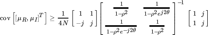
After some algebra it follows that

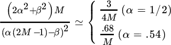
The variance of μR is independent of the frequency of the poles, and the variance for the imaginary term is very large when ![]() (both poles are coincident) and vanishes for
(both poles are coincident) and vanishes for ![]() . The error ellipsoid is not referred to the orthogonal axes, as
. The error ellipsoid is not referred to the orthogonal axes, as ![]() ; the following numerical example for AR(1) can clarify.
; the following numerical example for AR(1) can clarify.
14.3.4 Example: Frequency Estimation by AR Spectral Analysis
Let a sequence be modeled as a complex sinusoid in white Gaussian noise with power ![]()
The angular frequency ω and the amplitude ![]() are not known and should be estimated as poles in AR(1) spectral analysis. The phase of the sinusoid is denoted as
are not known and should be estimated as poles in AR(1) spectral analysis. The phase of the sinusoid is denoted as ![]() and
and ![]()
![]() . AR(1) spectral analysis models observations as
. AR(1) spectral analysis models observations as

such that ![]() and
and ![]() as the pole should approximate at best the true PSD:
as the pole should approximate at best the true PSD: ![]() . AR(1) follows from the Yule–Walker equation (12.2)
. AR(1) follows from the Yule–Walker equation (12.2)
For the sample estimate of the autocorrelation:

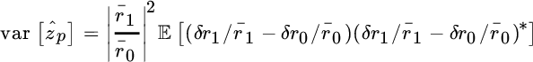
where ![]() just to ease the notation for the computations below. The objective is to evaluate the performance (bias and variance) of AR(1) spectral analysis to estimate the frequency of the sinusoid as an alternative to the conventional MLE in Section 9.3. The frequency estimate accuracy depends on the small deviations of the radial and angular position of the pole ẑp due to noise.
just to ease the notation for the computations below. The objective is to evaluate the performance (bias and variance) of AR(1) spectral analysis to estimate the frequency of the sinusoid as an alternative to the conventional MLE in Section 9.3. The frequency estimate accuracy depends on the small deviations of the radial and angular position of the pole ẑp due to noise.
Since the pole depends on the sample autocorrelations, ![]() is decomposed into (Appendix A)
is decomposed into (Appendix A)
and

For large N and large SNR defined as
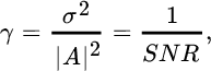
the pole can be approximated as

The bias is
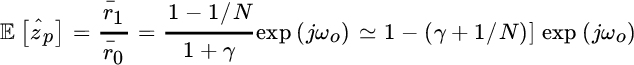
This proves that the estimate of the frequency is unbiased, but the radial position of the pole ![]() depends on γ —however for
depends on γ —however for ![]() and
and ![]() the pole attains the unitary circle. The variance is evaluated from the deviations δrk:
the pole attains the unitary circle. The variance is evaluated from the deviations δrk:
Since ![]() it is convenient to group the terms as follows
it is convenient to group the terms as follows
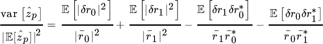
From the properties in Appendix D, the variance is

where the last approximation is for ![]() . For
. For ![]() , Figure 14.10 shows the comparison between the simulated (black solid line) and the analytical (gray dashed line) bias (14.9) (upper figure) and standard deviation
, Figure 14.10 shows the comparison between the simulated (black solid line) and the analytical (gray dashed line) bias (14.9) (upper figure) and standard deviation ![]() from (14.10) that perfectly superimpose for AR(1) and therefore validate the approximations in the sensitivity analysis for
from (14.10) that perfectly superimpose for AR(1) and therefore validate the approximations in the sensitivity analysis for ![]() and 50 samples. Figure 14.10 also shows the dispersion for AR(2) (dash dot line) when extracting only one pole corresponding to the frequency close to
and 50 samples. Figure 14.10 also shows the dispersion for AR(2) (dash dot line) when extracting only one pole corresponding to the frequency close to ![]() , that is less dispersed and closer to the unit circle for
, that is less dispersed and closer to the unit circle for ![]() .
.

Figure 14.10 Radial position of pole (upper figure) and dispersion (lower figure) for AR(1) (solid line) and AR(2) (dash dot), compared to analytic model (14.10–14.11) (dashed gray line)
In practice, the number of sinusoids is not known and it is quite common practice to “search” for the order by trial‐and‐error on the poles. Figure 14.11 shows the poles from a set of independent AR spectral analyses with order ![]() (superposition of 50 independent trails with
(superposition of 50 independent trails with ![]() and
and ![]() ) and
) and ![]() . Notice that for AR(1), the poles in every trial superimpose around the true angular position with a radial location set by the bias (14.9). When increasing the order of the AR spectral analysis, the poles cluster around the angular position in
. Notice that for AR(1), the poles in every trial superimpose around the true angular position with a radial location set by the bias (14.9). When increasing the order of the AR spectral analysis, the poles cluster around the angular position in ![]() thus providing an estimate of the frequency, while the other poles disperse within the unit circle far from the sinusoid thus allowing clear identification of the frequency of the sinusoid. However, each additional pole can be a candidate to model (and estimate) a second, or third, or forth sinusoid in observation thus providing a tool to better identify the number of sinusoids in the data (if unknown). Needless to say, ranking the poles with decreasing radial distance from the unit circle offers a powerful tool to identify the number of sinusoids, if necessary, when the number is not clear from the practical problem at hand.
thus providing an estimate of the frequency, while the other poles disperse within the unit circle far from the sinusoid thus allowing clear identification of the frequency of the sinusoid. However, each additional pole can be a candidate to model (and estimate) a second, or third, or forth sinusoid in observation thus providing a tool to better identify the number of sinusoids in the data (if unknown). Needless to say, ranking the poles with decreasing radial distance from the unit circle offers a powerful tool to identify the number of sinusoids, if necessary, when the number is not clear from the practical problem at hand.
![Model for MA spectral analysis, depicted by a rectangle labeled B(ʐ|b) with a rightward arrow at the left labeled w[n] atop and σ2MA(N b) below, and another rightward arrow at the right labeled x[n].](http://images-20200215.ebookreading.net/9/3/3/9781119293972/9781119293972__statistical-signal-processing__9781119293972__images__c14f011.gif)
Figure 14.11 Scatter‐plot of poles of Montecarlo simulations for AR(1), AR(2), AR(3), AR(4) spectral analysis.
14.4 MA Spectral Analysis
The PSD of the Nb th order moving average (MA) process is the one generated by filtering a white Gaussian noise with power ![]() with a limited support filter (or averaging filter):
with a limited support filter (or averaging filter):
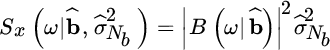
as illustrated in Figure 14.11. The MA spectral analysis estimates the set of generation parameters ![]() from the limited observations so that the PSD of the MA(Nb) model is
from the limited observations so that the PSD of the MA(Nb) model is
![Model for ARMA spectral analysis, depicted by a rectangle labeled B(ʐ|b)/ A(ʐ|a) with a rightward arrow at the left labeled w[n] atop and σ2ARMA below and another a rightward arrow at the right labeled x[n].](http://images-20200215.ebookreading.net/9/3/3/9781119293972/9781119293972__statistical-signal-processing__9781119293972__images__c14f012.gif)
From the sample estimate of the autocorrelation ![]() over the support of
over the support of ![]() samples, it is sufficient to use the identity over the z‐transform
samples, it is sufficient to use the identity over the z‐transform
and solve wrt b and ![]() , the latter acts as a scale factor of the estimated PSD. The overall problem cast in this way is strongly non‐linear and does not have a unique solution for
, the latter acts as a scale factor of the estimated PSD. The overall problem cast in this way is strongly non‐linear and does not have a unique solution for ![]() . From the sample estimate of the autocorrelation
. From the sample estimate of the autocorrelation ![]() one can extract the 2Nb roots, which are in all reciprocal positions according to the Paley–Wiener theorem (Section 4.4). These roots can be paired in any arbitrary way and collected into a set
one can extract the 2Nb roots, which are in all reciprocal positions according to the Paley–Wiener theorem (Section 4.4). These roots can be paired in any arbitrary way and collected into a set ![]() provided that each selection does not contain the reciprocal set. Even if any collection of zeros in the filter
provided that each selection does not contain the reciprocal set. Even if any collection of zeros in the filter ![]() is an MA estimate, the preferred one is the minimum phase arrangement
is an MA estimate, the preferred one is the minimum phase arrangement ![]() so that
so that
This is essential for the MA analysis of the sample autocorrelation, and some remarks are necessary to highlight some practical implications.
Remark 1: To reduce the variance of the sample estimate of the autocorrelation, it is customary to average the sample estimate after segmenting the set of observations into M subsets of disjoint time series of ![]() samples each. Assuming
samples each. Assuming ![]() to be the mth segment, the sample autocorrelation is
to be the mth segment, the sample autocorrelation is
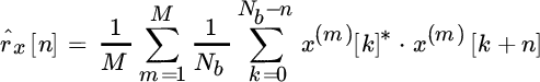
and the variance for disjoint sets decreases with 1/M. Of course, the order of the MA analysis should be traded with the variance of the sample autocorrelation.
Remark 2: Given the sample autocorrelation over an arbitrary interval, say ![]() , MA(Nb) cannot be carried out by simply using the first Nb samples (that would imply a truncation of the sample autocorrelation) but must rather be by windowing the autocorrelation by a window
, MA(Nb) cannot be carried out by simply using the first Nb samples (that would imply a truncation of the sample autocorrelation) but must rather be by windowing the autocorrelation by a window ![]() that has a positive definite FT (
that has a positive definite FT (![]() for
for ![]() but
but ![]() for any ω). To justify this, let
for any ω). To justify this, let
be the sample autocorrelation over N samples; the FT ![]() has the following property (Appendix A):
has the following property (Appendix A):
To carry out MA(Nb) spectral analysis, the sample autocorrelation ![]() is windowed and the MA spectral analysis becomes
is windowed and the MA spectral analysis becomes
for some choice of ![]() . The MA PSD is biased, as
. The MA PSD is biased, as

and it is biased for ![]() as
as ![]() . The choice of the window should guarantee that
. The choice of the window should guarantee that ![]() to make the PSD positive definite. Truncation
to make the PSD positive definite. Truncation ![]() for
for ![]() would not satisfy this constraint, while
would not satisfy this constraint, while ![]() for
for ![]() (triangular window) fulfills the constraints and is the most common choice.
(triangular window) fulfills the constraints and is the most common choice.
14.5 ARMA Spectral Analysis
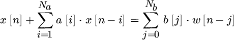
ARMA(Na, Nb) spectral analysis is the composition of the AR(Na) and MA(Nb) systems. Namely, the ARMA process is obtained from the causal linear system excited by white Gaussian process w[n] as described by the difference equation (Figure 14.13)
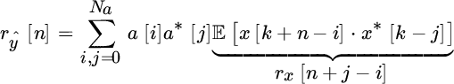
The constitutive relationship of ARMA can be derived from the definition of the autocorrelation
using the second form of the finite difference equation (14.11) by multiplying for ![]() and computing the expectation:
and computing the expectation:
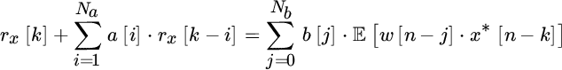
Figure 14.13 Model for ARMA spectral analysis.
Since the system is causal, the impulse response is h[n] and the process x[n] is the filtered excitation:

Substituting into the second term of the relationship above:

and thus

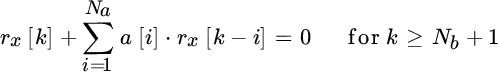
In this form it is still dependent on the impulse response, but since ![]() for
for ![]() (causal system), the second term is zero for
(causal system), the second term is zero for ![]() and also for
and also for ![]() . It follows the modified Yule–Walker equations:
. It follows the modified Yule–Walker equations:
which is a generalization of the Yule–Walker equations for the ARMA processes to derive the AR(Na) component â of the ARMA(Na, Nb). Of course, for ARMA analysis from a limited set of samples x[n], the autocorrelation is replaced by the sample (and biased) estimate of the autocorrelation (Appendix A).
After solving for the modified Yule–Walker equations (14.12) to get â, one solves for MA(Nb). This is obtained by noticing that when filtering the observations with ![]() (incidentally, this is the prediction error using a linear predictor based on the modified Yule–Walker equations) obtained so far, the residual depends on the MA component only as
(incidentally, this is the prediction error using a linear predictor based on the modified Yule–Walker equations) obtained so far, the residual depends on the MA component only as
The autocorrelation of the MA component ![]() :
:
rewritten in the form of sample autocorrelation (recall that ![]() )
)

Therefore, the ![]() samples of the autocorrelation
samples of the autocorrelation ![]() represent the MA component of the ARMA process and can be estimated following the same rules as MA(Nb) applied now on
represent the MA component of the ARMA process and can be estimated following the same rules as MA(Nb) applied now on ![]() . By using the identity
. By using the identity
it can be solved for b and the excitation power ![]() that is now the scaling factor for the whole ARMA process.
that is now the scaling factor for the whole ARMA process.
Remark 1: Note that there is no guarantee that the sample autocorrelation ![]() holds over the range
holds over the range ![]() , so the PSD of the MA component may not be positive semidefinite. In this case it is a good rule when handling sample estimates (that could have some non‐zero samples outside of the range of the MA process) to window
, so the PSD of the MA component may not be positive semidefinite. In this case it is a good rule when handling sample estimates (that could have some non‐zero samples outside of the range of the MA process) to window ![]() with a triangular window over the range of the order of the MA component, as this guarantees that the PSD is positive definite.
with a triangular window over the range of the order of the MA component, as this guarantees that the PSD is positive definite.
Remark 2: The estimate of the AR portion by the modified Yule–Walker equation (14.12) with the sample autocorrelation could be slow, as the system of equations uses samples with lower confidence (as for ![]() ). Some alternative methods could be explored to make a better (and more efficient) use of the available samples.
). Some alternative methods could be explored to make a better (and more efficient) use of the available samples.
14.5.1 Cramér–Rao Bound for ARMA Spectral Analysis
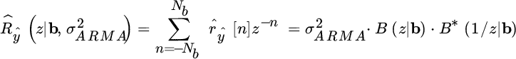
Let the PSD for the ARMA be

where ![]() and
and ![]() are both minimum phase factorizations (a and b are real‐valued vectors). The CRB is obtained from the asymptotic Whittle formula starting from:
are both minimum phase factorizations (a and b are real‐valued vectors). The CRB is obtained from the asymptotic Whittle formula starting from:
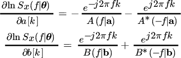
The second order derivatives for the FIM elements are (recall the causality condition for the factorizations ![]() and
and ![]() ):
):
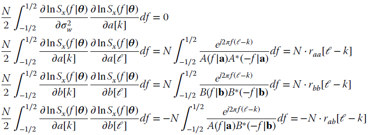
where raa[k], rbb[k], rab[k] are the auto/cross‐correlation sequences for two equivalent AR processes and a mixed one, all excited by a unit‐power white process:
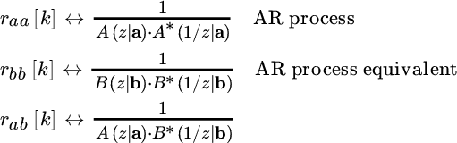
Autocorrelation raa[k] and rbb[k] of the AR processes can be numerically evaluated from the Yule–Walker equations for the polynomials ![]() and
and ![]() , respectively. The numerical computation of the cross‐correlation rab[k] deserves a comment as the following factorization of
, respectively. The numerical computation of the cross‐correlation rab[k] deserves a comment as the following factorization of

highlights the way to compute it. Namely, first the Yule–Walker equations are applied to compute the autocorrelation for the equivalent AR process ![]() represented by the first term using the minimum phase factorization
represented by the first term using the minimum phase factorization ![]() , and then the cross‐correlation terms of interests are obtained by filtering the autocorrelation computed thus far with a finite impulse non‐causal (as
, and then the cross‐correlation terms of interests are obtained by filtering the autocorrelation computed thus far with a finite impulse non‐causal (as ![]() is non‐causal) filter
is non‐causal) filter ![]() .
.
The FIM is block‐partitioned:

with blocks

The structure of the FIM confirms that for ARMA spectral analysis the AR and MA parameters are coupled, and this offers room to find different estimation procedures than in Sections 14.3–14.4, but the power of the excitation acting as a scale parameter is always decoupled. This decoupling is not surprising as the structure of the PSD in terms of resonances and nulls depends on the poles and zeros of the AR and MA components, but not on the scale factor. The CRB for ARMA spectral analysis can be considered the more general one as the CRB for AR and MA can be derived from the CRB of ARMA by removing the corresponding blocks.
Appendix A: Which Sample Estimate of the Autocorrelation to Use?
Given N samples of a random process ![]() , the sample estimate of the autocorrelation is:
, the sample estimate of the autocorrelation is:
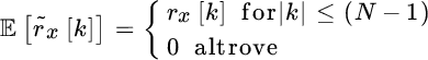
However, this sample estimate is biased as for every value of the shift k the product terms that are summed up are ![]() ; analytically it is
; analytically it is

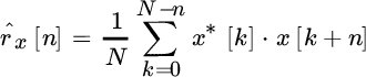
Alternatively, one can avoid the bias by scaling the sum for the number of terms, and it follows the definition of the sample autocorrelation
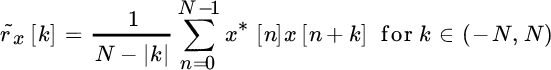
which is unbiased as
Herein we prove that even if the estimate ![]() is apparently the preferred choice being unbiased, the biased estimate of the sample autocorrelation
is apparently the preferred choice being unbiased, the biased estimate of the sample autocorrelation ![]() is the choice to be adopted in all spectral analysis methods.
is the choice to be adopted in all spectral analysis methods.
The Fourier transform of the two sample estimates are
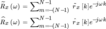
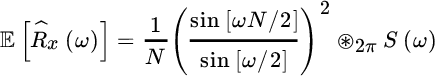
The expectations are related to the PSD Sx(ω) as follows
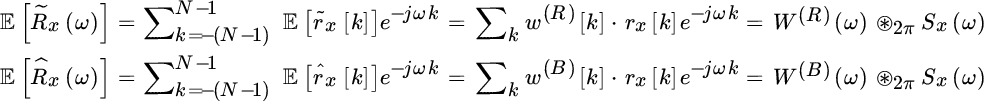
where the limited support autocorrelation has been replaced by rectangular and triangular (or Bartlett) windowing
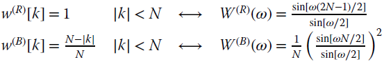
Inspection of the relationships (14.13) proves that the FT of the unbiased sample autocorrelation ![]() is not positive definite as W(R)(ω) could be negative valued, for some spectral behaviors. On the other hand, the Fourier transform of the biased sample autocorrelation
is not positive definite as W(R)(ω) could be negative valued, for some spectral behaviors. On the other hand, the Fourier transform of the biased sample autocorrelation ![]() is positive definite (in the mean) as the sample estimate is implicitly windowed by a Bartlett window w(B)[k] that has positive definite FT. Furthermore, it can be seen that for
is positive definite (in the mean) as the sample estimate is implicitly windowed by a Bartlett window w(B)[k] that has positive definite FT. Furthermore, it can be seen that for ![]() , the Bartlett windowing becomes a constant and
, the Bartlett windowing becomes a constant and ![]() , therefore
, therefore
is the unbiased estimate of the PSD. Incidentally, the biased sample autocorrelation is the implicit estimator used by the periodogram in PSD estimation.
Appendix B: Eigenvectors and Eigenvalues of Correlation Matrix
The objective here is to show the equivalence between the eigenvectors of a correlation matrix with Toeplitz structure and the basis of the discrete Fourier transform (DFT). A few preliminary remarks are in order. Given a periodic sequence {e[n]} with period of N samples, the circular (or periodic) convolution over the period N with a filter {h[n]} is equivalent to the linear convolution ![]() made periodic with period N
made periodic with period N

The DFT of the circular convolution is
where
is the DFT of the sequence ![]() (recall that
(recall that ![]() is the Nth root of unitary value). In compact notation, the DFT is
is the Nth root of unitary value). In compact notation, the DFT is
where WN is the matrix of forward DFT (it has a Vandermonde structure). Since the inverse DFT is
it follows that
Here, the columns of WN are a complete basis ℂN and each column represents a complex exponential exp(j2πnk/N) of the DFT transformation. The circular convolution after DFT is
where
The properties of an arbitrary covariance matrix Cxx are derived by assuming that random process x is the output of a linear system with Gaussian white input
so that the following property holds for its DFT:
Since ![]() , the covariance matrix is
, the covariance matrix is
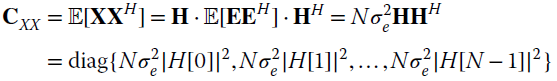
but still from the definitions of covariance matrix and DFT:

leading to the following equality:
Each column of the DFT basis is one eigenvector of the covariance matrix Cxx obtained after circular convolution, and the entry ![]() is the corresponding eigenvalue. Resuming the definition of eigenvectors/eigenvalues with an orthonormal basis:
is the corresponding eigenvalue. Resuming the definition of eigenvectors/eigenvalues with an orthonormal basis:
where the k th eigenvector and eigenvalue are
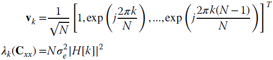
notice that the k th eigenvalue coincides with the power spectral density
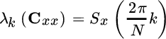
Based on these numerical equalities, some remarks are now necessary to better focus on the importance of the results derived so far.
Remark 1: For a stationary random process, the eigenvector decomposition of the covariance matrix Cyy is
In general, the kth eigenvector ![]() , and similarly
, and similarly ![]() as the process x[n] is not periodic, or it was not generated as circular convolution over a period N. However, for a very large period N, the periodic and linear convolution coincides, except for edge effects that become negligible for large N. The same conclusion holds for the covariance if
as the process x[n] is not periodic, or it was not generated as circular convolution over a period N. However, for a very large period N, the periodic and linear convolution coincides, except for edge effects that become negligible for large N. The same conclusion holds for the covariance if ![]() (in practice, it is enough that N is larger than the coherence interval of the process x[n], or equivalently the covariance matrix Cxx is a diagonal banded matrix with a band small enough compared to the size of the covariance matrix itself):
(in practice, it is enough that N is larger than the coherence interval of the process x[n], or equivalently the covariance matrix Cxx is a diagonal banded matrix with a band small enough compared to the size of the covariance matrix itself):
Remark 2: In software programs for numerical analysis, the eigenvectors of the covariance matrix are ordered for increasing (or decreasing) eigenvalues while power spectral density ![]() is ordered wrt increasing frequency as the eigenvectors are predefined as the basis of the Fourier transform.
is ordered wrt increasing frequency as the eigenvectors are predefined as the basis of the Fourier transform.
Remark 3: In the case of a complex‐valued process, it is convenient to partition the DFT into real and imaginary components:
where each of the vectors are (Section 5.4)

and the following properties of orthogonality hold:

In summary

and thus
as expected.
Appendix C: Property of Monic Polynomial
This Appendix extends some properties of the z‐transform in Appendix B of Chapter 4. Let H(z) be the monic polynomial of a minimum phase filter ![]() excited by a white Gaussian noise with unitary power (
excited by a white Gaussian noise with unitary power (![]() ); the z‐transform of the autocorrelation sequence is
); the z‐transform of the autocorrelation sequence is
Since along the unitary circle the Fourier transforms ![]() and
and ![]() are positive semidefinite, after the log as monotonic transformation:
are positive semidefinite, after the log as monotonic transformation:
The careful inspection of
proves that since H(z) is minimum phase, it is analytic for ![]() (poles/zeros are for
(poles/zeros are for ![]() ), and from the properties of the log it follows that poles/zeros are transformed as follows: zeros of
), and from the properties of the log it follows that poles/zeros are transformed as follows: zeros of ![]() poles of ln H(z); poles of
poles of ln H(z); poles of ![]() poles of ln H(z). Since H(z) is minimum phase, the polynomial
poles of ln H(z). Since H(z) is minimum phase, the polynomial ![]() is minimum phase also. From the initial value theorem
is minimum phase also. From the initial value theorem ![]() (monic polynomial) and thus
(monic polynomial) and thus ![]() , hence6
, hence6

and thus
Appendix D: Variance of Pole in AR(1)
The biased estimate of the autocorrelation is (sample index is by subscript):

and the mean value is

To compute the variance it is necessary to evaluate the expectation for all mixed terms ![]() . After some algebra:
. After some algebra:

and the expectations are
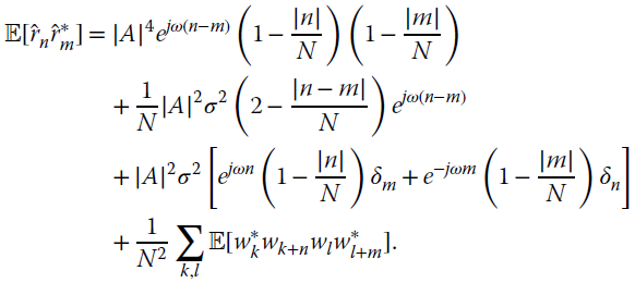
Under the assumption that ![]() and
and ![]() , one can specify the following moments:
, one can specify the following moments:
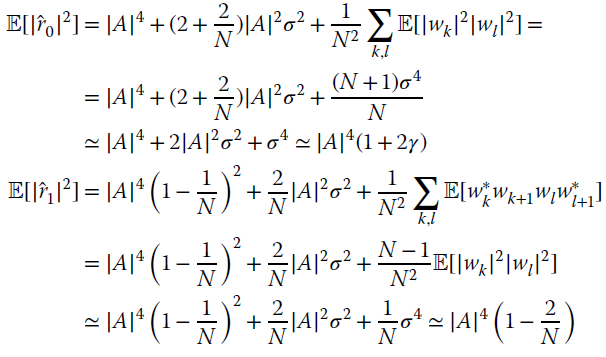
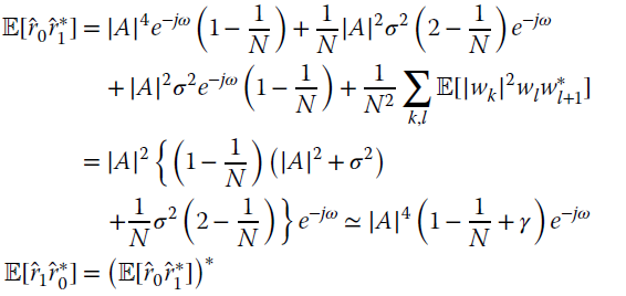
Recalling that the random term in the sample estimate is redefined as deviation wrt the mean value ![]() , it follows that:
, it follows that:
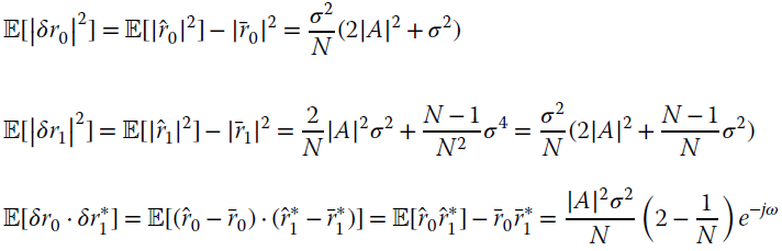
these are useful for the derivation in the main text.