
4
SAR Interferometry: Principles and Processing
Philippe DURAND1, Nadine POURTHIÉ1, Céline TISON1 and Giorgio GOMBA2
1CNES, Toulouse, France
2German Aerospace Center (DLR), Oberpfaffenhofen, Germany
4.1. Introduction
Synthetic aperture radar interferometry (InSAR) combines two SAR single-look-complex (SLC) images to exploit the geometrical information contained in the phase difference. The phase of the electromagnetic wave describes, among other contributions, the wave propagation path. This access to the geometry is very valuable for describing the topography of the illuminated terrain. By combining more than two phases, InSAR allows the measurement of the topography changes by minimizing the phase noise.
To obtain accurate measurements of the wave path difference, the conventional InSAR technique computes the normalized complex correlation coefficient called the coherence. The coherence argument provides the wrapped phase image (value ranging from 0 to 2π) called the interferogram. It is related to the acquisition geometry and topographic/displacement information. The coherence modulus (value ranging from 0 to 1) provides for each pixel an indicator of the similarity of the two SAR complex images. It is related to the phase noise and characterizes the geometric phase reliability, as explained later in this chapter.
The inversion of the interferometric phase delivers direct information on the surface topography, provided that the satellite orbit and a reference geoid are accurately defined. Furthermore, the measurement of the variations of topography gives a surface displacement map, leading to the concept of differential interferometry. Differential interferometry (DInSAR) is the combination of two interferograms or one interferogram and a reference digital elevation model (DEM)1. The DInSAR method enables movement detection at a fraction of the radar wavelengths (i.e. a few millimeters).
In this chapter, interferometry principles are explained. The limits of the method are also discussed (coherence loss, relief impact in shadows and layovers, atmospheric artifacts, etc.). A particular emphasis is put on the atmospheric impacts, which are a major issue for displacement observations. In fact, displacement detection requires the combination of interferograms acquired at different times, sometimes with quite a large gap. The meteorological conditions are thus often different. The water content of the atmosphere disturbs the radar phase, which can mislead the DInSAR interpretation. The interferometric processing steps are illustrated on the basis of Differential Interferometric Automated Process in the ORFEO Tool Box (DiapOTB) processors. This open source interferometric toolbox, made available by CNES in the framework of the Orfeo ToolBox (OTB), is one of the available interferometric software packages. The main processing steps are common to all the approaches, with a key point being the registration. Intrinsic decorrelation due to the native geometry and surface changes can affect the quality of the interferogram, and the remaining quality improvement comes from the registration accuracy of both images.
4.2. Principle and limits of SAR interferometry
The phase of SLC images depends on the geometric path of the electromagnetic waves. Interactions with the backscattering surface or volume (forest, snow/ice, etc.) can also modify it so that the phase of each pixel is tainted by speckle noise due to the physical properties and spatial distribution of the elementary targets within the corresponding resolution cell.
The main idea of interferometry is to combine two SAR images acquired with very similar geometries. To measure the topography, a baseline (i.e. a geometrical difference between the two sensor positions) is necessary to create slightly different viewing angles in the acquisitions, as in an optical stereo configuration. Note that the magnitude of the B/H ratio is much lower in SAR imagery than in optical imagery. The accuracy of the estimated topography benefits from a large baseline. The limits for the baseline/height (B/H) ratio for InSAR were introduced in Chapter 1, section 1.1.2. However, this geometrical difference has to be small enough to limit the speckle noise decorrelation, leading to an important trade-off between noise level and geometric accuracy. Indeed, speckle is a deterministic phenomenon: its realization will be similar in both images if the surface has not changed and the geometries of the images are close enough. For the measurement of displacement by differential interferometry using an available DEM, this geometric difference should be as small as possible: the differential interferogram will be less affected by DEM errors and the phase noise from different speckle realizations.
4.2.1. Geometrical information
Most interferograms are computed from two SAR images acquired by the same sensor with two different positions in space and time. In some cases, interferometry is performed with two antennas, with one emitting and both receiving simultaneously, either on the same platform, as in the Shuttle Radar Topographic Mission (SRTM), or on two platforms flying on simultaneous parallel orbits, such as the TerraSAR-X/TanDEM-X satellites. This configuration is referred to as the bistatic case.
In the following, we only consider the monostatic case: acquisition of two separate images by the same sensor at two different dates (also called repeat-pass interferometry). The bistatic case involves the same geometric behavior as the monostatic one, except that the travel path difference is divided by two since only the return path is different. The bistatic case has the advantage of not being affected by atmospheric disturbances and ground surface changes in the quasi-simultaneous bistatic acquisitions. All the other processing issues are the same.
Figure 4.1 provides the InSAR geometry and the notations used in the following text. The geometric distance between the two positions of the sensor, called the “baseline”, B, is a fundamental parameter. Its importance for the signal quality is discussed in section 4.2.2. In this section, we first provide the major equations for the understanding of interferometry. B⊥ is the orthogonal baseline after projection onto the direction perpendicular to the range vector. B⊥ and the incidence angle θ are the main factors in the InSAR geometric equations.
The interferometric phase is linked to the differential geometric path of the electromagnetic wave:
where λ is the wavelength and R2 and R1 the range distance between one point and the two satellite positions. The differential geometric path φ can be decomposed into several contributions:
with φorb being the orbital phase (flat terrain phase referenced on a geoid), φtopo the topographic phase, φdis the phase due to surface displacement, φaps the differential atmospheric phase screen (APS) and φnoise the differential phase noise.
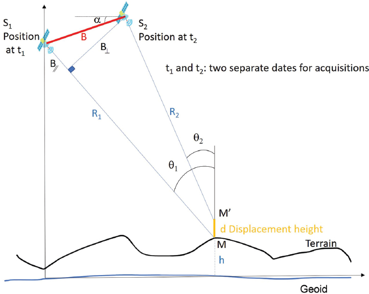
Figure 4.1. Interferometry geometry and the notation used in this chapter. For a color version of this figure, see www.iste.co.uk/cavalie/images.zip
The expressions of φorb, φtopo and φdis are as follows (Rosen et al. 2000), with B⊥ being the orthogonal baseline and θ the incidence angle:


where dLOS is the projection of the displacement on the radar line-of-sight (LOS); for a vertical displacement d illustrated in Figure 4.1, dLOS = d cos θ.
φorb is estimated and removed by considering the terrestrial geoid surface and the orbit directly in the registration process. For surface displacement applications, φtopo is removed by considering a reference DEM or by using a second interferogram. The quality of the orbit, the geoid and the DEM are essential for the final accuracy of the estimation. For displacement analysis, the focus is placed on φdis. For TOPSAR and spotlight modes, a specific phase correction is needed to avoid the misalignment variations (the squint angle varies during the acquisition). This correction, commonly called deramping or reramping, should be performed before the coregistration of the two images.
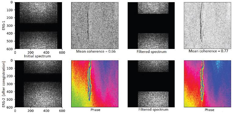
Figure 4.2. Illustration of frequency shift in the interferometric pair. The spectra are filtered to retain the common part and enhance the coherence at the price of a loss in resolution. ERS-1/ERS-2 interferogram (May 2 and 3, 1995, Isla Incahuasi in the center of the Salar de Uyuni, Bolivia). For a color version of this figure, see www.iste.co.uk/cavalie/images.zip
The registration also induces a slight frequency shift between the two images, leading to a decorrelation term ρgeo. This is due to the ground projection of the frequency (Fornaro and Guarnieri 2002). Figure 4.2 shows that retaining only the common part of the two image spectra after the coregistration (common band filtering) can increase the InSAR coherence. For ERS satellites, the frequency shift was very important and could not be ignored. With the new SAR system, this shift is minimized. The InSAR processor may even skip this correction to preserve the spatial resolution, which is the case for DiapOTB. The impact of the decorrelation is acceptable in these cases.
Figure 4.3 illustrates the wrapped phase in an interferogram computed from a Sentinel-1 Stripmap pair, first when no corrections are applied, and second when topographic and orbital fringes are removed, leaving only displacements and residual tropospheric delays.
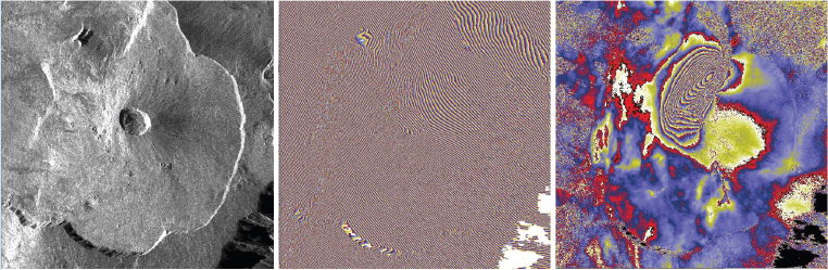
Figure 4.3. An interferogram with and without topographic and orbital fringes (Sentinel-1 Stripmap, Piton de la Fournaise area, Reunion Island). The differential interferogram very clearly highlights the ground motion due to the volcanic eruption on September 11, 2016. Left: intensity image, middle: interferogram, right: differential interferogram. For a color version of this figure, see www.iste.co.uk/cavalie/images.zip
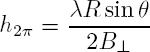
From the previous definitions, it is clear that the altitude of ambiguity h2π is the altitude difference which corresponds to a complete 2π round of the interferometric phase :
Then, knowing the phase difference δφ, the height difference δh can be deduced as:
As an example, if a 100 m perpendicular baseline is used with θ = 35°, a 2π change of the interferometric phase corresponds to an altitude difference (h2π) of about 131 m for Sentinel-1 (C-band, R = 826 km), 66 m for CSK (X-band, R = 741 km) and 54 m for TSX (X-band, R = 614 km).
Since the phase of the interferogram is measured modulo 2π, the elevation is the observed modulo h2π. Here, h2π gives the sensitivity of the DEM used. The smaller the h2π is, the better the DEM. If the DEM is old (or not accurate) and topographic changes occur before image acquisition, then fringes proportional to the changes will appear. Each fringe will represent an error of h2π in the interferogram. This will cause errors in the phase unwrapping and may be misinterpreted as a displacement. In this case, a small h2π (large baseline) is a disadvantage. h2π should be chosen as not too small with respect to the DEM variations. Phase unwrapping methods are discussed in Chapter 6.
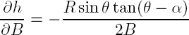
As a consequence, the uncertainty of h with respect to φ and B is equal to:

In addition, the digitization of the signal implies a quantification noise in the interferometric phase. The impact of this noise on the height accuracy depends directly on h2π.
In order to measure surface displacement, differential interferograms are computed from at least three SAR images or two SAR images and a DEM. Differential interferometry aims to remove the contribution of the DEM and obtain only the topographic variations.
4.2.2. How to choose an interferometric pair?
The baseline B between the two acquisitions should be carefully chosen. A first criterion is respect of the critical baseline. Inside the pixel resolution cell, there is a geometrical difference between the closest part of the pixel and the farthest part of the pixel. This creates a phase difference inside the pixel (Figure 4.4). If this difference is higher than λ/2 in two acquisitions, the speckle due to distributed scatterers within the resolution cell will not be correlated for the two acquisitions. In contrast to noise reduction in intensity images where the decorrelation of speckle is the key, the conventional InSAR approach seeks speckle correlation to erase the speckle phase. Note that this constraint disappears when a single dominant scatterer is present in the resolution cell, as in the permanent scatterer (PS) approach (see Chapter 5). The critical baseline is thus the maximum baseline, which guarantees a correlation of the speckle within the pixel:
At the pixel level, the interferometric condition is:
The limit of this critical baseline for InSAR processing is when the common part of the two SLC spectra becomes null.
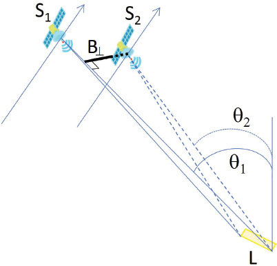
Figure 4.4. Condition between view angles to guarantee internal correlation inside the pixel.B⊥ should not be too large in order to guarantee that the internal path delay is below  For a color version of this figure, see www.iste.co.uk/cavalie/images.zip
Therefore, the baseline should not be too large in order to meet the requirement with respect to B⊥c.
For Sentinel-1, Δr = 2.33 m, R = 826 km, θ = 35° and B⊥c = 6884 m, which largely exceeds a fixed orbital tube of 100 m. The orbital tube ensures ground-track coverage repetitiveness and consequently ensures repeat-pass interferometric compatibility between SAR images acquired on the same orbit. The size of the orbital tube may also have an impact on the interferometric performance in terms of azimuth spectral decorrelation and azimuth coregistration accuracy under the presence of squint. These effects require special consideration for ScanSAR, spotlight and TOPSAR modes (Prats-Iraola et al. 2015).
When using an interferogram dedicated to DEM generation, the second constraint on the baseline is the ambiguity altitude. From equation [4.8], the smaller the h2π is, the more precise the estimation of h is. However, h2π should not be overly small compared to the local topography in order to avoid too many phase wrappings, which can result in narrow fringes or even signal aliasing when the phase rotation between adjacent pixels is higher than π. The eligible SLC pairs are thus the ones checking the two conditions on B⊥: B⊥ below the critical baseline and B⊥ leading to a suitable h2π. In other words, the common part of the spatial spectrum must be large enough.
With C-band wavelengths, baselines lengths between 30 m and 70 m are useful for surface change detection and baselines smaller than 30 m are needed to study the movements of the Earth’s surface. For the generation of an InSAR DEM, the optimal perpendicular baseline is in the range of 150–300 m. However, the best result is achieved by using a combination of interferograms with different h2π. Indeed, interferograms with small baselines can be used to help unwrap interferograms with high baselines.
4.2.3. Phase and coherence estimation
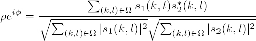
The phase difference between two coregistered SLC images s1 and s2 can be obtained at each pixel (k, l) by the Hermitian product ![]() However, to reduce the phase noise and to estimate the coherence, spatial averaging is necessary. If Ω denotes the averaging window (boxcar, adaptive, etc.), the interferogram φ and its coherence ρ are estimated as (Rosen et al. 2000):
However, to reduce the phase noise and to estimate the coherence, spatial averaging is necessary. If Ω denotes the averaging window (boxcar, adaptive, etc.), the interferogram φ and its coherence ρ are estimated as (Rosen et al. 2000):
By analogy with the processing of intensity images, this initial spatial averaging is (abusively) called complex multi-looking and the number of SLC pixels averaged is called the number of looks L. This formula implies that the L looks are fully decorrelated. This strong hypothesis is not always true, as the impulse response of the instrument and the nature of the ground may induce some spatial correlations between pixels. Nonetheless, modeling the inter-pixel correlation is not straightforward and the number of looks is often assimilated as the number of averaged pixels at native SAR resolution.
Despite this initial complex multi-looking, the phase and the coherence values estimated in equation [4.12] are still noisy. The noise level depends on the true coherence level D and the number of independent looks L. The phase statistics are ideally described by a probability distribution function (PDF) of the interferometric phases given by equation [4.13] (Tupin et al. 2014) and illustrated in Figure 4.5.

where 2F1 represents a hypergeometric function.
The noise characteristics of interferometric phases can play an important role in InSAR performance. For example, these statistics can be used for maximum likelihood estimation of different parameters of interest, such as deformation, deformation rate and topography, and can also be used for uncertainty (precision and reliability) descriptions of these products.

Figure 4.5. Phase probability density functions (PDFs) according to the level of coherenceD and the number of independent looksL

Figure 4.6. Left: coherence probability density functions (L = 6 ); right: the estimated coherence for different numbers of looks
The coherence value is between 0 and 1; the closer to 1, the more reliable the φ is. Equation [4.12] provides an estimate of the coherence value ρ, but this estimate is biased and its variance depends on the true coherence D and the number of looks L, as illustrated in Figure 4.6. The coherence PDF is given by equation [4.14] and the first- and second-order moments by equations [4.15] and [4.16], respectively (Tupin et al. 2014):
Moreover, coherence estimation implies spatial averaging of the data inside a given estimation window (equation [4.12]). This estimation technique relies on the hypothesis that all the signals involved in the estimation process are locally stationary. When this is not the case, biased coherence values result. For example, if phase values due to the topography are not properly compensated for, the estimated coherence value is underestimated.
4.2.4. Loss of coherency: several reasons
Low-coherence areas in InSAR results show low degrees of similarity between echoes into these areas, and consequently phase difference with low coherence does not completely represent the distance difference between echoes. In addition, coherence can reflect whether the terrain changes during the interval between the two illuminations, and it can also be used as an index of SAR image classification. The quality of an interferogram can be measured by estimating the coherency of the data, but this coherency is affected by many factors, such as Doppler centroid difference, the baseline and atmospheric effects. Accordingly, the coherence can be written as (Rosen et al. 2000):
with ρtemp being the temporal decorrelation due to surface changes, ρgeo the geometrical decorrelation due to the perpendicular baseline B⊥, ρvol the volumic decorrelation, ρDoppler the Doppler decorrelation due to different squints in the acquisitions, ρcor the decorrelation due to coregistration errors, ρ2π the decorrelation due to the h2π value, ρquant the decorrelation due to signal quantization and ρSNR the decorrelation due to the image SNR.
Coherency drops may be due to various phenomena, mainly atmospheric content or drastic changes in the soil (vegetation growing, a change in moisture conditions, surface modification, impact of wind on trees or bare soils), as these change the scattering element geometry or dielectric properties, reducing the interferometric correlation. Low correlation values (< 0.3) significantly reduce interferogram quality, and the measurement of topography or motion is then difficult.
The longer the time intervals are between image acquisitions, the more likely it is that the coherence will drop. For differential interferometry, the reference image has to be carefully chosen to assure the best coherence between dates. In Figure 4.7, we can clearly see a loss of coherence in a pair separated by 12 days compared with a four-month-interval case.
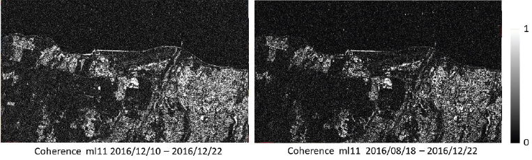
Figure 4.7. Coherence images computed with a 12 day interval (left) and a 4 month interval (right) from Sentinel-1 images of the Saint Denis area (Réunion Island). The coherence is higher with the 12 day pair, especially for natural surfaces for which it is otherwise quite low. For human-made structures, the coherence can stay high if there is no modification
In practice, low coherence values are often due to a change in the observed surface (e.g. vegetation growing, impact of wind on the surface, movements), atmospheric conditions or a very large difference in the geometry (baseline too large; see section 4.2.2). One way to optimize the coherence is to privilege a small baseline and small time spacing between the images.
4.2.5. Other InSAR limitations
One limitation of using the conventional InSAR technique is temporal and/or geometrical decorrelations in areas with large deformation rates and/or with dense vegetation.
For DEMs with steep slopes, layovers and shadows may occur. Layovers are areas where the radar backscattered signal from the ground and that from the relief are mixed (see Chapter 3, section 3.1.1). This occurs when ground and relief are at the same range distance from the sensor. For instance, in mountainous or urban areas, there are many layovers because of the high steepness of the terrain. Unmixing is a very tricky operation, and layovers are mostly considered as lost information. Shadows are due to areas inaccessible to the radar signal, mainly in mountainous regions where mountains hide the ground behind them. In such conditions, interferograms cannot provide information. As a result, ground movement monitoring in mountainous regions is always challenging. However, these are regions highly susceptible to earthquakes and thus ground motions.
Conventional SAR interferometry does not work with an InSAR monostatic configuration over water (especially smooth open water) because the surface returns little backscattered energy to the SAR antenna (specular reflection) and it is constantly changing (low coherence). There are some methods that can combine multiple interferograms and potentially increase the signal strength of river areas, so that the absolute phase information of the water level is obtained to provide spatio-temporal dynamics of the river levels. Special modes and wavelengths, such as near-nadir Ka-band InSAR, allow strong water/land radiometric contrast (typically of the order of 10 dB) and very high interferometric coherence on water. The Ka-band radar interferometer (KaRIn) of Surface Water and Ocean Topography (SWOT), the NASA/CNES wideswath altimetry mission scheduled to launch at the end of 2022 (Fjortoft et al. 2014), is a bistatic system especially designed for interferometry over oceans and in-land waters.
DEM accuracy influences the final precision of deformation monitoring, especially when processing DInSAR with only one image pair. The DEM grid resolution, the DEM height precision and the DEM’s being up-to-date with regard to the InSAR images processed should be considered. The theoretical limit is λ/4 for proper deformation monitoring. When the dataset includes a lot of images (typically more than 20 with more widely spread perpendicular baselines), the InSAR results are less impacted by DEM errors (Lazecky et al. 2015).
4.3. Atmospheric corrections
4.3.1. Compensation for tropospheric delays
Due to the presence of air in the atmosphere, electromagnetic waves travel at lower speeds than in the near-vacuum that prevails at the satellite altitude. As a result, the back-and-forth travel time of a radar pulse emitted by a SAR satellite experiences a delay, so that the total travel time cannot simply be converted into a geometric distance between the satellite and the ground target. The total excess atmospheric delay experienced by the radar wave typically amounts to an apparent one-way zenithal excess length of approximately 3 meters at sea level altitude and temperate latitudes. Unfortunately, due to the dynamic nature of the Earth’s atmosphere, this atmospheric delay varies temporally, laterally and vertically. As a result, SAR interferograms are commonly affected by atmospheric artifacts, manifesting as distortions in the fringe patterns, eventually affecting the quality of the resulting geodetic measurements (Massonnet and Feigl 1995; Zebker et al. 1997).
In the microwave range, the speed of light is mainly affected by air pressure (P ), air temperature (T ) and water vapor pressure (e). The total one-way tropospheric delay (in meters) from the satellite to a ground pixel at elevation z can be expressed as (Baby et al. 1988; Doin et al. 2009):
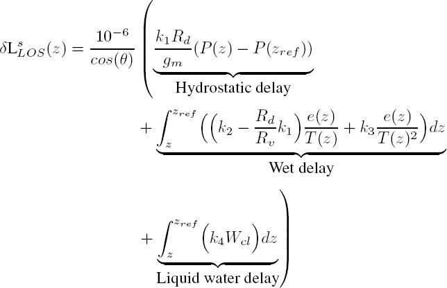
where θ is the local incidence angle, Rd = 287.05 J.kg−1.K−1 and Rv = 461.495 J.kg−1.K−1 are, respectively, the dry air and water vapor specific gas constants, gm is a weighted average of the gravity acceleration between z and zref, P is the dry air partial pressure in Pa, e is the water vapor partial pressure in Pa, T is the temperature in K and Wcl is the cloud (liquid) water content. The constants are k1 = 0.776 K.Pa−1, k2 = 0.716 K.Pa−1, k3 = 3.75 · 103 K2.Pa−1v and k4 = 1.45 × 10³ m3.kg−1. In the above formula, the additional frequency-dependent contribution of the ionosphere (see section 4.3.2) is ignored.
As shown in Figure 4.8, the hydrostatic delay (HD) depends on the air pressure profile for the altitude, which follows an exponential law, whereas the wet delay (WD) relates to the contribution of air moisture integrated vertically through the atmosphere, which is mainly influenced by the lower troposphere (z < 2–5 km). While the former term dominates in the absolute value against the latter (several meters for HD vs. several tens of centimeters for WD), their variations in time are comparable (a few tens of centimeters). As interferometry is sensitive to temporal variations of the absolute delay, both the hydrostatic and wet delays substantially contribute to atmospheric artifacts.
However, these contributions to the total delay differ significantly in terms of spatial distribution. Spatial variations of atmospheric pressure are generally of longer wavelengths (hundreds of kilometers) than variations in temperature and air moisture. Air moisture varies over characteristic distances ranging from hundreds of meters to tens of kilometers, with very large local variations. The resulting interferometric (i.e. differential) delay is then a combination of very long wavelength variations of hydrostatic delay and local variations of wet delay. Considering that an interferogram is a measurement of the relative apparent travel time, signals of characteristic wavelengths longer than the footprint of an image are actually not detectable, hence the prevalence of wet delay in the interferometric phase. Local variations in delay can be approximated by second-order stationary Gaussian noise in each interferogram individually and are random in time.
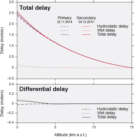
Figure 4.8. Integrated atmospheric delay (equation [4.18]) predicted by the European Centre for Medium-Range Weather Forecasts (ECMWF) ERA-40 reanalysis for two different dates in 2014 (blue: November 11, 2014; red: December 4, 2014) for a location in Albania (41.75° N; 21.75° E). For a color version of this figure, see www.iste.co.uk/cavalie/images.zip
Indeed, the typical duration of a SAR acquisition is usually of the order of approximately 1 minute (a typical integration time for a given target is of the order of approximately 1 second), whereas the revisit interval between two successive acquisitions is generally several days (six days for the Sentinel-1 system). A typical decorrelation time for zenith tropospheric delays measured by GPS is of the order of six hours, reflecting the dynamic nature of the atmospheric circulation locally (Emardson et al. 2003). Therefore, a single acquisition only captures a “snapshot” of the distribution of atmospheric heterogeneities. These features are subsequently advected and dispersed well before the next acquisition. The atmospheric artifacts resulting from this process are referred to as turbulent atmospheric artifacts. As shown in Figure 4.9, turbulent atmospheric artifacts, generally related to air moisture, are characterized by a broad spectrum of spatial correlation lengths (originating from the spatial scale of heterogeneities at any given acquisition time) but appear random in time (Hannsen 2001).
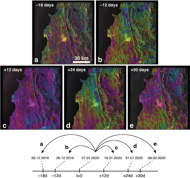
Figure 4.9. Sentinel-1 interferograms sharing the same primary acquisition over the central part of Albania. The short time span of each interferogram ensures that the fringes visible in the interferograms are primarily due to atmospheric effects, mainly caused by atmospheric turbulence. The primary acquisition was chosen for its stable atmospheric state, so that all interferograms would reflect the state of the atmosphere of the secondary acquisition. The spatially correlated nature of water vapor heterogeneity is particularly evident in (a) and (e). For a color version of this figure, see www.iste.co.uk/cavalie/images.zip
Various strategies for correcting these artifacts have been implemented. First, independent remote sensing observations of the water vapor distribution in the observed scene can be acquired by spectrometers operating in one or several absorption windows of water vapor. For instance, the MERIS instrument onboard the ENVISAT satellite, operating in visible and infrared wavelengths, allowed for mapping of the water vapor distribution at approximately 1 km spatial resolution, synchronously with the SAR acquisitions of the ASAR instrument. Using assumptions on the vertical distribution of water vapor in the column, and under cloud-free conditions, these maps could then be used to predict the wet delay in the radio domain and correct interferograms (Puysségur et al. 2007; Li et al. 2012). Unfortunately, recent SAR satellites are usually not equipped with such ancillary instruments. Alternatively, the integration of total zenithal delays routinely estimated from the analysis of GNSS data also allows for prediction of the artifacts that affect InSAR data acquired over a GNSS network (Onn and Zebker 2006). However, this approach is limited by the existence and accessibility of still scarce GNSS data and does not provide regular lateral and vertical sampling of the atmospheric column due to the constraints on the installation of GNSS stations. All these methods rely on external datasets that are not always available and for which spatial resolution generally does not compare well with that of SAR acquisitions.
Other strategies do not rely on external data. First, we can consider that interferometric delay at a given pixel depends on the pixel elevation, since the atmosphere is, to the first order, a stratified medium, as shown in Figure 4.10(a). This effect has long been recognized as a major source of uncertainty when attempting to interpret interferometric fringes in terms of ground deformation in regions characterized by large topographic features, such as volcanoes (e.g. Delacourt et al. 1998) or mountain ranges (e.g Elliott et al. 2008). The covariation between the interferometric phase and elevation is the result of the temporal variation of the altitude dependency of the atmospheric delays in equation 4.18, and, to a lesser degree, to its lateral variations. Hence, evaluating a correlation between the interferometric phase and elevation is an easy first-order correction (e.g. Cavalié et al. 2007; Jolivet et al. 2012). However, such an approach neglects local turbulent delays and can bias estimates of ground deformation if the latter also correlates with topography. Averaging of a large number of independent acquisitions, in order to cancel out these artifacts, has also been proposed. This can be achieved by stacking (thereby reinforcing any underlying steady signal, such as interseismic deformation) (Peltzer et al. 2001), performing a least-squares multi-temporal inversion (Berardino et al. 2002) or applying a low-pass temporal filter (Hooper et al. 2007). It has been shown, however, that the uneven temporal sampling of turbulent behavior and its subsequent low-pass filtering (or averaging) can lead to aliasing, which has significantly biased the estimates of ground deformation (Doin et al. 2009).
Another radically different approach consists of attempting to predict atmospheric delays using numerical weather forecast models. The rationale behind this approach relies once again on the observation that atmospheric artifacts often follow topographic features. The relation between the altitude and the delay often follows a nonlinear function, which can be empirically estimated or directly predicted from weather forecasts (Doin et al. 2009; Jolivet et al. 2011). As shown in the inset of Figure 4.10(b), for two sites located about 200 km apart, the differential delay is predicted to approximately vary linearly with elevation, but with a proportionality coefficient differing by about 30%. Mapping the predicted delays on the topography (Figure 4.10(d)) makes it possible to construct a synthetic atmospheric phase screen that can correct the observed interferogram (Figure 4.10(c)).
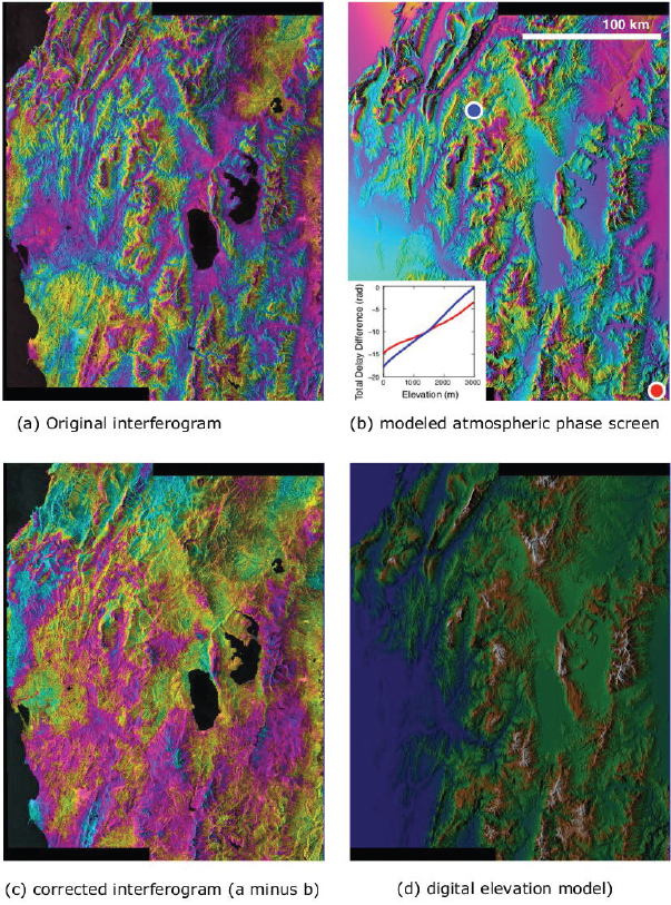
Figure 4.10. Correction of stratified tropospheric delays using the ERA-5 meteorological analysis. This Sentinel-1 interferogram covers Albania (ascending track 175; image 1: November 22, 2014; image 2: December 4, 2014). Two sub-swaths have been assembled (iw1 and iw2). The covered area is approximately 150 km wide (across-track) and 220 km long (along-track). The elevation in the scene ranges from sea level to more than 2000 m above sea level. The blue and red dots in (b) show the locations of the ERA-5 delays shown in the inset. North is at the bottom. For a color version of this figure, see www.iste.co.uk/cavalie/images.zip
The most accurate models available to describe the state of the troposphere at the relevant resolution consist of weather forecast reanalyses, which rely on the assimilation of a wealth of remote sensing and in situ meteorological observations, such as the ERA-40 and ERA-5 reanalyses of European Centre for Medium-Range Weather Forecasts (ECMWF) data (Dee et al. 2011) or the National Centers for Atmospheric Prediction (NCEP) and the National Center for Atmospheric Research (NCAR) reanalyses of National Oceanic and Atmospheric Administration (NOAA) data (Kalnay et al. 1996). In terms of temporal resolution, the ERA-5 model of the ECMWF is currently available at a one-hour resolution, which is a significant improvement compared to the six-hour resolution of the previous-generation ERA-40 reanalysis. However, these reanalyses are only available after a latency of several weeks to months. Near-real-time solutions, such as ERA-5T, or the HRES forecasts from ECMWF data, are currently considered as surrogates for correcting InSAR data for applications requiring rapid processing (Yu et al. 2018).
4.3.2. Estimation of and compensation for ionospheric propagation delays
4.3.2.1. Introduction
The ionosphere is the portion of the Earth’s upper atmosphere where ions and electrons are present with sufficient density to significantly affect the propagation of radio waves (Davies 1990). The slant total electron content (TEC) is the integrated electron density between the satellite and the target, along a tube of one square meter cross-section following the radar line-of-sight (LOS). TEC levels are higher at the equator than at higher latitudes because the ionization of the atmosphere gases depends on the solar radiation, which is stronger at lower latitudes. The activity of the sun, as well as the ionosphere, follows an 11 year cycle, with the addition of seasonal and daily variations. The most frequent perturbations of the smooth background ionosphere are equatorial and high-latitude scintillation, auroral arcs and traveling ionospheric disturbances.
The refractive index for a wave in the ionosphere is inversely proportional to its frequency, since the wave propagation speed depends on the frequency and the ionosphere is dispersive. The wave speed then needs to be distinguished into phase and group velocity, which can be shown to be equal but opposite. The main effects of the ionosphere on a traversing microwave are delay of the wave packet, advance of the phase and rotation of the polarization angle. The wave propagation in the ionosphere takes longer than in vacuum; the one-way delay is:
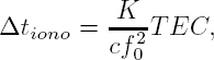
where f0 is the carrier frequency, c is the speed of light in vacuum and K = 40.28 m3/s2. While the pulse envelope is retarded, the pulse phase is advanced by the same amount:

The rotation of the polarization angle, i.e. the Faraday rotation, depends on the strength of the magnetic field B and the angle formed with the radar wave propagation vector ![]() :
:
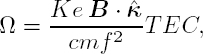
where e and m are the electron charge and mass, respectively. Additional ionospheric effects are caused by the small-scale perturbations of the ionosphere along the satellite orbit. In the azimuth direction, the synthetic aperture acts as a moving window filter. The average TEC within the aperture determines the range phase advance and group delay. The linear TEC variation shifts the focused data with respect to their correct positions by changing their zero-Doppler point. Residual nonlinear variations blur the azimuth impulse response. The nonlinear phase advance within the signal bandwidth is approximately quadratic and blurs the range impulse response. However, for typical ionospheric states and carrier frequencies higher than P-band, the blurring is minimal and can be ignored.
Ionospheric errors of many fringes and shifts of many meters can be quite common in C- and L-band interferometric and motion tracking results. It is therefore necessary to estimate and remove the ionospheric effects.
4.3.2.2. Ionosphere estimation and compensation
Absolute ionospheric levels can only be estimated with low precision from SAR data. Range blurring caused by the dispersive propagation in the ionosphere can be used to estimate the absolute TEC with very low precision (Meyer 2010). If quad-pol acquisitions are available, the Faraday rotation angle can be measured from the images and converted to a TEC value, even if the accuracy of this method is limited by the inaccurate knowledge of the magnetic field (Meyer and Nicoll 2008; Kim and Papathanassiou 2010). Alternatively, GNSS-based TEC maps can give the absolute TEC level for a SAR observation, but these values are typically biased by the very low resolution of the maps. In conclusion, a precise compensation of the errors caused by the absolute ionosphere levels, for example geolocalization or absolute motion, may not be possible.
In contrast, the compensation of differential and relative errors between SAR images is possible. The mutual ionospheric azimuth shifts can be corrected by the coregistration and resampling steps, which recover the coherence but do not separate the ground motion from the ionospheric shifts. In order to then correct the interferogram, it is necessary to estimate the ionospheric phase variation in the scene. A method that has been demonstrated to be successful is the split-spectrum method (Gomba et al. 2016, 2017). It is based on the dispersive property of the ionosphere: it can separate the ionospheric phase variation from other contributions and the estimated ionosphere can then be removed from the interferogram. Bandpass filtering of the range spectrum is used to obtain interferograms at different carrier frequencies, and then the ionospheric contribution is estimated. An example of the results of the method is shown in Figure 4.11.
Gomba and De Zan (2017) combine the split-spectrum method with the azimuth shifts estimated during the coregistration to improve the estimation results. The split-spectrum method can also be applied to a stack of images to correct the ionospheric errors in the measurement of ground motion, as demonstrated by Fattahi et al. (2017).
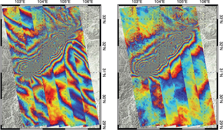
Figure 4.11. The 2008 Wenchuan Earthquake measured with ALOS interferograms, before and after applying the split-spectrum method (Gomba et al . 2016). For a color version of this figure, see www.iste.co.uk/cavalie/images.zip
4.4. InSAR processing chains
This section details the main processing steps in DInSAR processing, which are common to almost all InSAR chains (e.g. image focusing, resampling with the same acquisition geometry, common-band filtering, interferogram and coherence map generation, filtering of fringes, etc.). After discussing these key steps, we illustrate them with an earthquake case using the DiapOTB open-source software (Durand et al. 2021). A quick overview of the existing InSAR software solutions is provided at the end of this section.
4.4.1. Main steps in InSAR processing
Figure 4.12 presents the main steps in DInSAR computation.
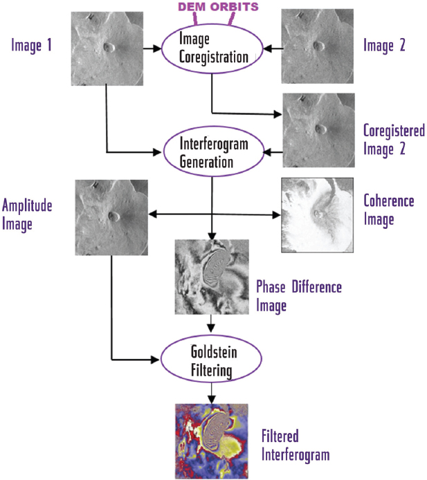
Figure 4.12. DInSAR data processing diagram with Sentinel-1 images of the Piton de la Fournaise (La Réunion, France)
4.4.1.1. Coregistration
The key step is the coregistration of the secondary image onto the reference image. The precision is a strong driver of the final coherence. For an appropriate interferogram, the coregistration should be better than a tenth of pixel.
The DEM and the orbits predict a deformation grid, which can be compared to a sparse grid obtained from local correlation with actual images: it may fail at places, revealing actual changes between images. The comparison of the two grids allows us to transfer the exact datum to the predicted distortion grid, which becomes accurate down to a few hundredths of a pixel, both locally and globally.
The primary radar image used as a reference image must be registered in absolute geographic coordinates. It is better for both images to be radar-compressed with the same SAR processor. They must share the same Doppler centroid, which should be set to the average of the optimal value found for each image.
In an ideal case of perfectly parallel orbits and aligned acquisitions, the coregistration would only need to compensate for the differing geometry due to the different viewing angle, by means of a proper cross-track stretching of one image. In practice, the coregistration should also account for orbit crossings/skewing, different sensor attitudes, different sampling rates (perhaps due to different pulse repetition frequencies (PRFs), sensor velocities, etc.) and along- and across-track shifts. The secondary image is resampled so that the final interferogram is in the same (slant-range, azimuth) reference geometry as the reference image. Range oversampling can sometimes be used in high-quality interferogram generation.
4.4.1.2. Coherence and interferogram computation
Once the two images are coregistered with the accuracy of a fraction of a pixel, the interferogram is generated by cross-multiplying pixel by pixel using the reference image with the complex conjugate of the secondary image, as previously explained in Figure 4.12.
The interferometric phase is the argument of this product or the phase difference between the images. The phase noise can be estimated from the interferometric SAR pair by means of the local coherence, which provides a useful measure of the interferogram quality (SNR). The local coherence is the cross-correlation coefficient of the SAR image pair estimated over a small window of a few pixels in range and azimuth, after the compensation for all the deterministic phase components (mainly due to the terrain elevation). The coherence map of the scene is then formed by computing the magnitude of the local coherence on a moving window that covers the whole SAR image.
4.4.1.3. Topographic fringe removal
For differential interferometry, the topographic contribution is eliminated by subtracting the fringe pattern calculated from the elevation model, removing any “predictable” fringes and leaving only those related to displacement and/or DEM improvement.
4.4.1.4. Geocoding and mosaicking
Geocoding and mosaicking are the very last steps in the interferogram generation chain, used to obtain a product in a “standard format” and to compare the results with maps and other results in the area of interest.
4.4.1.5. Filtering and unwrapping
As a final post-processing step, a Goldstein filter (Goldstein and Werner 1998) can be applied to the local interferogram power spectrum in order to increase the signal-to-noise ratio by using a fast Fourier transform on the interferogram patches. The patches are overlapped and a triangular weighted sum of the overlapping patches is used.
Most InSAR applications (e.g. topographic mapping and deformation monitoring) use the phase unwrapping approach in order to solve the 2π ambiguity in the wrapped phase (see Chapter 6).
4.4.2. Illustration of the DInSAR processing chain: a case study with DiapOTB
In this section, the earthquake that occurred on November 11, 2019, near the village of Le Teil in the Rhône River valley (Ardèche, France) is considered to illustrate the processing chain. The magnitude of the earthquake was 4.9, producing an unexpected surface rupture with ground displacement, caused by the reactivation of an ancient fault (La Rouvière) formed during an extensional tectonic period about 20–30 million years ago. Figure 4.13 show the location of Le Teil village in an IW ascending scene.
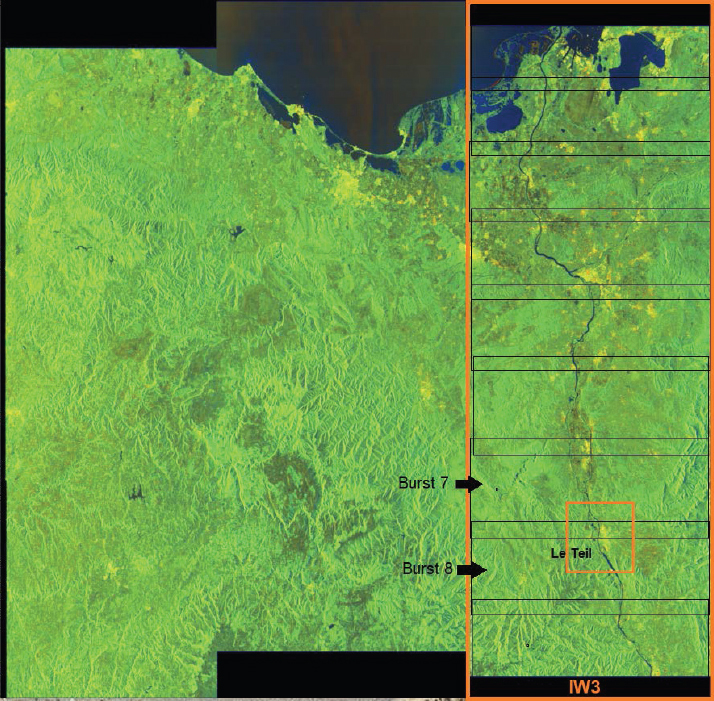
Figure 4.13. Sentinel-1 acquisition (ascending mode geometry, north is at the bottom): the Le Teil area is covered in the IW3 swath with two bursts. For a color version of this figure, see www.iste.co.uk/cavalie/images.zip
Since 2018, the new DiapOTB chain developed and provided by the CNES has offered a set of open-source filters and applications as part of the OTB. This section explains the different steps in this software, with illustrations from the Le Teil earthquake. Based on the heritage of DIAPASON, the legacy CNES interferometric processing package, DiapOTB is a complete DInSAR chain designed to work as an OTB remote module or as a stand-alone module.
DiapOTB is able to process Sentinel-1 images, both in stripmap and TOPSAR modes, and COSMO SkyMed images, both in stripmap and spotlight modes; by the end of 2021, DiapOTB will also handle TerraSAR-X and PAZ images.
4.4.2.1. Detailed description of steps in the DiapOTB chain
For the TOPSAR mode, interferometric processing is undertaken at the burst level in each DiapOTB step, as shown in the flowchart in Figure 4.14.
1) Pre-processing steps: multi-look images are produced by time-domain averaging of the SLC image samples. An independent pre-processing application is available in DiapOTB to estimate the altitude of ambiguity between a couple of images (in order to choose the best interferometric pairs). This step is not needed with Sentinel-1 images because interferometry is the main native acquisition mode (narrow orbital tube). For the TOPSAR mode, the bursts of the SLC images are extracted and a deramping function is applied (a reramping function will be needed after the final coregistration of the images before the computation of the interferogram).
2) Deformation grid for reference and other images: an accuracy better than 1/100 pixels is required for TOPSAR InSAR generation to ensure a continuous phase in the interferometric product. The slope of azimuth phase ramps induced by imperfect synchronization of reference and secondary images is proportional to the temporal lag between burst center times in the two acquisitions.
3) Coregistration of the two SLCs (secondary image onto reference geometry): for Sentinel-1 IW TOPS mode, data coregistration and DInSAR are supported.
4) Interferogram creation (a raw one or an interferogram with topographic phase suppression): for the TOPSAR mode, each interferogram is computed at the burst level and at the end recomposed at the swath level with a reramp function (an option of the deramp step). A spectral diversity method (enhanced spectral diversity (ESD)) can exploit double-difference interferograms in the burst overlap areas in order to suppress the phase discontinuities at burst edges.
5) Post-processing steps: DiapOTB includes an interferogram filtering step that uses the Goldstein method (Goldstein and Werner 1998). Terrain and ellipsoid-corrected geocoding from range-Doppler to map coordinates are included. Well-suited interpolation algorithms are applied for the resampling step. The geocoding of images in ground-range geometry is also supported.

Figure 4.14. Main DiapOTB steps for the TOPSAR processing mode. For a color version of this figure, see www.iste.co.uk/cavalie/images.zip
A python script allows the launch of the computation of interferometric time series. It includes a registration module for all the images with respect to a reference image. Then, the mean amplitude image, the interferogram and the coherence images are computed for each image pair. A DEM, from SRTM tiles, for example, overlapping the image is automatically generated and used as input. The interferograms are thus differential interferograms with respect to the DEM.
4.4.2.2. Example of processing for the Le Teil earthquake
A couple of Sentinel-1 wide interferometric images from just before and after the event, both in ascending and descending orbital directions in case of foreshortening in the area of interest, were selected and downloaded from the PEPS French portal (Figure 4.15):
S1A-IW-SLC-1SDV-20191031T173917-20191031T173944-029706-03627B-52F8.SAFE
S1A-IW-SLC-1SDV-20191112T173917-20191112T173944-029881-03689D-753A.SAFE
S1B-IW-SLC-1SDV-20191031T054322-20191031T054349-018715-023463-F95B.SAFE
S1B-IW-SLC-1SDV-20191112T054322-20191112T054349-018890-023A0A-BF8C.SAFE
The pre-earthquake image was from October 31, 2019, and the post-earthquake image was from November 12, 2019 (12 days baseline).
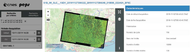
Figure 4.15. Data selection in the PEPS portal for Sentinel-1 data
DiapOTB needs metadata to process images; data must be stored in its native repositories (.SAFE for Sentinel-1 data) and formats (a tif file for Sentinel-1 data). Access to elevation data (a DEM) for the target area is also required for DInSAR processing. The DEM accuracy for the back-geocoding coregistration and terrain correction processing must be carefully chosen because phase is highly correlated with terrain topography. DiapOTB can automatically extract the required SRTM hgt tiles.
The orbit state vectors provided in the metadata of a SAR product are generally not accurate and can be refined with the precise orbit files, which are available hours to weeks after the generation of the product.
The altitude of ambiguity was estimated with the DiapOTB SARAltambig tool for the target area (latitude: 44.518, longitude: 4.671, height: 136 m), and the results led as expected to a small perpendicular baseline:
- – ascending couple: incidence angle = 43.72deg, H2π = -1375.61m, B⊥ = 11.52 m;
- – descending couple: incidence angle = 44.65deg, H2π = -256.91 m, B⊥ = 62.72 m.
Thus, the selection is suitable for DInSAR, the topography contribution will be minimized and the coherence will be convenient for InSAR results.
This example uses VV polarization images; the processing would have been the same with VH ones. The region of interest is situated in the first sub-swath, bursts 6–8 of 9. The practical run can be restricted to these bursts.
Running the DiapOTB chain involves checking (and eventually changing) the default configuration parameters for each of the steps in a .json file for the input of the DiapOTB IW python script (see https://gitlab.orfeo-toolbox.org/remote_modules/diapotb/-/wikis/ProcessingChains).
Sometimes, input processing parameters must also be defined and optimized for the InSAR image pair, depending on the sensor and the final measurement accuracy: for example, the azimuth and range multi-look factor, windows and grid sizes, etc.
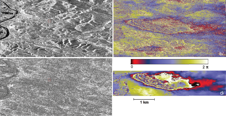
Figure 4.16. Le Teil earthquake (France, November 11, 2019): DiapOTB DInSAR raw results with SAR geometry (extracts for (a) amplitude, (b) phase before filtering, (c) coherence and (d) filtered phase) from descending Sentinel-1 acquisitions. For a color version of this figure, see www.iste.co.uk/cavalie/images.zip
The outputs of the processing are the coregistered secondary image with the same geometry as the reference image, then the raw interferogram with the three bands with SAR geometry: amplitude, phase and coherence images and the optional filtered interferogram (three bands). Figure 4.16 shows the resulting raw interferogram for the descending path with SAR geometry near Le Teil town. In Figure 4.16(c), the raw phase is still noisy. In Figure 4.16(d), the raw phase is filtered and displacement fringes appear clearly.
Figure 4.17 shows the DiapOTB results of the DInSAR processing (after Goldstein filtering and projection over the SRTM DEM tile) for a couple of Sentinel-1 images (October 31, 2019, and November 12, 2019) acquired in the two directions, from ascending and descending orbits.
We can clearly see the low coherence in the ascending path couple and thus the bad quality of the DInSAR phase image. In the area of the earthquake, the mean coherence is 0.68 (standard deviation is 0.23). The loss of coherence can be explained mainly by tropospheric artifacts (the clouds between the two acquisitions were not the same). The coherence image is much better for the descending path couple: the mean coherence is 0.89 and the standard deviation is 0.17. The fringes of the interferogram can then be analyzed by scientists.
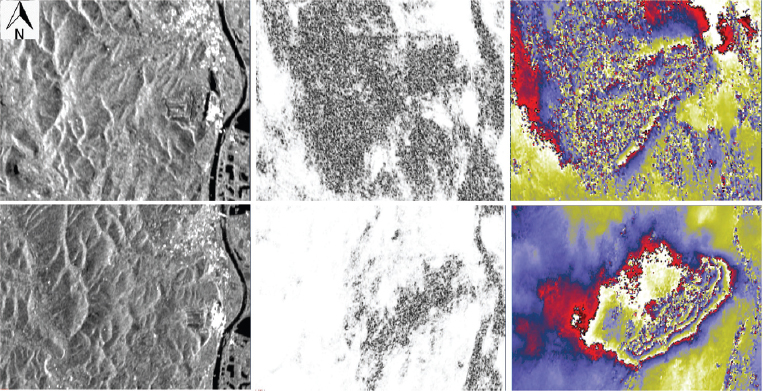
Figure 4.17. Le Teil earthquake DiapOTB DInSAR results with ground geometry (extracts for amplitude, coherence, phase from left to right) from ascending (top) and descending (bottom) Sentinel-1 acquisitions. For a color version of this figure, see www.iste.co.uk/cavalie/images.zip
Ritz et al. (2020) have reported all the analyses conducted on this earthquake. The seismological and interferometric Sentinel-1 observations indicate that the earthquake occurred at a very shallow focal depth on a southeast-dipping reverse fault. An interferogram with a good coherence (descending orbits) reveals a surface rupture and up to 15 cm uplift of the hanging wall along a northeast–southwest trending discontinuity with a length of about 5 km. Together, these lines of evidence suggest that the Oligocene La Rouvière fault was reactivated.
Figure 4.18 shows a final interferometric chart (wrapped phase) obtained using Sentinel-1 synthetic-aperture radar data pre- and post-event. This type of chart helps scientists a great deal in their geological deductions. The black lines correspond to faults after the geological map. The white line defines the about 5 km long northern section of the La Rouvière Fault (LRF) matching with the InSAR discontinuity.
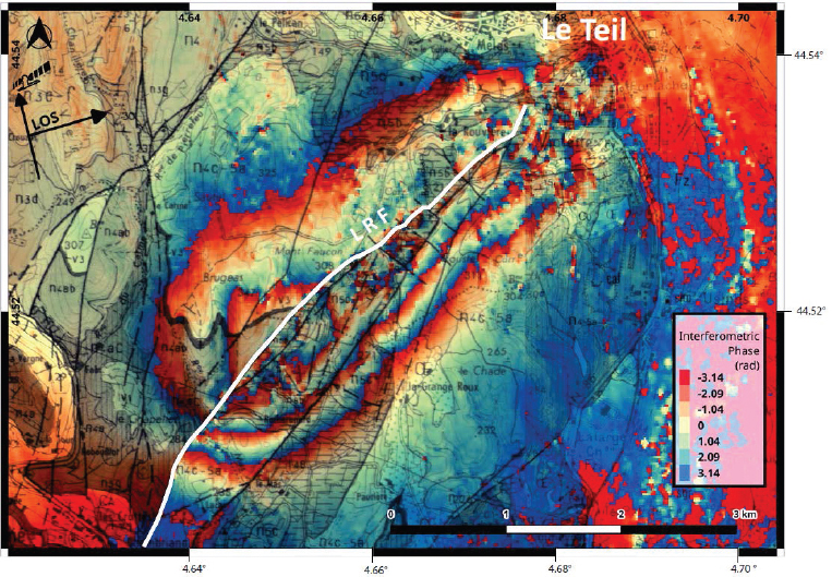
Figure 4.18. Le Teil earthquake (figure from Ritz et al . (2020)): the Sentinel-1 ascending interferogram reveals the surface rupture. For a color version of this figure, see www.iste.co.uk/cavalie/images.zip
4.4.3. Available InSAR software: a quick overview
With the large amount of freely available SLC SAR data, such as Sentinel-1 products, InSAR processing has become accessible even to non-radar specialists through the use of scientific or commercial software running automatic steps controlled by simple parameter initialization. In this section, some of the main available software packages for interferometry are listed. Some are under commercial licenses, such as GAMMA or ENVI/Sarscape; others have open licenses. Most of the free software packages for SAR interferometric processing have been developed by research institutes that work in the field of SAR interferometry. They are copyrighted and mainly for internal use, but they are also available to and shared with external SAR communities, supporting the research carried out at the respective institutes. Most of them are regularly maintained for different platforms and support new SAR mission data. The authors do not intend to advertize, nor to produce an exhaustive listing of the current InSAR software packages.
In Table 4.1, we only provide a short overview of the most current InSAR toolboxes available for the users. For more details on the software, refer to each referenced URL.
Table 4.1. Main DInSAR software packages

All the current software packages offer the entire InSAR processing chain, from SLC data to InSAR and DInSAR basic products. Some of them can undertake further steps in order to produce digital elevation models, displacement maps and land-use maps. They can include a wide range of functions – from image visualization, to DEM import and interpolation, to cartographic and geodetic transforms such as multi-looking, coregistration, despeckling, geocoding and radiometric calibration, mosaicking, feature extraction, segmentation and classification.
These chains are suited for geophysical monitoring of natural hazards such as earthquakes, volcanoes and landslides. They are also useful in structural engineering, particularly for the monitoring of subsidence and structural stability.
4.5. Conclusion
The main scientific objective of DInSAR is the characterization and quantification of underlying processes to enable the creation of predictive models that can precisely map the deformation of the Earth’s surface due to tectonic, volcanic and glacial processes. The main applications are as follows:
- – understanding strain changes leading to and following major earthquakes;
- – characterizing magma movements to predict volcanic eruptions;
- – assessing the impact of ice-sheet and glacier-system dynamics on sea level rise and characterizing temporal variability;
- – characterizing land surface motion related to subsidence, hydrology and coastal processes.
The second part of this book explains some of the InSAR applications in detail.
For surface topography mapping, a pre-existing digital elevation model (DEM) can be used. With a slight difference in radar position, changes in topography cause a distortion in the phase, much like a stereographic image. Using the known baseline distance, the height of the surface can be derived from multiple observations and a DEM created. The topography can then be corrected, and the phase and the image pixels rearranged to correspond to latitude and longitude in order to produce a correct “geocoded” projection.
When the contributions to the signal’s phase of the ground surface, orbital effects and topography are removed, what remains in the image is the change in surface movement or deformation. Differential InSAR is not a tool for accurate pixelic local displacement measurements, but it is useful in monitoring progressing movements over large areas. With regard to the identification of linear and nonlinear deformation patterns and the abillity to follow time histories of movement for every radar target of a large dataset, a significant development of conventional InSAR is the use of permanent scatterer interferometry (PSI), as explained in the next chapter dedicated to multi-temporal InSAR approaches.
4.6. Acknowledgments
The authors thank Raphaël Grandin and Romain Jolivet for writing section 4.3.1 and Jean-Marie Nicolas for the careful review and comments that helped to improve this chapter.
4.7. References
Baby, H.B., Gole, P., Lavergnat, J. (1988). A model for the tropospheric excess path length of radio waves from surface meteorological measurements. Radio Science, 23, 1023–1038.
Berardino, P., Fornaro, G., Lanari, R., Sansosti, E. (2002). A new algorithm for surface deformation monitoring based on small baseline differential SAR interferograms. IEEE Transactions on Geoscience and Remote Sensing, 40, 2375–2383.
Cavalié, O., Doin, M.-P., Lasserre, C., Briole, P. (2007). Ground motion measurement in the Lake Mead Area, Nevada, by differential synthetic aperture radar interferometry time series analysis: Probing the lithosphere rheological structure. Journal of Geophysical Research: Solid Earth, 112(B3), 1–18.
Davies, K. (1990). Ionospheric Radio. IET, London.
Dee, D.P., Uppala, S.M., Simmons, A., Berrisford, P., Poli, P., Kobayashi, S., Andrae, U., Balmaseda, M., Balsamo, G., Bauer, D.P. et al. (2011). The ERA-Interim reanalysis: Configuration and performance of the data assimilation system. Quarterly Journal of the Royal Meteorological Society, 137(656), 553–597.
Delacourt, C., Briole, P., Achache, J. (1998). Tropospheric corrections of SAR interferograms with strong topography. Application to Etna, 25, 2849–2852.
Doin, M.-P., Lasserre, C., Peltzer, G., Cavalié, O., Doubre, C. (2009). Corrections of stratified tropospheric delays in SAR interferometry: Validation with global atmospheric models. Journal of Applied Geophysics, 69(1), 35–50.
Durand, P., Pourthié, N., Tison, C., Usseglio, G. (2021). DiapOTB: A new open source tool for differential SAR interferometry. EUSAR On Line Conference, 29 March–1 April.
Elliott, J.R., Biggs, J., Parsons, B., Wright, T.J. (2008). InSAR slip rate determination on the Altyn Tagh Fault, northern Tibet, in the presence of topographically correlated atmospheric delays. Geophysical Research Letters, 35.
Emardson, T.R., Simons, M., Webb, F.H. (2003). Neutral atmospheric delay in interferometric synthetic aperture radar applications: Statistical description and mitigation. Journal of Geophysical Research, 108(B5), 1–8.
Fattahi, H., Simons, M., Agram, P. (2017). InSAR time-series estimation of the ionospheric phase delay: An extension of the split range-spectrum technique. IEEE Transactions on Geoscience and Remote Sensing, 55(10), 5984–5996.
Fjortoft, R., Gaudin, J., Pourthié, N., Lalaurie, J., Mallet, A., Nouvel, J., Martinot-Lagarde, J., Oriot, H., Borderies, P., Ruiz, C., Daniel, S. (2014). KaRIn on SWOT: Characteristics of near-nadir Ka-band interferometric SAR imagery. IEEE Transactions on Geoscience and Remote Sensing, 52(4), 2172–2185.
Fornaro, G. and Guarnieri, A.M. (2002). Minimum mean square error space-varying filtering of interferometric SAR data. IEEE Transactions on Geoscience and Remote Sensing, 40(1), 11–21.
Goldstein, R. and Werner, C. (1998). Radar interferogram filtering for geophysical applications. Geophysical Research Letters, 25(21), 4035–4038.
Gomba, G. and De Zan, F. (2017). Bayesian data combination for the estimation of ionospheric effects in SAR interferograms. IEEE Transactions on Geoscience and Remote Sensing, 55(11), 6582–6593.
Gomba, G., Parizzi, A., De Zan, F., Eineder, M., Bamler, R. (2016). Toward operational compensation of ionospheric effects in SAR interferograms: The split-spectrum method. IEEE Transactions on Geoscience and Remote Sensing, 54(3), 1446–1461.
Gomba, G., Gonzalez, F.R., De Zan, F. (2017). Ionospheric phase screen compensation for the Sentinel-1 TOPS and ALOS-2 ScanSAR modes. IEEE Transactions on Geoscience and Remote Sensing, 55(1), 223–235.
Hannsen, R.F. (2001). Radar Interferometry: Data Interpretation and Error Analysis. Springer-Verlag, Heidelberg.
Hooper, A., Segall, P., Zebker, H.A. (2007). Persistent scatterer interferometric synthetic aperture radar for crustal deformation analysis, with application to Volcán Alcedo, Galápagos. Journal of Geophysical Research: Solid Earth, 112(B7), 1–21.
Jolivet, R., Grandin, R., Lasserre, C., Doin, M.P., Peltzer, G. (2011). Systematic InSAR tropospheric phase delay corrections from global meteorological reanalysis data. Geophysical Research Letters, 38(17), 1–6.
Jolivet, R., Lasserre, C., Doin, M.-P., Guillaso, S., Peltzer, G., Dailu, R., Sun, J., Shen, Z.-K., Xu, X. (2012). Shallow creep on the Haiyuan Fault (Gansu, China) revealed by SAR interferometry. Journal of Geophysical Research: Solid Earth, 117(B6), 1–8.
Kalnay, E., Kanamitsu, M., Kistler, R., Collins, W., Deaven, D., Gandin, L., Iredell, M., Saha, S., White, G., Woollen, J. et al. (1996). The NCEP/NCAR 40-year reanalysis project. Bulletin of the American Meteorological Society, 77(3), 437–472.
Kim, J.S. and Papathanassiou, K.P. (2010). Faraday rotation estimation performance analysis. 8th European Conference on Synthetic Aperture Radar (EUSAR), Aachen.
Lazecky, M., Bakon, M., Hlavacova, I. (2015). Effect of DEM inaccuracy on precision of satellite InSAR results. GIS Ostrava Conference, Ostrava.
Li, Z., Xu, W., Feng, G., Hu, J., Wang, C., Ding, X., Zhu, J. (2012). Correcting atmospheric effects on InSAR with MERIS water vapour data and elevation-dependent interpolation model. Geophysical Journal International, 189(2), 898–910.
Massonnet, D. (1997). Producing ground deformation maps automatically: The diapason concept. IEEE International Geoscience and Remote Sensing Symposium, 3–8 August, Singapore.
Massonnet, D. and Feigl, K.L. (1995). Discrimination of geophysical phenomena in satellite radar interferograms. Geophysical Research Letters, 22(12), 1537–1540.
Meyer, F. (2010). A review of ionospheric effects in low-frequency SAR – Signals, correction methods, and performance requirements. Geoscience and Remote Sensing Symposium, 25–30 July.
Meyer, F. and Nicoll, J. (2008). Prediction, detection, and correction of Faraday rotation in full-polarimetric L-band SAR data. IEEE Transactions on Geoscience and Remote Sensing, 46(10), 3076–3086.
Onn, F. and Zebker, H.A. (2006). Correction for interferometric synthetic aperture radar atmospheric phase artifacts using time series of zenith wet delay observations from a GPS network. Journal of Geophysical Research: Solid Earth, 111(B9), 1–16.
Peltzer, G., Crampé, F., Hensley, S., Rosen, P. (2001). Transient strain accumulation and fault interaction in the Eastern California shear zone. Geology, 29, 975–978.
Prats-Iraola, P., Rodriguez-Cassola, M., Zan, F.D., Scheiber, R., Lopez-Dekker, P., Barat, I., Geudtner, D. (2015). Role of the orbital tube in interferometric spaceborne SAR missions. IEEE Geoscience and Remote Sensing Letters, 12(7), 1486–1490.
Puysségur, B., Michel, R., Avouac, J.-P. (2007). Tropospheric phase delay in interferometric synthetic aperture radar estimated from meteorological model and multispectral imagery. Journal of Geophysical Research Solid Earth, 112(B11), B05419.
Ritz, J., Baize, S., Ferry, M., Larroque, C., Audin, L., Delouis, B., Mathot, E. (2020). Surface rupture and shallow fault reactivation during the 2019 Mw 4.9 Le Teil earthquake, France. Communications Earth and Environment, August, 1(10).
Rosen, P., Hensley, S., Joughin, I., Li, F., Madsen, S., Rodriguez, E., Goldstein, R. (2000). Synthetic aperture radar interferometry. Proceedings of the IEEE, 88, 333–382.
Tupin, F., Inglada, J., Nicolas, J.-M. (2014). Remote Sensing Imagery. ISTE Ltd, London, and Wiley, New York.
Yu, C., Li, Z., Penna, N.T., Crippa, P. (2018). Generic atmospheric correction model for interferometric synthetic aperture radar observations. Journal of Geophysical Research: Solid Earth, 123(10), 9202–9222.
Zebker, H.A., Rosen, P.A., Hensley, S. (1997). Atmospheric effects in interferometric synthetic aperture radar surface deformation and topographic maps. Journal of Geophysical Research: Solid Earth, 102(B4), 7547–7563.
- 1. A DEM is a model providing knowledge of the ground terrain, a “bare Earth” elevation model, on a geolocalized regular grid, unmodified from its original data source, which is in theory free of vegetation, buildings and other “non-ground” objects (generic term for a superset including both a digital terrain model (DTM) and digital surface model (DSM) with objects), but which in practice has some artifacts. A DEM is a digital image in which each pixel has a value corresponding to its altitude above sea level. It can be derived by digitizing elevation data from topographic maps or, directly, from stereo imagery, interferometric synthetic aperture radar or light detection and ranging (LiDAR).