
3
SAR Offset Tracking
Silvan LEINSS1,2 , Shiyi LI1, Yajing YAN2 and Bas ALTENA3
1Institute of Environmental Engineering, ETH Zurich, Switzerland
2LISTIC, Savoie Mont Blanc University, Annecy, France
3IMAU, Utrecht University, The Netherlands
In order to provide the basics for the different image correlation methods used for SAR offset tracking, we start with a brief introduction to the SAR imaging geometry and the imaging method and provide a description of radar speckle. Then, we explain various methods of SAR image correlation, followed by two advanced methods using SAR image time series to make offset tracking more robust against decorrelation. We conclude this chapter with the fusion of displacement observations from different orbits into three-dimensional displacement maps.
3.1. Basics of SAR imaging
3.1.1. Imaging geometry and resolution of SAR systems
Synthetic aperture radar (SAR) systems illuminate the scene sideways with a broad antenna beam and sample the backscattered signal at different slant-range distances R (Figure 3.1). The measurement is repeated at different positions along the flight direction (satellite orbit), defining the second image dimension, named the azimuth. Except for interferometric systems, radar systems cannot measure the exact direction (look angle θ) at which the scene is observed. Complementary to radar systems, optical systems can only measure the direction in which radiation is emitted and, except for lidar systems, distances cannot be measured. With this perspective, the slant-range imaging of radar systems can be considered as orthogonal to the imaging geometry of an optical system.
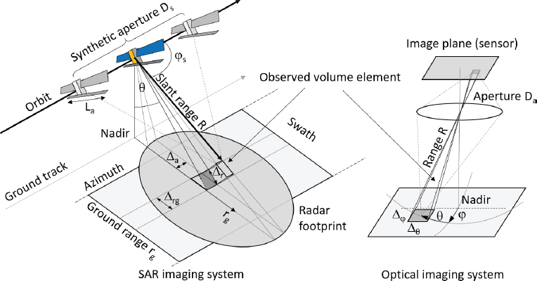
Figure 3.1. SAR imaging geometry compared to the imaging geometry of a simple optical system. The radar system samples the scene in azimuth and slant-range coordinates (R) and cannot measure the illumination angle θ. The optical system samples the scene in 2D angular coordinates (θ,ϕ ) but cannot measure the (slant) range R. For a color version of this figure, see www.iste.co.uk/cavalie/images.zip
The orientation of the slant-range and azimuth direction is given by the satellite’s orbit. To image nearly every part of the Earth as they rotate underneath satellites, and because SAR systems require several kW of electrical power, all spaceborne radar sensors fly in a near-polar, sun-synchronous dusk–dawn orbit (see Chapter 1, section 1.1.1), where solar panels can always be illuminated by the sun. This makes the azimuth direction roughly aligned with the north/south direction (inclination ≈ 98°) and results in overpass times at early morning and early evening. The orbit of a satellite moving from the south to the north is called the ascending orbit, whereas it is called the descending orbit when the satellite moves from the north to the south (Figure 3.2). Considering that most SAR systems use a right-looking imaging geometry with respect to the flight direction (azimuth), SAR sensors look approximately towards the east from ascending orbits and approximately towards the west from descending orbits.
SAR systems can provide high-resolution imagery through range and azimuth compression of the received, unfocused, raw backscatter signal (Olmsted 1993; Oliver and Quegan 2004). After compression (focusing), a radar pixel (resolution cell) represents all power scattered back from objects located at a certain range and azimuth, defined by the volume element shown in Figure 3.1. Similar to optical systems, where the diameter Da of the aperture lens limits the imaging resolution, the length of the synthetic aperture Ds of the radar system limits the azimuth resolution (Figure 3.1). Within the synthetic aperture, an object is illuminated by the antenna beam. The width of the antenna beam is diffraction-limited and depends on the length La of the radar antenna (the real aperture). As the opening angle of the illuminating antenna beam does not depend on distance, the azimuth resolution Δa is independent of the distance. In theory, the azimuth resolution for the stripmap imaging mode is only given by the antenna length: Δa ≈ La/2. In practice, signal power, pulse repetition frequency, azimuth ambiguities, etc., limit the azimuth resolution to values somewhat larger than La/2. In the slant-range direction, the resolution Δr ≈ BR/(2c) is given by the inverse of the radar bandwidth BR and the speed of light c. After focusing, the spatial resolution, or more precisely, the size of the radar resolution cell, is given by the slant-range resolution Δr and the azimuth resolution Δa (see also Chapter 1, section 1.1.2).
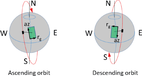
Figure 3.2. Look-and-flight directions (black and red arrows) for SAR acquisitions from ascending and descending orbits. For a color version of this figure, see www.iste.co.uk/cavalie/images.zip
Most modern SAR sensors have polarimetric imaging capabilities, either as a default mode (e.g. Sentinel-1) or as optional modes (e.g. TerraSAR-X). The geometric and radiometric resolution as well as the noise floor of acquisitions depends on the system design, but they can be lower for dual- or quad-polarimetric modes. Therefore, single-polarization acquisitions are often preferred for offset tracking.
As SAR images are generated by measuring distances, an oblique imaging geometry is required to obtain a good spatial resolution of the observed scene. However, the resolution depends on the terrain slope. For a horizontal terrain, the ground-range resolution Δrg = Δr/ sin θinc is given by projecting the slant-range resolution Δr to the ground (Figure 3.3). The local incidence angle θinc is defined with respect to the vertical. For mountainous terrain, the slope of the local topography can be defined by the angle ζ, measured in the slant-range plane, perpendicular to the azimuth direction. In this plane, a positive slope, ζ > 0, faces the radar and a negative slope, ζ < 0, faces away from the radar. The spatial resolution, parallel to the slope, is then given by
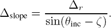
The best resolution is obtained for a slope-parallel incident beam (θinc − ζ = 90°). Steeper slopes, which face away from the radar and cannot be illuminated, are located in the radar shadow (dark gray in Figure 3.3). For slopes facing the radar, the denominator in equation [3.1] approaches zero at ζ = θinc, where all resolution is lost. For steeper slopes, multiple areas on the terrain exist that have the same distance to the radar. The backscatter signals of these areas overlap; hence, they are imaged into the same radar pixel. This situation is called the radar layover or foldover. With increasing incidence angles, the extent of shadow increases while the extent of layover decreases. For mountaineous terrain, incidence angles minimizing the extent of shadow and layover are in the range of 45–55 degrees.
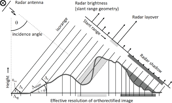
Figure 3.3. Sampling of the topography in slant-range coordinates. The x-axis indicates the effective resolution on the ground. The areas with the same range fall into layover (light gray). The areas in the radar shadow (dark gray) cannot be imaged. The image was redrawn from Rosen et al . (2000)
Figure 3.4(a) shows an example of a real SAR image with radar coordinates, acquired over the Great Aletsch Glacier (Switzerland) from a descending orbit. In this figure, strong geometric distortions appear because of the oblique, slant-range imaging geometry. Mountains appear distorted or even folded over lower terrain (layover) and point towards the sensor on the right side of the image. Layover appears as bright but narrow ridges, and radar shadow appears on the west-facing mountain slopes in black. Orthorectification alters the pixel spacing (see also Figure 3.3) and projects the image into a planar map geometry (Figure 3.4b); slopes facing away from the sensor appear compressed, while slopes facing the radar get stretched over larger areas. The areas affected by shadow or layover are indicated in blue and red in the shaded relief (Figure 3.4(c)). Orthorectification is performed using a lookup table for interpolation, which is based on the orbit information and an external digital elevation model (DEM).
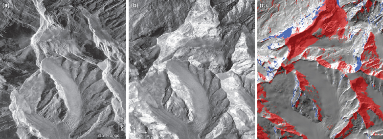
Figure 3.4. (a) Great Aletsch Glacier (Switzerland) imaged in the slant-range geometry from a descending orbit (TerraSAR-X, ©DLR 2021; incidence angle θ = 32°). (b) Orthorectified radar image. (c) Shaded relief with masks for layover (red) and radar shadow (blue). For a color version of this figure, see www.iste.co.uk/cavalie/images.zip
3.1.2. Radar speckle and speckle reduction with multi-looking
Almost all radar imagery is affected by radar speckle, which can make imagery appear very noisy. The speckle pattern is temporally variable and depends on the surface characteristics. It can either hide or provide information required for displacement measurements. Therefore, we provide here a brief introduction to radar speckle.
Speckle originates from interference. Both ways of image formation, the focusing of light with a lens and the focusing of microwaves with a synthetic aperture, are based on the fact that radiation scattered at a point of the observed scene is collected by an aperture and is then superposed at a location on the image sensor (by a lens for the optical system) or at a slant-range azimuth location in the SAR image (focused numerically). For the two methods, the superposition of radiation generates an interference pattern at the detector. However, during the exposure time of optical systems, the interference pattern is averaged out in time because natural light has a very short temporal coherence. The radar microwave pulses, however, are identical copies of each other and hence temporally coherent. When all the radiation received during the synthetic aperture is superimposed by focusing, the full interference pattern of scattered amplitudes appears in the radar pixels. Notably, SAR systems measure complex-valued backscatter amplitudes containing phase information, whereas optical systems can only measure intensity.
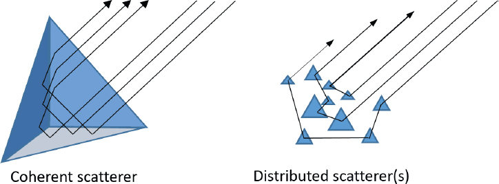
Figure 3.5. The scattering amplitude and phase of a coherent target is independent of the exact location where scattering occurs; they can appear very bright. The scattering from distributed targets is described by random sum-scattered amplitudes resulting in radar speckle
The interference pattern measured by the SAR system depends on the observed target. For coherent scatterers, such as corner reflectors of “sheet metal” (left side in Figure 3.5), all scattered microwaves interfere constructively because they have exactly the same travel time. This makes such targets appear very bright with a well-defined scattering amplitude and phase. In contrast, natural surfaces can be described by an ensemble of many small distributed scatterers. The backscatter amplitudes of all these scatterers sum up coherently and form the measured signal of the distributed objects. The amplitude A and phase φ of the corresponding pixel of a single-look complex (SLC) radar image can then be written as a sum of random complex numbers (Oliver and Quegan 2004). For the expectation value of the backscatter intensity I = |A|2, it can be shown that the standard deviation of every speckle-affected backscatter estimate is equivalent to its mean, or, in other words, every measurement has an uncertainty of 100% (Oliver and Quegan 2004). This is why SAR images of natural surfaces are characterized by granular or “salt and pepper” textures, as is visible in Figure 3.6(a). The effect is known as radar speckle, commonly also referred to as speckle noise due to the noise-like appearance.
Speckle makes the interpretation of radar images difficult and can hide trackable features. To improve interpretation, incoherent averaging of multiple intensity measurements can be applied to obtain a better estimate of the local intensity I. While the expectation value ‹I› of the intensity remains the same, the standard deviation is given by ![]() Here, L represents the number of independent measurements or “looks” at the scene, and therefore this process is called multi-looking. There are various methods to generate a multi-looked SAR image, but the most common method is spatially averaging the backscatter intensity, assuming that adjacent pixels represent similar types of scattering (looks at adjacent pixels, ensemble average). This, however, results in a loss of spatial details (Figure 3.6(b)). In contrast, averaging of a number of radar images acquired at different times (temporal multi-looking) can greatly enhance the visibility of stable, non-moving details in the scene. Unfortunately, temporal information is lost and moving surfaces show motion blur (Figure 3.6(c)). Despite the reduction of speckle, the loss of spatial or temporal resolution in multi-looked radar images can deteriorate the precision of tracking.
Here, L represents the number of independent measurements or “looks” at the scene, and therefore this process is called multi-looking. There are various methods to generate a multi-looked SAR image, but the most common method is spatially averaging the backscatter intensity, assuming that adjacent pixels represent similar types of scattering (looks at adjacent pixels, ensemble average). This, however, results in a loss of spatial details (Figure 3.6(b)). In contrast, averaging of a number of radar images acquired at different times (temporal multi-looking) can greatly enhance the visibility of stable, non-moving details in the scene. Unfortunately, temporal information is lost and moving surfaces show motion blur (Figure 3.6(c)). Despite the reduction of speckle, the loss of spatial or temporal resolution in multi-looked radar images can deteriorate the precision of tracking.

Figure 3.6. Radar image of a glacier (left side) flowing around a rock ridge (right side). (a) The single-look backscatter intensity is strongly affected by speckle. (b) Speckle reduction using spatial multi-looking with a 5x5 pixel Gaussian smoothing kernel blurs the image. (c) Speckle reduction using temporal multi-looking from 10 consecutive images (repeat interval: 11 days) reveals details on the rock, but causes motion blur on the glacier. Images by TerraSAR-X (©DLR 2021)
For SAR offset tracking, the intensity distribution of measured backscatter values is relevant. It can be shown that the measured intensity I can be written as σn, where n is a multiplicative term, carrying all random speckle noise, and σ is the true backscatter value (Oliver and Quegan 2004). It follows that speckle is exponentially distributed with Pn(n) = e−n with n > 0, and that every measurement can be regarded as its true backscatter value σ multiplied by the speckle noise n, which has a mean value ![]() The multiplicative nature of speckle makes it possible to separate the noise from the expectation value σ by considering the log of the measured intensity, commonly done by transforming the intensity I to decibels (dB):
The multiplicative nature of speckle makes it possible to separate the noise from the expectation value σ by considering the log of the measured intensity, commonly done by transforming the intensity I to decibels (dB):
Applying the log on the intensity compresses the (exponential) dynamic range of the image and standardizes the noise, which makes it independent of the mean value σ (Oliver and Quegan 2004). This can improve the cross-correlation because features with a relatively low backscatter intensity gain more weight in the correlation.
Finally, for very temporally stable surfaces, the speckle pattern can show temporal coherence such that either the complex radar image or its magnitude can be used as input for offset tracking. Furthermore, strong persistent scatterers that outshine the speckle pattern (radar reflector, Figure 3.5) can be used as trackable point-like targets. For very high resolution radar sensors, speckle can be reduced or even made almost absent when only a very limited number of scatterers are present in each resolution cell.
3.1.3. Spectral support of the backscatter intensity
When calculating the intensity from the SLC amplitude, it should be kept in mind that radar images are bandwidth-limited images and that the spectrum of the intensity requires double spectral support (Werner et al. 2005). To illustrate this, Figure 3.7 shows the typical spectrum of an SLC radar image (black line). The shape of the spectrum is defined by a hamming window, which is used to reduce side lobes of very bright scatterers. The spectrum shown requires a slightly smaller spectral support than twice the Nyquist frequency fN because the SLC data are slightly oversampled. The spatial sampling frequency of the data shown is given by 1/(2fN).
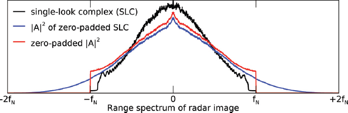
Figure 3.7. The slant-range spectrum of the single-look-complex amplitude image (black) requires half of the spectral support of the intensity (blue) computed by zero-padding the SLC. In the spectrum of the intensity computed without zero-padding the SLC (red), the wings of the blue curve are folded into the spectral range between the Nyquist frequencies of the SLC image ±fN , which deteriorates the image quality. For a color version of this figure, see www.iste.co.uk/cavalie/images.zip
When calculating the intensity of image components, for which the amplitude shows a spatial variation faster than half the Nyquist frequency, I = |A(t)|2 = ![]() it becomes clear that the frequency doubles; this is why the intensity requires double spectral support to avoid aliasing (blue line in Figure 3.7). For SAR data, oversampling is performed by zero-padding the Fourier transform of the image to double the spectral bandwidth, and then applying an inverse Fourier transform before calculating the backscatter intensity (De Zan 2014). This oversampling of the (complex-valued) amplitude can enhance the precision of offset tracking. In practice, and as shown in Figure. 3.7, SAR data are often already slightly oversampled and the spectral weighting with a hamming window reduces high-frequency components of the images, which can make oversampling superfluous. Nevertheless, to attain good sub-pixel precision, oversampling of the complex amplitude before correlating the intensity is more reasonable than oversampling the intensity (red line in Figure 3.7).
it becomes clear that the frequency doubles; this is why the intensity requires double spectral support to avoid aliasing (blue line in Figure 3.7). For SAR data, oversampling is performed by zero-padding the Fourier transform of the image to double the spectral bandwidth, and then applying an inverse Fourier transform before calculating the backscatter intensity (De Zan 2014). This oversampling of the (complex-valued) amplitude can enhance the precision of offset tracking. In practice, and as shown in Figure. 3.7, SAR data are often already slightly oversampled and the spectral weighting with a hamming window reduces high-frequency components of the images, which can make oversampling superfluous. Nevertheless, to attain good sub-pixel precision, oversampling of the complex amplitude before correlating the intensity is more reasonable than oversampling the intensity (red line in Figure 3.7).
3.1.4. Offsets due to radar penetration
Radar images are generated by measuring the distance to an observed surface. However, this distance is not necessarily the geometric distance to a metallic target, and atmospheric delays and penetration into the observed medium can result in an apparent shift of the observed surface. These may be (seasonal) height changes due to a varying radar penetration into vegetation or snow or sand appearing as a slant-range displacement. Furthermore, the surface accumulation of snow or ablation (e.g. snow fall, ice melt) can result in slant-range shifts, which might be misinterpreted as displacement (Leinss and Bernhard 2021). This needs to be kept in mind when interpreting generated displacement maps.
3.2. SAR offset tracking
Offset tracking originates from image registration methods. Lucchitta and Ferguson (1986) visually inspected time series of Landsat imagery and found persistent features on outlet glaciers in Antarctica which could be manually tracked. Bindschadler and Scambos (1991) used the high sensitivity of the human eye (optical flow) and flickered consecutive Landsat imagery on a computer screen to identify shifts in the low-frequency undulation field of an ice stream in Antarctica. They used these shifts for coregistration of the images and then applied two methods on the high-pass filtered images: a manual point-picking method to track features and a numerical cross-correlation method to match patterns in a reference area with patterns from a search area. Scambos et al. (1992) provide the details of the method and use image-to-image cross-correlation software applied on small templates of an image pair. For SAR imagery, offset tracking originates from SAR interferometry, which requires the precise coregistration of two SAR images to obtain interferometric coherence and fringe visibility (see section 4.4.1.1.). However, while with SAR interferometry only slant-range displacement can be measured, Gray et al. (1998) showed that radar speckle can be tracked in the slant range and azimuth direction with cross-correlation. In the following sections, we first describe the method of offset tracking using cross-correlation in detail and then describe various variants of cross-correlation with SAR data.
3.2.1. Cross-correlation
3.2.1.1. Cross-correlation in the spatial domain
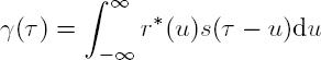
Cross-correlation is a commonly used similarity measure in signal processing. Given a reference signal r(t) and a search signal s(t), the cross-correlation between the two signals can be defined as a function of the shift τ of s relative to r:
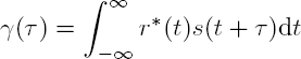
with r∗(t) being the complex conjugate of r. Equation [3.3] expresses the cross-correlation for a 1D continuous signal. Considering images as discrete signals sampled in 2D space, equation [3.3] can be rewritten as:
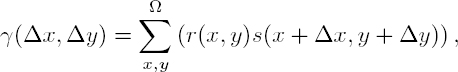
with (x, y) being the image coordinates, (Δx, Δy) the image shifts and Ω the domain of the image templates, i.e. the size of the correlation window. Equation [3.4] would result in strongly varying values for γ for areas of different brightness in the images. To make the correlation values of different image areas comparable, the image templates need to be adjusted by their mean values μr, μs and normalized by their standard deviation, which results in the normalized cross-correlation (NCC):
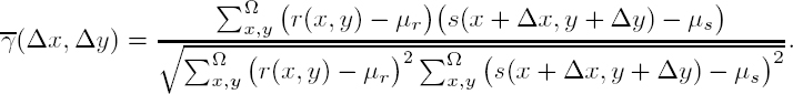
The numerator of equation [3.5] is scaled by 1/N (N defines the total number of pixels in the template domain Ω) and thus cancels out the 1/N in the standard deviation of the templates. The values of the NCC range between ![]() and the maximum cp of the cross-correlation peak is also called the normalized cross-correlation coefficient.
and the maximum cp of the cross-correlation peak is also called the normalized cross-correlation coefficient.
The location of the maximum of ![]() provides an estimate of the offset
provides an estimate of the offset ![]() between the image templates. Oversampling of the input data r, s and interpolation or curve-fitting of the cross-correlation peak (a brief overview is given by Tong et al. (2019)) allows for tracking with sub-pixel accuracy with different levels of precision (Debella-Gilo and Kääb 2011). However, depending on the method used, “pixel-locking” or “peak-locking” can occur, i.e. the probability that integer offsets are determined by peak-fitting is higher than non-zero sub-pixel offsets (Chen and Katz 2005).
between the image templates. Oversampling of the input data r, s and interpolation or curve-fitting of the cross-correlation peak (a brief overview is given by Tong et al. (2019)) allows for tracking with sub-pixel accuracy with different levels of precision (Debella-Gilo and Kääb 2011). However, depending on the method used, “pixel-locking” or “peak-locking” can occur, i.e. the probability that integer offsets are determined by peak-fitting is higher than non-zero sub-pixel offsets (Chen and Katz 2005).
3.2.1.2. Confidence measure of offset estimation
An offset can only be reliably estimated by unambiguously identifying the cross-correlation peak. To quantify the confidence of offset estimation, two parameters are often used: the normalized cross-correlation value (height of the correlation peak) cp and the signal-to-noise ratio (SNR) of the cross-correlation. Higher confidence is normally characterized by a higher correlation peak cp, but multiple peaks can exist when periodic patterns are present in the images. The SNR is usually defined as the ratio between the height of the NCC peak and the average of the ambient correlation field ![]()
A high SNR indicates a high likelihood that a unique peak is present in the cross-correlation, whereas a low SNR can either be related to strong noise in the cross-correlation or to periodic patterns showing multiple peaks of high correlation cp. Further methods exist to improve the confidence in the estimated offset (see Chapter 11, section 11.3.4.1).
3.2.1.3. Cross-correlation in the frequency domain
The direct calculation of the cross-correlation in the spatial domain is computationally expensive, especially for the relatively large templates required for SAR data as the computational time scales with the number of pixels per template. To reduce the computational complexity, we can calculate the cross-correlation in the frequency domain. For equation [3.3], flipping r∗(t) as r∗(−t) and letting u = −t, we have
which is a convolution integral. Using the convolution theorem, which states that the Fourier transform of a convolution is identical to the product of the two spectra
with · being element-wise multiplication, we can calculate the normalized cross-correlation in the frequency domain as

with F {r} and F {s} being the (fast) Fourier transformation of the two templates, and |F {. . . } |2 the total of the power spectrum of r and s. Here, we used F {r∗} = F {r}∗. The frequency-domain correlation ![]() can be transformed back through the inverse Fourier transformation
can be transformed back through the inverse Fourier transformation ![]() to track the cross-correlation peak in the spatial domain.
to track the cross-correlation peak in the spatial domain.
3.2.1.4. Sub-pixel estimation in the frequency domain
Displacements can not only be determined by sub-pixel localization of the cross-correlation peak but also directly from the cross-correlation in the frequency domain. When an integer shift is present and the phase-correlation matrix (see section 3.2.2.4) is transformed back to the spatial domain, the resulting correlation surface will be a unit impulse. However, to ensure the discrete nature of the Fourier transform, the impulse is diluted (or convoluted) by a 2D sinc, which smears most of the energy to immediate adjacent neighbors, but surrounded by steep dips (Foroosh et al. 2002). Thus, peak-locking effects appear (Chen and Katz 2005).
In order to estimate displacements through frequency methods, it is beneficial to directly estimate them in the phase plane. The phase values in the cross-spectrum have a saw-tooth pattern, where the ridges align perpendicular to the direction of the displacement, and the number of cycles corresponds to the magnitude of the displacement. Hence, many algorithms use unwrapping or work out a solution along one axis (see Balci and Foroosh (2006)). Along two axes, the Radon transform, random sample consensus (RANSAC) or single value decomposition (SVD) can also be used (see a review in Tong et al. (2019)).
Alternatively, a two-step procedure can be used, where the integer displacement is first estimated. This integer step is used to realign the template. Then, the displacement is below one pixel displacement and the saw tooth can be approximated by a plane, making direct estimation possible (Stone et al. 2001; Hoge 2003) or easing the convergence of iteration (Leprince et al. 2007). Phase-plane fitting is well-established using optical imagery. However, its application on SAR data is a current topic of research because the high-frequency noise from SAR speckle makes the application of phase correlation difficult.
3.2.2. SAR offset tracking using image pairs
Equations [3.5] and [3.7] are widely used for offset tracking with optical and SAR imagery. Depending on the speckle statistics of the SAR images, different types of input information are used for the templates r and s, and thus different sub-types of SAR offset tracking are described in the following, including coherence tracking, speckle tracking and intensity tracking.
3.2.2.1. Coherence tracking
For coherence tracking, the single-look-complex values Aejφ of a SAR image are used in the NCC (equation [3.5]). Coherence tracking is successful when the phase and the speckle pattern of two SAR images are correlated (top row in Figure 3.8). Finding the peak of the NCC then corresponds to a coherence maximization process. Derauw (1999) proposed this method to derive azimuth shifts in addition to interferometric estimates of line-of-sight displacements (see Chapter 4). For coherence tracking, relatively small correlation windows of, for example, 8×8 single-look pixels can be sufficient (Strozzi et al. 2002), so that very high spatial resolution in the offset field can be obtained. A disadvantage of coherence tracking is that phase gradients within the template (due to deformation gradients such as shear motions at the glacier edge) can reduce or even eliminate the correlation peak (Joughin 2002). These phase gradients can be corrected for by removing the topographic phase or locally estimating the phase gradient in the template’s interferogram (Trouvé et al. 1998; Werner et al. 2005). Coherence tracking can be used to complement InSAR displacement and obtain displacements in the azimuth direction. For example, coherence tracking was used by Funning et al. (2005) to derive 3D earthquake displacements.
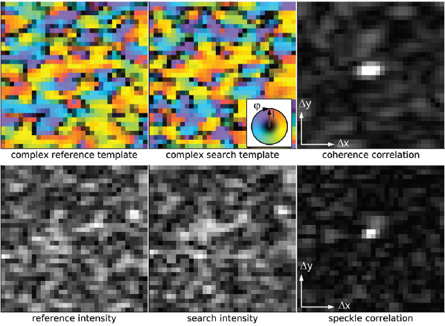
Figure 3.8. Top row: phase φ and intensity I (color; brightness) of reference and search template (32 × 32 pixels); right: the resulting coherence NCC. Bottom row: intensity of the same reference and search template; right: the resulting speckle NCC. For a color version of this figure, see www.iste.co.uk/cavalie/images.zip
3.2.2.2. Speckle tracking
For speckle tracking, the radar amplitude A or intensity I is used for equation [3.5]. Speckle tracking is successful when the speckle pattern is at least partially preserved between an image pair. Speckle tracking was suggested by Gray et al. (1998), who used the cross-correlation of detected radar images (intensity) to derive glacier velocity maps with both the range and azimuth direction. Similar to coherence tracking, speckle tracking allows for a very high spatial resolution in the offset field. For correlated speckle patterns, the speckle can be considered as correlated high-frequency noise, which generates a very sharp and narrow peak in the speckle cross-correlation function (Figure 3.8). A good description of speckle tracking combined with coherence tracking is given by Joughin (2002). Compared to coherence tracking, a slightly sharper peak can be obtained, as the intensity I = |A|2 doubles spatial frequencies in the image (see section 3.1.3 and Figure 3.8).
3.2.2.3. Intensity tracking
When the speckle pattern is completely uncorrelated, only larger features extending over multiple intensity pixels can be used for cross-correlation (Figure 3.9). In this case, the speckle pattern can be considered as uncorrelated (or incoherent) noise. To distinguish between intensity tracking of speckle and intensity tracking of image features containing uncorrelated speckle, the latter is also called incoherent intensity tracking, whereas speckle tracking can be considered as coherent intensity tracking.
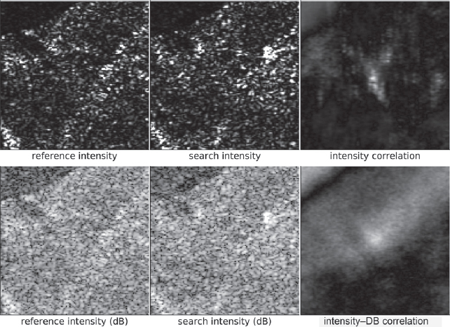
Figure 3.9. Top row: linearly scaled radar intensity of reference and search area (128 × 128 pixels) and the resulting incoherent intensity cross-correlation. Bottom row: intensity scaled in dB (same reference and search area as above) and the resulting intensity cross-correlation
To average out the incoherent speckle noise in the cross-correlation, considerably larger templates are required for intensity tracking. Typical template sizes vary between 64 × 64 and 256 × 256 pixels (Strozzi et al. 2002; Werner et al. 2005; Paul et al. 2015). Incoherent intensity tracking can be compared to offset tracking in optical imagery, as in both cases physical features are tracked. However, in optical imagery, speckle are absent and much smaller template sizes (e.g. 16×16 or 32×32 pixels) can be used.
As mainly large-scale features contribute to intensity tracking, the correlation function shows a much broader peak (Figure 3.9). As larger templates are required, computation of the cross-correlation can become computationally expensive. In the early days of computers, Vesecky et al. (1988) applied a pyramidal approach for calculating the correlation field to estimate the motion of sea ice. Today, with the availability of the fast Fourier transform (FFT), calculation of the cross-correlation can be sped up significantly when calculated in the frequency domain (see section 3.2.1.3).
When considering that speckle represents multiplicative noise for incoherent intensity tracking, it can be of advantage to convert the intensity into dB before cross-correlation. Thus, speckle can be considered as additive noise that reduces outliers and makes the correlation more robust (lower row in Figure 3.9).
3.2.2.4. Filters for image pre- and post-processing
To better extract the relevant feature patterns from the input images, various filters can be applied to the images before the cross-correlation. Spatial high-pass filters were shown to be effective in improving the coverage of successful tracking and the SNR of the cross-correlation (equation [3.6]) by de Lange et al. (2007).
The “phase correlation” method can be considered as a special case of a (high-pass) frequency filter, in which the frequency spectrum of the input data is completely flattened (normalized). Due to the flattened spectrum, only the phase terms eiφ of each frequency component are correlated, and hence this method is called “phase correlation” even though only real-valued intensity data are used as input. The normalization reduces the influence of long-wavelength structures and emphasizes high-frequency components in the image. For large enough templates and low enough noise, an extremely sharp correlation peak can be obtained (Schaum and McHugh 1991; Michel et al. 1999; Stone et al. 2001; Foroosh et al. 2002; Zitová and Flusser 2003). Nevertheless, emphasizing high-frequency image components makes the phase correlation method especially sensitive to speckle noise. A similar variant is “orientation correlation” where the orientation of intensity gradients is used as input for cross-correlation (Fitch et al. 2002). This method is often preferred for optical images with low noise, as it is less sensitive to illumination changes and shadow (Heid and Kääb 2012; Dehecq et al. 2015). However, due to its high-pass character, it is only of limited advantage for SAR images due to speckle.
Feature-based filters provide another method for pre-processing of SAR imagery. For example, stable point-like targets on mountain slopes can be discriminated from temporally variable speckle and their displacement can be tracked (Hu et al. 2013; Li et al. 2019). Edge-detection methods have been applied on sea ice followed by phase correlation on the speckle-free product (Karvonen et al. 2012).
Finally, before tracking results are used as input for geophysical models, post-processing can constrain the tracking results to the most probable or the most physical solution. An overview focused on glaciers is given in Chapter 11, sections 11.3.4 and 11.3.5.
3.2.3. SAR offset tracking using image series
With the increasing availability of SAR image series, offset tracking can be performed using many image pairs of the same area (data stack). The information contained in image series provides multiple independent measurements, which can make offset tracking more robust and/or precise. To exploit image series for offset tracking, stacking methods can be used by creating a data cube in which the stacked images represent the same area on the ground but are acquired under different conditions (e.g. different acquisition times). The image stack can be further processed to obtain a stack of cross-correlations or offset fields. Stacking methods have been suggested in various fields; for example, Meinhart et al. (2000) suggest them to improve tracking in particle image velocimetry (PIV) using image series. They subdivide the tracking process into three steps: image acquisition, cross-correlation and peak detection. In each of the three steps, stack-averaging can be applied for: 1) image acquisition by averaging each set of two image stacks before cross-correlation of the averaged stacks; 2) image correlation by averaging the stack of cross-correlations of consecutive image pairs before peak detection; and 3) peak detection by averaging the stack of offset vectors obtained from a series of cross-correlations. Each of the three variants has different advantages and disadvantages: for imagery with a low particle density (PIV), the density of the trackable particles is increased by image-averaging; satellite imagery, however, containing dense image content generally suffers from motion blur in the case of steadily moving features, but for features that can be considered stable during the averaging period, image noise can be reduced. Cross-correlation averaging can improve the signal-to-noise ratio, but for variable displacements, the correlation peak becomes blurred. Furthermore, only a single displacement estimate is undertaken after correlation averaging, whereas the averaging of offset vectors provides better statistics on the displacement dynamics and the estimation accuracy. The following two sections describe how to adapt the first two methods of cross-correlation averaging and image averaging to improve SAR offset tracking. Variants of the third method for post-processing of offset fields are probably most widely used and are described in Chapter 11, section 11.3.5.
3.2.3.1. Cross-correlation stacking
For a pair of non-identical image templates, their cross-correlation (or NCC) can be regarded as a noisy measurement of the offset between them. To enhance tracking, multiple NCCs can be stacked and averaged to reduce the noise and to improve the measurement accuracy. This principle, called the “average correlation method” by Meinhart et al. (2000), has been applied to estimate the velocity of quickly decorrelating ice falls using optical imagery, where it is referred to as “ensemble matching” (Altena and Kääb 2020). Similarly, Li et al. (2021) used this principle to estimate the velocity of alpine glaciers from SAR imagery strongly affected by speckle (incoherent intensity correlation, see section 3.2.2.3).
Let us assume that image templates are composed of a signal ![]() and noise
and noise ![]() as
as ![]() with ˆ indicating the Fourier transform. The NCC in the frequency domain [3.7] can be decomposed as:
with ˆ indicating the Fourier transform. The NCC in the frequency domain [3.7] can be decomposed as:
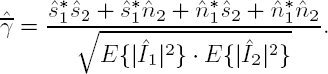

Figure 3.10. Top row: Great Aletsch Glacier intensity image (left) and velocity images obtained from pairwise NCC (middle) and by stacking seven NCC pairs of TerraSAR-X imagery and templates of 48 × 48 pixels (©DLR 2021). Bottom row: Sentinel-1A image (left) and velocity images obtained from pairwise NCC (middle) and by stacking 11 NCCs (right) using templates of 96 × 96 pixels (©ESA 2021). For a color version of this figure, see www.iste.co.uk/cavalie/images.zip
Here, the signal ![]() is assumed to contain all the correlated content that contributes to the correct template matching, and the noise
is assumed to contain all the correlated content that contributes to the correct template matching, and the noise ![]() to represent all the uncorrelated content. In equation [3.8], the shifted auto-correlation
to represent all the uncorrelated content. In equation [3.8], the shifted auto-correlation ![]() generates the signal to track, and the remaining components
generates the signal to track, and the remaining components ![]() add noise to the NCC and thus bring uncertainty to the measurement. In order to attain reliable offset estimates, a high SNR for the NCC must be achieved, and thus the term
add noise to the NCC and thus bring uncertainty to the measurement. In order to attain reliable offset estimates, a high SNR for the NCC must be achieved, and thus the term ![]() must generate a dominant peak that greatly surpasses the noise.
must generate a dominant peak that greatly surpasses the noise.
For NCC stacking, a time series of N coregistered images is collected with a revisit time of Δt, and an NCC is calculated from each pair of image templates with a temporal spacing of T = aΔt (a = 1, 2, 3... indicating integer multiples of the revisit time Δt). This results in a stack of N − a consecutive NCCs, in which each NCC captures a snapshot of the shift between the template pair. Assuming that image features move with constant velocities during acquisition of the image series, all NCCs in the stack represent identical offsets. Hence, the peaks of ![]() in all the NCCs should be located at the same position, whereas the noise term
in all the NCCs should be located at the same position, whereas the noise term ![]() remains independent and can be reduced by averaging the NCC stack. The principle of NCC stacking can be generalized to multiple image time series, such as image series acquired in different years, with different spectral or polarimetric channels or even from different sensors (e.g. optical and SAR). NCC stacking is relatively simple to implement but is currently limited to NCC pairs of identical temporal spacing T .
remains independent and can be reduced by averaging the NCC stack. The principle of NCC stacking can be generalized to multiple image time series, such as image series acquired in different years, with different spectral or polarimetric channels or even from different sensors (e.g. optical and SAR). NCC stacking is relatively simple to implement but is currently limited to NCC pairs of identical temporal spacing T .
Figure 3.10 shows that NCC stacking can effectively increase the spatial coverage of reliable velocity estimates for SAR offset tracking. In addition, Li et al. (2021) showed that NCC stacking produces reliable results already for a template size half as large as required for pairwise NCC. They also achieved a good performance gain for small stack sizes and thus the compromise on temporal resolution is limited.

Figure 3.11. (a) The temporal average of 10 SAR images (TerraSAR-X, ©DLR 2021) shows strong motion blur in the moving glacier. (b) After correcting for motion blur, the averaged images reveal many details of the glacier. (c) Velocity from intensity tracking of a single image pair (template size: 96 × 96 pixels, spacing: 32 pixels). (d) Velocity from autofocusing motion blur in a stack of 10 images (template size: 30 × 30 pixels). For a color version of this figure, see www.iste.co.uk/cavalie/images.zip
3.2.3.2. Autofocusing motion blur in image stacks
Temporal multi-looking causes strong motion blur on moving surfaces [Figure 3.11a], which is why the averaging of image stacks before cross-correlation, studied by Meinhart et al. (2000) for PIV with optical imagery of low particle density, cannot be directly applied to SAR images. Instead, Leinss et al. (2021b) used an autofocus method to combine offset estimation with temporal multi-looking through stack averaging. With the aim of generating two locally coinciding image templates, they split a stack of N images into two sub-stacks each containing N1 ≈ N2 ≈ N/2 images. Then, they sampled different velocities by correcting for the time- and velocity-dependent displacement in every image. When the correct local velocity was sampled, temporal multi-looking of the sub-stacks created two speckle-reduced and motion-compensated SAR images revealing fine details that spatially coincided and generated a high cross-correlation score. For sampled velocities that did not match the true velocity, details in the averaged sub-stacks became blurred, resulting in a lower cross-correlation score. The method outperforms pairwise incoherent intensity tracking because the multi-looking process strongly reduces temporally uncorrelated speckle in SAR images.
The method requires a stack of N radar intensity images Ii, acquired at times t1, ..., tN, during which most surface features remain visible. The images must be coregistered with sub-pixel precision on stable terrain or the orbit accuracy must be precise enough to ensure sub-pixel registration. Varying time intervals Δt between acquisitions and minor gaps in the time series pose no problem.
To avoid motion blur in the time-averaged sub-stacks, the shift of surface features must be corrected with precisely known offset fields. In contrast, we can determine the offset field by trying to obtain a temporally multi-looked SAR image where motion blur is minimized. To achieve this, the (so far unknown) time-dependent offset field (δx, δy)(x, y, t) can be approximated by the stationary velocity model
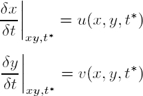
where u, v describe the two components of the local velocity vector, ![]() is approximately the mean acquisition time of the stack and δt = t − t∗ is the time interval during which the offset (δx, δy) occurs. Then, possible velocity values are sampled from a predefined distribution, for example a uniform distribution within a certain velocity range. The sampled velocity is used to estimate the time-dependent position (x′ , y′ )(δt) of features located at (x, y) at time t∗. For the i-th image in the stack, the position at time δti = ti − t∗ follows from the warping equations
is approximately the mean acquisition time of the stack and δt = t − t∗ is the time interval during which the offset (δx, δy) occurs. Then, possible velocity values are sampled from a predefined distribution, for example a uniform distribution within a certain velocity range. The sampled velocity is used to estimate the time-dependent position (x′ , y′ )(δt) of features located at (x, y) at time t∗. For the i-th image in the stack, the position at time δti = ti − t∗ follows from the warping equations
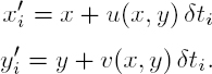
For a spatially constant velocity field, the warping equations describe a simple shear of the two image stacks. For an arbitrary but stationary velocity field, we can track image features that deviate for large δt from a linear trajectory using finite-step time integration of equation [3.10]. Using the warping equations for time-dependent interpolation of the original stacks, the offset-corrected image stacks can be obtained. Averaging each corrected sub-stack results in two offset-corrected temporally multi-looked intensity images in which speckle is strongly reduced.
To estimate the surface velocity field (u, v), the motion blur of the temporally multi-looked sub-stacks is iteratively evaluated for each sampled velocity until the blur is minimized. The motion blur in each iteration is quantified using a method adapted from the “passive phase detection autofocus” method of photographic cameras: two bundles of light rays, each entering the camera at opposite sides of the lens, generate two sub-images, and the focal-length is determined from the offset between the sub-image pair via cross-correlation. Similarly, we calculate the correlation score between the images ![]() obtained by averaging the offset-corrected sub-stack:
obtained by averaging the offset-corrected sub-stack:
i=k0
with (k0, kN) = (1, N1) for k = 1, (k0, kN) = (N1 + 1, N) for k = 2 and Nk = kN − k0 + 1. Already, with small Nk and a correctly chosen velocity, the images ![]() reveal surface structures that are hidden by speckle in single SAR images because the standard deviation of the intensity scales down with
reveal surface structures that are hidden by speckle in single SAR images because the standard deviation of the intensity scales down with ![]() (section 3.1.2). Due to reduced speckle, a relatively small template size can be used for the NCC. To compress the dynamic range and focus on small-scale features,
(section 3.1.2). Due to reduced speckle, a relatively small template size can be used for the NCC. To compress the dynamic range and focus on small-scale features, ![]() should be converted to dB and a high-pass filter can be applied before calculating the NCC.
should be converted to dB and a high-pass filter can be applied before calculating the NCC.
Each sampled velocity (u, v) shifts the images in the sub-stacks according to equation [3.10] and generates ![]() to calculate an NCC value
to calculate an NCC value ![]() The NCC score is maximized when the sampled velocity eliminates the motion blur of features in the stack, and more importantly, when the features revealed in
The NCC score is maximized when the sampled velocity eliminates the motion blur of features in the stack, and more importantly, when the features revealed in ![]() coincide. In practice, the sample velocity is applied to shift the entire image and the velocity that improves the local NCC score is stored. With sufficiently dense sampling, the optimal velocity for every image pixel can be found, which represents the estimated velocity field.
coincide. In practice, the sample velocity is applied to shift the entire image and the velocity that improves the local NCC score is stored. With sufficiently dense sampling, the optimal velocity for every image pixel can be found, which represents the estimated velocity field.
The velocity field can be iteratively refined, and thus the method is suitable to effectively track shear movements. The method requires that temporal variations in the velocity field be small, whereas there is no restriction on the spatial complexity of the observed flow patterns. In general, the uniform sampling of the velocity is computationally expensive as each iteration requires an interpolation of the entire image stack, the sum of the sub-stacks and the calculation of the NCC score. For effective velocity sampling, a pyramidal approach, as described by Vesecky et al. (1988), can be used.
As the method effectively correlates full-resolution speckle-reduced SAR imagery, the spatial resolution and also the coverage of the obtained velocity are significantly better compared to pairwise intensity cross-correlation, for which larger templates are required (compare Figure 3.11(c) vs. (d)). Compared to cross-correlation stacking, the method performs slightly better in robustness and accuracy. The reason is that in fact each image from one sub-stack is correlated with every image in the other sub-stack, resulting in (N/2)2 cross-correlations. In contrast, for cross-correlation stacking, only a consecutive series of N − 1 cross-correlations are evaluated. As a side product, the methods generate temporally multi-looked radar images that are free of motion blur (Figure 3.11(b)) and that can even be smoothly animated by an arbitrary choice of t∗ and a running average over a large image series (Leinss et al. 2021a).
3.2.4. Tracking from single and multiple orbits
Most imaging methods project information from a 3D terrain into two image dimensions. SAR sensors project the scene content, and hence also the true 3D displacement, into the slant-range and azimuth geometry. Single-pass interferometric SAR systems are an example where displacements perpendicular to the slant range and azimuth can be observed, as in, for example, Leinss and Bernhard (2021). In this section, we discuss projections of displacements into the desired geometry and considerations relevant for the radar imaging geometry.
3.2.4.1. Single-orbit tracking in slant-range coordinates
The projection of the 3D terrain into the SAR imaging geometry depends on the terrain and on the incidence angle (see Figure 3.3). As long as the incidence angle is constant between two acquisitions, offset tracking reveals only slant-range and azimuth displacement. However, small deviations from the reference orbit cause terrain-dependent distortions in the image content, resulting in terrain-dependent offset fields. To avoid such terrain-dependent offsets, the satellite orbit must be exactly repeated for every acquisition. As this is not always feasible, such geometric distortion can be corrected by DEM-based coregistration (Sansosti et al. 2006; Nitti et al. 2010). However, for SAR offset tracking, we should at least use imagery from the same orbit, as image features show different backscatter characteristics at different incidence angles. Speckle and coherence tracking are most sensitive to small deviations, as speckle can already decorrelate strongly for deviations of a few hundreds of meters from the reference orbit (see also the critical baseline described in Chapter 4, section 4.2.2).
Offset tracking in the native slant-range/azimuth geometry has the advantage that no resampling for orthorectification is required, providing slightly better image quality. Another interpolation can be avoided when tracking is done without resampling for coregistration and instead the offset field is corrected for global and terrain-induced shifts through post-processing. In the latter case, however, cross-correlation stacking and autofocusing motion blur (see sections 3.2.3.1 and 3.2.3.2) require geometry-dependent corrections.
To obtain displacements in a map geometry, the 2D projection of the displacement can be orthorectified (see also Chapter 11, section 11.3.3.3). However, it is crucial to specify that slant-range (line-of-slight) and azimuth displacements are shown or that additional, possibly model-based, transformation into other displacement geometries is applied.
3.2.4.2. Tracking in map coordinates
Offset tracking can also be applied to orthorectified radar images to obtain results directly in map coordinates. The oblique imaging geometry makes a precise orthorectification crucial to avoid image artifacts. For precise orthorectification, a SAR image simulated from an external DEM (Small et al. 1998; Small 2011) can be used as a reference to align the reference SAR image with the DEM used for orthorectification (Wegmüller 1999). DEM-based coregistration of a SAR image stack to a common reference scene is an advantage, in addition to coregistration of the reference scene to the simulated reference.
Working in map coordinates can simplify offset tracking because of the horizontally constant pixel spacing. However, tracking in map coordinates implies the implicit assumption of displacements parallel to the DEM slope. First, this is because the 3D displacement is projected to the slant range and azimuth, and then the orthorectification transforms the apparent slant-range displacement through the DEM-based orthorectification lookup-table into a horizontal displacement. While for slope-parallel displacements only the horizontal component is measured, non-slope-parallel displacements can introduce large biases into the obtained velocity maps.
Despite a constant pixel spacing in the orthorectified imagery, the slope-dependent effective resolution can vary strongly over the scene, which makes the tracking precision dependent on the terrain slope (see Figure 3.3). Another problem relates to small-scale features in the orthorectification DEM, which can distort or wrinkle the orthorectified images when the features move in time (e.g. moving glacier crevasses, growing forest).
3.2.4.3. Three-dimensional inversion
Three-dimensional displacement estimation (including east, north and up components) is an important subject in SAR displacement measurement exploration in relation to both offset tracking and SAR interferometry (Wright et al. 2004; Pathier et al. 2006). Displacement maps showing only line-of-slight and possibly also only azimuth displacements can make the comparison with other sources of information difficult. Furthermore, interpretation can be difficult for those not familiar with SAR geometries. The common approach is thus to estimate the 3D displacement, referred to as the common terrestrial coordinate, from InSAR or offset-tracking displacement measurements obtained from different directions (i.e. range and azimuth directions, different incidence angles, different orbit directions).

Figure 3.12. Geometric model of 3D displacement and the displacement in the range and azimuth directions
The problem can be resolved using a linear geometric model (Wright et al. 2004), as shown in Figure 3.12, and mathematically expressed as
where ![]() denotes the vector of N displacement measurements in different directions (LOS, azimuth) obtained from offset tracking or InSAR, and u is the vector containing the true 3D displacement components to estimate. The matrix P is the N × 3 projection matrix, where the rows define the projection either into the slant-range (pLOS,i) or azimuth direction (paz,i). The projections depend on the incidence angle θi and the azimuth heading angle φi of each acquisition geometry used. φi is defined as between the direction of the satellite trajectory and north. The projections are given by the unit row vectors
denotes the vector of N displacement measurements in different directions (LOS, azimuth) obtained from offset tracking or InSAR, and u is the vector containing the true 3D displacement components to estimate. The matrix P is the N × 3 projection matrix, where the rows define the projection either into the slant-range (pLOS,i) or azimuth direction (paz,i). The projections depend on the incidence angle θi and the azimuth heading angle φi of each acquisition geometry used. φi is defined as between the direction of the satellite trajectory and north. The projections are given by the unit row vectors

To solve equation [3.12], the least-squares approach is commonly used:
with Σr being the error covariance of displacement measurements in r. Its main role consists of appropriately weighting displacement measurements of different uncertainties and propagating the uncertainty from r to u. In many cases, a diagonal matrix is used for the sake of simplicity, assuming independence of each displacement measurement. In the case of measurements sharing the same reference/secondary images, the latter assumption may not hold and improved estimations of the covariance matrix Σr may be necessary (Teunissen and Amiri-Simkooei 2008). Σr can also be approximated by other quality indicator parameters, such as interferometric coherence or cross-correlation coefficients.
Since u is a vector with three components, there should be displacement measurements in at least three directions in r. Tracking results from descending and ascending passes are therefore often combined. However, outside of high latitudes, the azimuth directions of the ascending and descending passes are nearly collinear. In practice, they are often considered as the same contribution to the least-square solution.
Through equation [3.14], a large number of displacement measurements can be transformed into a single 3D displacement result. Besides the ease of interpretation and comparison, another main feature of interest lies in the reduction of the uncertainty. The uncertainty of the 3D displacement obtained is smaller than that of any displacement measurement in r. For a random uncertainty, the uncertainty decreases with the number of displacement measurements used. Therefore, the use of all available displacement measurements is preferred, knowing that the eventual interdependence between different measurements can result in an underestimation of the uncertainty of the 3D displacement. However, when systematic uncertainty (e.g. from orbit uncertainties) is present, fuzzy logic allows us to better describe the uncertainty due to data fusion and provides an upper bound for the uncertainty (Yan et al. 2012). The extraction of 3D displacement fields also simplifies the comparison of results between different sensors, models and field measurements (Yan et al. 2013).
3.2.5. Summary
This chapter provided a brief introduction to the SAR imaging method, the imaging geometry and the origin of radar speckle. The basic principles of offset tracking using the cross-correlation of pairs of image templates were introduced, followed by details of how to characterize the correlation score and the signal-to-noise ratio and how to efficiently calculate the normalized cross-correlation in the frequency domain. Depending on the temporal coherence of the speckle pattern in SAR imagery, different methods, such as coherence tracking, speckle tracking or intensity tracking, can be applied, with the latter requiring significantly larger image templates due to uncorrelated speckle noise. To make tracking more robust, stacks of cross-correlation functions or motion-compensated image stacks can be evaluated. We concluded this chapter by outlining the advantages and disadvantages of offset tracking using SAR imagery radar and map coordinates and describing a common method to combine offset estimates from multiple orbits and obtain 3D displacements.
3.3. Acknowledgments
The authors thank Anna Wendleder and Tazio Strozzi for their careful reviews and comments that helped to improve this chapter.
3.4. References
Altena, B. and Kääb, A. (2020). Ensemble matching of repeat satellite images applied to measure fast-changing ice flow, verified with mountain climber trajectories on Khumbu icefall, Mount Everest. Journal of Glaciology, 66(260), 905–915.
Balci, M. and Foroosh, H. (2006). Subpixel estimation of shifts directly in the Fourier domain. IEEE Transactions on Image Processing, 15(7), 1965–1972.
Bindschadler, R.A. and Scambos, T.A. (1991). Satellite-image-derived velocity field of an Antarctic ice stream. Science, 252(5003), 242–246.
Chen, J. and Katz, J. (2005). Elimination of peak-locking error in PIV analysis using the correlation mapping method. Measurement Science and Technology, 16(8), 1605–1618.
De Zan, F. (2014). Accuracy of incoherent speckle tracking for circular Gaussian signals. IEEE Geoscience and Remote Sensing Letters, 11(1), 264–267.
Debella-Gilo, M. and Kääb, A. (2011). Sub-pixel precision image matching for measuring surface displacements on mass movements using normalized cross-correlation. Remote Sensing of Environment, 115(1), 130–142.
Dehecq, A., Gourmelen, N., Trouvé, E. (2015). Deriving large-scale glacier velocities from a complete satellite archive: Application to the Pamir–Karakoram–Himalaya. Remote Sensing of Environment, 162, 55–66.
Derauw, D. (1999). DInSAR and coherence tracking applied to glaciology: The example of Shirase Glacier. Proceedings of the FRINGE, ESA.
Fitch, A.J., Kadyrov, A., Christmas, W.J., Kittler, J. (2002). Orientation correlation. Proceedings of 13th British Machine Vision Conference, 1–10.
Foroosh, H., Zerubia, J.B., Berthod, M. (2002). Extension of phase correlation to subpixel registration. IEEE Transactions on Image Processing, 11(3), 188–200.
Funning, G.J., Parsons, B., Wright, T.J., Jackson, J.A., Fielding, E.J. (2005). Surface displacements and source parameters of the 2003 Bam (Iran) earthquake from Envisat advanced synthetic aperture radar imagery. Journal of Geophysical Research: Solid Earth, 110(B9).
Gray, A.L., Mattar, K.E., Vachon, P.W., Bindschadler, R., Jezek, K.C., Forster, R., Crawford, J.P. (1998). InSAR results from the RADARSAT Antarctic mapping mission data: Estimation of glacier motion using a simple registration procedure. IEEE International Geoscience and Remote Sensing Symposium, 3, 1638–1640.
Heid, T. and Kääb, A. (2012). Evaluation of existing image matching methods for deriving glacier surface displacements globally from optical satellite imagery. Remote Sensing of Environment, 118, 339–355.
Hoge, W. (2003). A subspace identification extension to the phase correlation method. IEEE Transactions on Medical Imaging, 22(2), 277–280.
Hu, X., Wang, T., Liao, M. (2013). Measuring coseismic displacements with point-like targets offset tracking. IEEE Geoscience and Remote Sensing Letters, 11(1), 283–287.
Joughin, I. (2002). Ice-sheet velocity mapping: A combined interferometric and speckle-tracking approach. Annals of Glaciology, 34, 195–201.
Karvonen, J., Cheng, B., Vihma, T., Arkett, M., Carrieres, T. (2012). A method for sea ice thickness and concentration analysis based on SAR data and a thermodynamic model. The Cryosphere, 6(6), 1507–1526.
de Lange, R., Luckman, A., Murray, T. (2007). Improvement of satellite radar feature tracking for ice velocity derivation by spatial frequency filtering. IEEE Transactions on Geoscience and Remote Sensing, 45(7), 2309–2318.
Leinss, S. and Bernhard, P. (2021). TanDEM-X: Deriving InSAR height changes and velocity dynamics of Great Aletsch Glacier. IEEE Journal of Selected Topics in Applied Earth Observervation and Remote Sensing, 14, 1–18.
Leinss, S., Li, S., Frey, O. (2021a). Flow animation of Great Aletsch Glacier generated by autofocusing temporally multilooked SAR time series. Video, ETH Research Collection.
Leinss, S., Li, S., Frey, O. (2021b). Measuring glacier velocity by autofocusing temporally multilooked SAR time series. IEEE International Geoscience and Remote Sensing Symposium, 5493–5496.
Leprince, S., Barbot, S., Ayoub, F., Avouac, J.-P. (2007). Automatic and precise orthorectification, coregistration, and subpixel correlation of satellite images, application to ground deformation measurements. IEEE Transactions on Geoscience and Remote Sensing, 45(6), 1529–1558.
Li, M., Zhang, L., Shi, X., Liao, M., Yang, M. (2019). Monitoring active motion of the Guobu landslide near the Laxiwa hydropower station in China by time-series point-like targets offset tracking. Remote Sensing of Environment, 221, 80–93.
Li, S., Leinss, S., Hajnsek, I. (2021). Cross-correlation stacking for robust offset tracking using SAR image time-series. IEEE Journal of Selected Topics in Applied Earth Observations and Remote Sensing, 14, 4765–4778.
Lucchitta, B.K. and Ferguson, H.M. (1986). Antarctica: Measuring glacier velocity from satellite images. Science, 234(4780), 1105–1108.
Meinhart, C.D., Wereley, S.T., Santiago, J.G. (2000). A PIV algorithm for estimating time-averaged velocity fields. Journal of Fluids Engineering, 122(2), 285–289.
Michel, R., Avouac, J.-P., Taboury, J. (1999). Measuring ground displacements from SAR amplitude images: Application to the Landers earthquake. Geophysical Research Letters, 26(7), 875–878.
Nitti, D.O., Hanssen, R.F., Refice, A., Bovenga, F., Nutricato, R. (2010). Impact of DEM-assisted coregistration on high-resolution SAR interferometry. IEEE Transactions on Geoscience and Remote Sensing, 49(3), 1127–1143.
Oliver, C. and Quegan, S. (2004). Understanding Synthetic Aperture Radar Images. SciTech Publishing, Raleigh.
Olmsted, C. (1993). Alaska SAR Facility – Scientific SAR User’s Guide. Document.
Pathier, E., Fielding, E.J., Wright, T.J., Walker, R., Parsons, B.E., Hensley, S. (2006). Displacement field and slip distribution of the 2005 Kashmir earthquake from SAR imagery. Geophysical Research Letters, 33(20).
Paul, F., Bolch, T., Kääb, A., Nagler, T., Nuth, C., Scharrer, K., Shepherd, A., Strozzi, T., Ticconi, F., Bhambri, R., Berthier, E., Bevan, S., Gourmelen, N., Heid, T., Jeong, S., Kunz, M., Lauknes, T.R., Luckman, A., Merryman Boncori, J.P., Moholdt, G., Muir, A., Neelmeijer, J., Rankl, M., Van Looy, J., Van Niel, T. (2015). The glaciers climate change initiative: Methods for creating glacier area, elevation change and velocity products. Remote Sensing of Environment, 162, 408–426.
Rosen, P.A., Hensley, S., Joughin, I.R., Fuk, K.L., Madsen, S.N., Rodriguez, E., Goldstein, R.M. (2000). Synthetic aperture radar interferometry. Proceedings of the IEEE, 88(3), 333–382.
Sansosti, E., Berardino, P., Manunta, M., Serafino, F., Fornaro, G. (2006). Geometrical SAR image registration. IEEE Transactions on Geoscience and Remote Sensing, 44(10), 2861–2870.
Scambos, T.A., Dutkiewicz, M.J., Wilson, J.C., Bindschadler, R.A. (1992). Application of image cross-correlation to the measurement of glacier velocity using satellite image data. Remote Sensing of Environment, 42(3), 177–186.
Schaum, A. and McHugh, M. (1991). Analytic methods of image registration: Displacement estimation and resampling. Technical report, Naval Research Lab, Washington DC.
Small, D. (2011). Flattening gamma: Radiometric terrain correction for SAR imagery. IEEE Transactions on Geoscience and Remote Sensing, 49(8), 3081–3093.
Small, D., Holecz, F., Meier, E., Nuesch, D. (1998). Absolute radiometric correction in rugged terrain: A plea for integrated radar brightness. IEEE International Geoscience and Remote Sensing Symposium, 330–332.
Stone, H., Orchard, M., Chang, E.-C., Martucci, S. (2001). A fast direct Fourier-based algorithm for subpixel registration of images. IEEE Transactions on Geoscience and Remote Sensing, 39(10), 2235–2243.
Strozzi, T., Luckman, A., Murray, T., Wegmüller, U., Werner, C.L. (2002). Glacier motion estimation using SAR offset-tracking procedures. IEEE Transactions on Geoscience and Remote Sensing, 40(11), 2384–2391.
Teunissen, P.J. and Amiri-Simkooei, A. (2008). Least-squares variance component estimation. Journal of Geodesy, 82(2), 65–82.
Tong, X., Ye, Z., Xu, Y., Gao, S., Xie, H., Du, Q., Liu, S., Xu, X., Liu, S., Luan, K., Still, U. (2019). Image registration with Fourier-based image correlation: A comprehensive review of developments and applications. IEEE Journal of Selected Topics in Applied Earth Observations and Remote Sensing, 12(10), 4062–4081.
Trouvé, E., Nicolas, J.-M., Maitre, H. (1998). Improving phase unwrapping techniques by the use of local frequency estimates. IEEE Transactions on Geoscience and Remote Sensing, 36(6), 1963–1972.
Vesecky, J.F., Samadani, R., Smith, M.P., Daida, J.M., Bracewell, R.N. (1988). Observation of sea-ice dynamics using synthetic aperture radar images: Automated analysis. IEEE Transactions on Geoscience and Remote Sensing, 26(1), 38–48.
Wegmüller, U. (1999). Automated terrain corrected SAR geocoding. IEEE International Geoscience and Remote Sensing Symposium, 3, 1712–1714.
Werner, C., Wegmüller, U., Strozzi, T., Wiesmann, A. (2005). Precision estimation of local offsets between pairs of SAR SLCs and detected SAR images. IEEE International Geoscience and Remote Sensing Symposium, 7, 4803.
Wright, T.J., Parsons, B.E., Lu, Z. (2004). Toward mapping surface deformation in three dimensions using InSAR. Geophysical Research Letters, 31(1).
Yan, Y., Mauris, G., Trouvé, E., Pinel, V. (2012). Fuzzy uncertainty representations of co-seismic displacement measurements issued from SAR imagery. IEEE Transactions on Instrumentation and Measurement, 61(5), 1278–1286.
Yan, Y., Pinel, V., Trouvé, E., Pathier, E., Perrain, J., Bascou, P., Jouanne, F. (2013). Coseismic slip distribution of the 2005 Kashmir earthquake from SAR amplitude image correlation and differential interferometry. Geophysical Journal International, 193(1), 29–46.
Zitová, B. and Flusser, J. (2003). Image registration methods: A survey. Image and Vision Computing, 21, 977–1000.