
6
The Interferometric Phase: Unwrapping and Closure Phase
Béatrice PINEL-PUYSSÉGUR1 , Francesco DE ZAN2 and Johann CHAMPENOIS1
1CEA, DAM, DIF, Arpajon, France
2Remote Sensing Technology Institute, German Aerospace Center (DLR), Oberpfaffenhofen, Germany
6.1. Introduction
This chapter describes some properties of interferometric phase and the associated processing. Interferometric phase is naturally given as a wrapped number and needs to be unwrapped to obtain a valuable measurement. Besides its use in InSAR, phase unwrapping is a mathematical problem arising in several fields of optics, such as laser interferometry, sonar and nuclear magnetic resonance. In this chapter, only methods derived from the literature on InSAR are described. Historically, phase unwrapping algorithms were applied to single interferograms, as satellite acquisition rates were low. A fundamental property of the unwrapped phase in the spatial domain is that the closure of the phase around a spatial loop is null. This property, called irrotationality, is used by all unwrapping algorithms. The last 20 years have exhibited an unprecedented increase in the amount of data, which has led to the development of 3D phase unwrapping algorithms, the third dimension being time: instead of unwrapping each interferogram separately, the whole time series of interferograms is unwrapped at once. Naturally, the principles used in 2D algorithms were extended in 3D, especially irrotationality. However, in the last 10 years, several authors have noticed that the nullity of closure phase is only approximate in the time dimension when the interferograms are multi-looked1. This chapter first describes the unwrapping problem then phase closure in the time domain.
As seen in the preceeding chapters, the unwrapping process is a crucial and difficult step that has given rise to an abundant literature. Section 6.2 gives an non-extensive overview of the phase unwrapping algorithms used in InSAR. Some common prerequisites are given in section 6.2.1, followed by the description of several algorithms. Despite the diversity of the algorithms, phase unwrapping errors still occur. Thus, various algorithms have been developed to automatically correct such errors and several are described in section 6.2.6, with some of them based on the analysis of closure phase.
Section 6.3 describes the closure phase and its mathematical properties and provides examples of physical phenomena that can explain it, such as volumetric effects associated with significant normal baselines or changes in the dielectric constant of the radar targets. The section shows also how the presence of non-zero closure phases is linked to a risk of a bias in the retrieved deformation parameters, depending on the algorithm and configuration.
6.2. Phase unwrapping algorithms and limitation of phase unwrapping errors
6.2.1. The problem of phase unwrapping and some prerequisites
6.2.1.1. What is phase unwrapping?
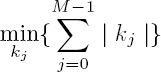
The phase of an interferogram is wrapped, i.e. its value is only known modulo 2π. The notations here follow those of Costantini (1998). Let Φ(i, j) be the unwrapped phase at indices (i, j), where i is the line index, i = 0, 1, ..., N −1 and j is the column index, j = 0, 1, ..., M −1. The rectangular definition domain of (i, j) is noted S. The wrapped interferogram phase is noted Ψ(i, j) and lies in the interval ![]() 2 The unwrapping process reconstructs Φ(i, j) from Ψ(i, j). Precisely, for each (i, j) ∈ S, as Ψ(i, j) is equal to Φ(i, j) modulo 2π, we have:
2 The unwrapping process reconstructs Φ(i, j) from Ψ(i, j). Precisely, for each (i, j) ∈ S, as Ψ(i, j) is equal to Φ(i, j) modulo 2π, we have:
Thus, the unwrapping process can be equivalently seen as reconstructing the k(i, j) from the Ψ(i, j), for (i, j) ∈ S. In the absence of any noise and if the phase gradient absolute value between any two neighboring pixels is less than π, then phase unwrapping is unambiguous. Problems arise if any of the two former conditions are not fulfilled, which is almost always the case in practice. In the following, some notions common to most algorithms as well as some notations are defined.
6.2.1.2. Wrapped and unwrapped phase gradients
In practice, most unwrapping algorithms first evaluate the wrapped phase gradients in the two directions (i.e. line and column) in order to estimate the unwrapped phase gradients. Once the phase gradients have been correctly estimated, the unwrapped phase is simply evaluated by integration. However, why begin with gradient estimation? In fact, the knowledge of Ψ required to reconstruct Φ without further assumptions is impossible: for each (i, j), any Φ(i, j) equal to Ψ(i, j) − 2πk(i, j) with k(i, j) ∈ Z would be possible, leading to an infinity of solutions for each pixel. However, if Φ is continuous almost everywhere, as it should be intuitively, then its gradient should be “small” with respect to 2π almost everywhere. This essential and heuristic assumption is the basis of most unwrapping algorithms. However, it also creates unwrapping errors wherever it does not apply.
Still following the notations of Costantini (1998), let us define the subsets of the definition domain where the gradient is defined: S1 = (i, j), i ∈ 0, 1, ..., N − 2, j ∈ 0, 1, ...M − 1 and S2 = (i, j), i ∈ 0, 1, ..., N − 1, j ∈ 0, 1, ...M − 2. The discrete partial derivatives in the line and column directions of a function F (i, j) defined on S are noted:
The gradient of Φ is a vector field:
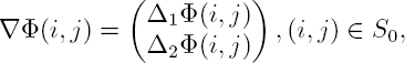
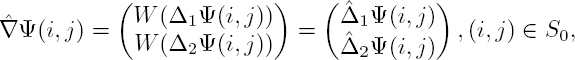
where S0 = S1 ∩ S2. Figure 6.1 illustrates the different notations. From the measurements Ψ, we aim to reconstruct ∇Φ. First, the gradient of Ψ is computed from equations [6.2] and [6.3]. Let us define the wrapping operator W such that3:
In order to fulfill the “smooth gradient” assumption, the gradient of Φ is heuristically estimated by the “wrapped-differences-of-wrapped-phases estimator”, as named by Bamler and Hartl (1998):
In practice, this last equation is the application of the “smooth gradient” assumption, as it constrains each component of ![]() to be smaller than π in absolute value. As
to be smaller than π in absolute value. As ![]() is an estimator of ∇Φ, this estimate will be correct as soon as both components of ∇Φ are smaller than π in absolute value, which is the case for most pixels in practice. However, whenever any of the components of ∇Φ is greater than π in absolute value,
is an estimator of ∇Φ, this estimate will be correct as soon as both components of ∇Φ are smaller than π in absolute value, which is the case for most pixels in practice. However, whenever any of the components of ∇Φ is greater than π in absolute value, ![]() underestimates the gradient in absolute value. This arises for noisy or aliased interferograms. As explained in the next section, the rotational is a tool used to detect such cases. Some authors have suggested robust approaches to estimate the fringe rate from noisy wrapped interferograms, which notably reduce the occurrence of such underestimation (Trouvé et al. 1998). Unfortunately, such methods are not systematically used.
underestimates the gradient in absolute value. This arises for noisy or aliased interferograms. As explained in the next section, the rotational is a tool used to detect such cases. Some authors have suggested robust approaches to estimate the fringe rate from noisy wrapped interferograms, which notably reduce the occurrence of such underestimation (Trouvé et al. 1998). Unfortunately, such methods are not systematically used.
6.2.1.3. Notions of the rotational, residue and congruency
The rotational (or curl) of the vector field ∇Φ can be expressed in its discrete version (e.g. Bamler and Hartl 1998):
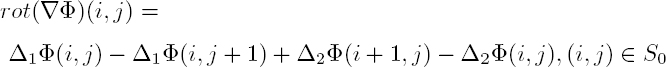
Figure 6.1a illustrates how the rotational is computed. Although the rotational is relative to the square delimited by indices (i, j), (i+1, j), (i+1, j+1) and (i, j+1), it is attributed to the lower-left index (i, j). Following many authors, fractions of phase cycles are represented in Figure 6.1b and c, i.e. phases are divided by 2π. Thus, if the phase lies in [−π, π[, the fraction of cycles lies in [−0.5, 0.5[. Figure 6.1b shows an example of unwrapped phase Φ, its gradient and its rotational. Due to the central pixel valuing 0.6, three gradients of Φ are greater than 0.5 in absolute value. However, the rotational of ![]() is 0 for every square, as these high gradients are correctly compensated for by the three other terms of the rotational. Figure 6.1c represents the wrapped phase Ψ, the gradient components of
is 0 for every square, as these high gradients are correctly compensated for by the three other terms of the rotational. Figure 6.1c represents the wrapped phase Ψ, the gradient components of ![]() and its rotational. Due to wrapping, the central value of Φ valuing 0.6 is replaced by -0.4 and the three highest gradients are underestimated. The rotational of
and its rotational. Due to wrapping, the central value of Φ valuing 0.6 is replaced by -0.4 and the three highest gradients are underestimated. The rotational of ![]() values +1 and -1 on the two right-side squares as they each contain one erroneous gradient component. These two erroneous rotational values are called residues. More generally, a residue is a pixel for which the rotational computed as in equation [6.7] is non-zero. Due to wrapping, the rotational of a residue values
values +1 and -1 on the two right-side squares as they each contain one erroneous gradient component. These two erroneous rotational values are called residues. More generally, a residue is a pixel for which the rotational computed as in equation [6.7] is non-zero. Due to wrapping, the rotational of a residue values ![]() 4. If k is positive (respectively, negative), the residue is called positive (respectively, negative). Let us note that on the left-side squares, there are two erroneous estimates of the gradient components with opposite sign so that the rotational of
4. If k is positive (respectively, negative), the residue is called positive (respectively, negative). Let us note that on the left-side squares, there are two erroneous estimates of the gradient components with opposite sign so that the rotational of ![]()
This toy example illustrates the fundamental problem of unwrapping. An unwrapped phase field Φ(i, j), (i, j) ∈ S exists if and only if (from equation 5 in Costantini (1998)) the gradients in the line and column directions fulfill the following condition:
This condition means that ∇Φ, which is defined on a discrete space, should be a conservative or irrotational vector field. If this condition holds, then it is possible to find a real-valued function Φ by integration, up to an additive constant (Costantini 1998), which will be independent of the integration path. Thus, the aim of several unwrapping algorithms is to estimate the gradient field ∇Φ such that condition [6.8] holds. In practice, only Ψ is known and ![]() may be non-conservative at some places. Some algorithms (minimum cost flow (MCF), branch cuts) identify where the rotational of
may be non-conservative at some places. Some algorithms (minimum cost flow (MCF), branch cuts) identify where the rotational of ![]() is non-zero, i.e. where
is non-zero, i.e. where ![]() does not correctly estimate ∇Φ.
does not correctly estimate ∇Φ.
Finally, for some unwrapping algorithms, the reconstructed field ![]() has the following property, called congruency:
has the following property, called congruency:
Although most algorithms estimate a congruent unwrapped phase, it will be seen that some others do not.
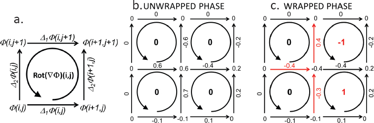
Figure 6.1. (a) Notations for the phase gradient (represented by the straight arrows) and the rotational (represented by the curly arrows). (b) Example of an unwrapped phase and associated gradient and rotational. (c) Same example as in b but after wrapping. Values where the phase gradient is greater than a 0.5 cycle in absolute value are wrapped (red arrows) and residues (–1 and +1) arise even if the rotational is zero for unwrapped phase. For a color version of this figure, see www.iste.co.uk/cavalie/images.zip
6.2.1.4. Other useful prerequisites
Different norms and pseudo-norms are used by unwrapping algorithms. The phase unwrapping problem is often stated as a minimization problem in order to evaluate the unknowns ![]() from the measurements
from the measurements ![]() Weights w1(i, j) and w2(i, j) are attributed to each pixel (i, j) depending on the confidence on the gradient measure in the two directions. If the minimization function F is assumed to be separable in each direction, then it can be written as (e.g. Chen and Zebker (2000)):
Weights w1(i, j) and w2(i, j) are attributed to each pixel (i, j) depending on the confidence on the gradient measure in the two directions. If the minimization function F is assumed to be separable in each direction, then it can be written as (e.g. Chen and Zebker (2000)):
The factor p determines the metric chosen to compare ![]() Depending on the author, F is minimized on Φ or on ∇Φ and p is set to 0, 1 or 2, leading, respectively, to minimization with an L0 pseudo-norm, L1 norm or L2 norm. The L0 pseudo-norm of a vector is simply the number of non-zero elements of this vector. Strictly speaking, it is not a norm because it is not homogeneous. However, it is used by several authors (e.g. Chen and Zebker 2000). The MCF algorithm uses the L1 norm (Costantini 1998), whereas the L2 norm is used by the least-squares unwrapping algorithm (Ghiglia and Romero 1994). Chen and Zebker (2000) show that the L0 pseudo-norm problem is NP-hard, which means that it cannot be solved exactly by any algorithm in a polynomial time (unless P and NP problem classes are equivalent). Thus, the approaches aiming to solve this problem are in fact heuristics to approximate the solution.
Depending on the author, F is minimized on Φ or on ∇Φ and p is set to 0, 1 or 2, leading, respectively, to minimization with an L0 pseudo-norm, L1 norm or L2 norm. The L0 pseudo-norm of a vector is simply the number of non-zero elements of this vector. Strictly speaking, it is not a norm because it is not homogeneous. However, it is used by several authors (e.g. Chen and Zebker 2000). The MCF algorithm uses the L1 norm (Costantini 1998), whereas the L2 norm is used by the least-squares unwrapping algorithm (Ghiglia and Romero 1994). Chen and Zebker (2000) show that the L0 pseudo-norm problem is NP-hard, which means that it cannot be solved exactly by any algorithm in a polynomial time (unless P and NP problem classes are equivalent). Thus, the approaches aiming to solve this problem are in fact heuristics to approximate the solution.
Finally, several authors use graph theory vocabulary. Indeed, a 2D interferogram can be viewed as a set of data points that form the nodes or vertices of a graph. When only a subset of pixels is selected (sparse data, for example, in the permanent scatterers technique), pixels are often linked by a Delaunay triangulation, forming the edges (or arcs) of the graph. In the temporal domain as well, the set of all acquisition dates can be viewed as a graph where each date is a node and each interferogram between two acquisitions is an edge. In a 3D domain (space and time), one pixel at a given date defines a node and the differential between two nodes (even if in different locations and different times) can be considered as an edge.
6.2.2. A short history of unwrapping methods in InSAR
One of the first unwrapping algorithms was the residue-cut tree algorithm (Goldstein et al. 1988), which identifies where the integration process is forbidden. As this algorithm is time-consuming, Ghiglia and Romero (1994) proposed a least-squares approach, which is very fast but has some drawbacks, as the unwrapped phase gradient is underestimated. Then, a family of algorithms using network-based approaches was developed, beginning with the minimum cost flow algorithm (Costantini 1998). Since the 2000s, data increases have lead to the generalization of 2D unwrapping techniques to 3D, the third dimension being time. Another novelty of this period is that the sampling of data may not be regular anymore, following the development of InSAR time-series processing on sparse data points, such as the persistent scatterers technique (Ferretti et al. 2001). Finally, the redundancy of the InSAR time series also allowed the development of algorithms correcting unwrapping errors during the unwrapping process or a posteriori. The different unwrapping algorithms can be classified in several ways. Here, they are divided into the three large families originally developed for 2D problems and presented in three sections: the residue cut-type methods, the least-squares approach and the network-based algorithms. For the first and last families, 3D methods are also described.
6.2.3. Residue-cut tree algorithm, variants and 3D generalization
The residue-cut tree algorithm (Goldstein et al. 1988) is a still very widely used algorithm, despite being one of the first described in the InSAR literature. The principle of this algorithm is to identify every residue on the image by computing the rotational of ![]() following equations [6.6] and [6.7]. Then, every point where the rotational is non-zero is called either a positive or negative residue. Goldstein et al. (1988) state that an integration path enclosing a single residue produces an inconsistency in the unwrapped phase, whereas an integration path enclosing as many positive as negative residues does not. Thus, cuts are placed between couples of positive and negative residues to forbid any integration path across these cuts. The unwrapped phase difference between two pixels on opposite sides of a cut exceeds one half-cycle. In order to minimize the total discontinuity of the unwrapped phase, the aim is to find the overall shortest set of cuts pairing a positive and a negative residue. When a residue is found, another residue is searched for in a 3x3 box centered on the first one. If the second residue has the opposite sign, then a cut is placed in between and marked as “uncharged”. Otherwise, the search begins again from the second residue. If no residue is found in the boxes, the size of the boxes is multiplied by 2. This algorithm works well in areas where residues are sparse but can create isolated regions in areas with a high density of residues. In such a case, only one isolated region can be unwrapped as there is no integration path between two regions that do not cross a cut. Thus, large parts on an interferogram may remain wrapped. Figure 6.2, adapted from Chen and Zebker (2000, 2001), shows an example of an interferogram affected by topographic fringes. This interferogram has been unwrapped by several unwrapping algorithms with adapted weights and the residual of the unwrapped interferogram with respect to a reference synthetic interferogram generated by an external DEM (see Chen and Zebker (2000) for details) is shown from b to g: the closer to zero the residual is, the better the unwrapping. The residual of the residue-cut tree algorithm solution is shown in Figure 6.2b. Although this algorithm performs well on the unwrapped area, a large area shown in black remains wrapped.
following equations [6.6] and [6.7]. Then, every point where the rotational is non-zero is called either a positive or negative residue. Goldstein et al. (1988) state that an integration path enclosing a single residue produces an inconsistency in the unwrapped phase, whereas an integration path enclosing as many positive as negative residues does not. Thus, cuts are placed between couples of positive and negative residues to forbid any integration path across these cuts. The unwrapped phase difference between two pixels on opposite sides of a cut exceeds one half-cycle. In order to minimize the total discontinuity of the unwrapped phase, the aim is to find the overall shortest set of cuts pairing a positive and a negative residue. When a residue is found, another residue is searched for in a 3x3 box centered on the first one. If the second residue has the opposite sign, then a cut is placed in between and marked as “uncharged”. Otherwise, the search begins again from the second residue. If no residue is found in the boxes, the size of the boxes is multiplied by 2. This algorithm works well in areas where residues are sparse but can create isolated regions in areas with a high density of residues. In such a case, only one isolated region can be unwrapped as there is no integration path between two regions that do not cross a cut. Thus, large parts on an interferogram may remain wrapped. Figure 6.2, adapted from Chen and Zebker (2000, 2001), shows an example of an interferogram affected by topographic fringes. This interferogram has been unwrapped by several unwrapping algorithms with adapted weights and the residual of the unwrapped interferogram with respect to a reference synthetic interferogram generated by an external DEM (see Chen and Zebker (2000) for details) is shown from b to g: the closer to zero the residual is, the better the unwrapping. The residual of the residue-cut tree algorithm solution is shown in Figure 6.2b. Although this algorithm performs well on the unwrapped area, a large area shown in black remains wrapped.
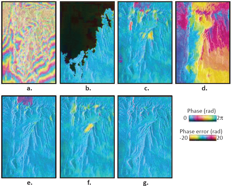
Figure 6.2. (a) Interferogram affected by topography. (b–g) Residuals of interferograms unwrapped by different methods with respect to a reference synthetic interferogram: (b) residue-cut tree (c) minimum-spanning tree; (d) least squares; (e) minimum cost flow; (f) dynamic cost canceling; (g) the statistical-cost network-flow algorithm for phase unwrapping (SNAPHU). This figure is adapted with permission from the Journal of the Optical Society of America (JOSA). For a color version of this figure, see www.iste.co.uk/cavalie/images.zip
Chen and Zebker (2000) enhanced the residue-cut tree algorithm to solve the problem of disconnected regions. This problem arises from the strategy of iteratively linking residues in the neighborhood of the current residue, which can lead to closed branch cuts for a high residue density. Instead, they proposed a minimum-spanning tree algorithm. As in the residue-cut approach, the tree forbids integration paths. The advantage of this approach is that, by definition, a tree never contains any branch closed on itself. Although performing well for the example shown and effectively unwrapping the whole interferogram (see Figure 6.2c), the authors mention that this approach suffers from a lack of accuracy when residue density is high.
Hooper and Zebker (2007) proposed two algorithms for 3D phase unwrapping. We focus here on the first algorithm, which highlights the differences between 2D and 3D unwrapping problems. It is called the quasi-L∞-norm 3D algorithm and works well whenever no multiple-cycle phase discontinuity arises (i.e. phase discontinuity is always less than 4π in absolute value). Differences between 2D and 3D unwrapping are well-explained by Huntley (2001): in 3D, 2D pixels are replaced by voxels. For the sake of simplicity, the following explanations are given with regard to cube-shaped voxels. Each interferogram is in a 2D space domain and the third dimension is the time domain. Figure 6.3 shows an example of six unwrapped interferograms (in phase cycles) with six spatial indices in i and two in j. Residues are indicated by red curved arrows, and phase differences exceeding a 0.5 cycle are indicated by red lines. Each voxel has two faces between four pixels in a 2D interferogram, while the four other faces lie in a space-time dimension. As in space, the faces are between two successive dates in the time dimension. Then, it is possible to compute the rotational for each face as in 2D. Huntley (2001) explains that any residue on one face of the cube is “compensated” by a residue on another face of the cube, so that the singularity never terminates within a cube. The direction (entering or leaving the cube) should be taken into account: in Figure 6.3, a –1 residue enters and leaves the voxel between dates t5 and t6 and for i between 3 and 4. Then, it is possible to “follow” the residues from one face of a cube to another face, forming a 3D curve (dashed blue curve in Figure 6.3). This curve should be either a closed loop (which is the general case, as in Figure 6.3) or a partially closed loop if the curve enters the boundary of the space-time domain. In Figure 6.3, if there were only four indices in time (from t1 and t4), then the loop would be truncated of its upper part between residues A and B, as this part would be beyond the definition domain. Depending on the author, these loops are referred to as “phase singularity loops” (Huntley 2001) or as “residue loops” (Hooper and Zebker 2007). The intersection between a loop and an interferogram is a pair of residues of opposite signs. For example, in Figure 6.3, the negative residue A and the positive residue B in interferogram t4 are unambiguously paired, as they belong to the same loop. However, considering only an interferogram (e.g. t4), it is not possible to pair corresponding residues without further assumption. The heuristic algorithm developed by Goldstein et al. (1988) pairs the most probable residues, assuming their proximity. Thus, even if the pairing of residues is ambiguous in the 2D case, it becomes unambiguous in 3D insofar as far as the loop containing the residues is correctly identified.
Once a loop is identified, a surface limited by this loop should be defined: it should not be intersected during the integration process. The knowledge of the loop is not sufficient to define such a surface, as there is an infinity of them. The two teams mentioned above define the “surface cut” as the minimal surface whose limit is the loop, which is equivalent to the equilibrium soap film in zero gravity (in light blue in Figure 6.3). The 2D branch cuts can then be interpreted as the intersection of a surface cut with an interferogram in the space domain: in Figure 6.3, the segment [AB] (in green) is the branch cut which is the intersection of plane t4 and the surface cut. Note that although this latter is a plane in the example for visual clarity, a surface cut may be twisted in the time-domain dimension. The aim of a 3D unwrapping algorithm is thus to compute the residues on each face of the voxels, construct the closed or partial loop and define the surface cuts.
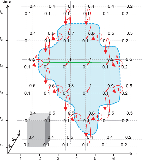
Figure 6.3. Series of six unwrapped interferograms in phase cycles. A time-space voxel is represented in gray at the bottom left. Between dates t2 and t5, there are phase differences exceeding a 0.5 cycle where residues arise. In 3D, these “spatial” residues are linked to neighboring “space-time” residues and form a closed loop (the dashed blue curve). Here, the surface cut is represented in light blue. It is contained in a plane and bounded by the loop. For a color version of this figure, see www.iste.co.uk/cavalie/images.zip
The quasi-L∞-norm 3D algorithm (Hooper and Zebker 2007) processes interferometric time series, and the spatial sampling can be either regular or irregular (e.g. due to persistent scatterer processing). In the latter case, the voxels are wedge-shaped 3D elements instead of cubes. This algorithm identifies all residues, then links the residues to form a partial or closed residue loop. If the loop is closed, the surface cut can be defined as explained earlier. If it is not, a process tries to pair the partial loops in order to minimize the total cut surface. Once all the surfaces are defined, the integration is realized by a flood-fill algorithm that does not cross any surface cut. Hooper and Zebker show that this algorithm works well on simulated and real data.
6.2.4. Least-squares method
Ghiglia and Romero (1994) developed a fast unwrapping algorithm based on least-squares minimization, i.e. the L2 norm, the first version being unweighted and the second being weighted. First, the wrapped phase gradient is computed as in equation [6.6]. Following the notations defined in section 6.2.1, the least-squares solution is the field Φ that minimizes the minimization function F of equation [6.10] with p = 2 and uniform weights. Hunt (1979) has shown that the least-squares solution can be written as:
If the known right-hand side of the equation is noted ρ(i, j), equation [6.11] can be rewritten as a discrete equivalent of Poisson’s equation:
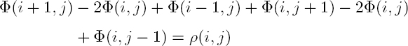
The left-hand side of the equation is the discrete equivalent of the Laplacian operator. It should be noted that the unwrapped phase is estimated only using ρ(i, j), which can be considered as an estimate of the Laplacian of Φ from the measures Ψ. Then, the discrete cosine transform (DCT) leads to a very simple formulation of the problem, as the computation of the DCT of the exact solution DCT(Φ(i, j)) is simply rewritten:
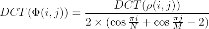
Then, the solution can be easily computed with the inverse DCT. It can be noted that this algorithm directly gives an estimate of Φ, whereas most unwrapping algorithms first evaluate ∇Φ. The weighted version of this algorithm is an iterative process also based on the DCT.
Although very fast and simple to implement, this algorithm has two drawbacks. First, the L2-norm is not the most appropriate because it has the property of distributing the errors, causing error spreading. Second, when the interferogram has a non-zero fringe rate, the slope of the phase is underestimated, as detailed in Bamler et al. (1998) and summarized hereafter. Let us first assume that there is no slope on the interferogram; it is then reasonable to assume that the unwrapped phase gradient ∇Φ is centered on zero. Due to the wrapping operation to [−π, π], if Δφi > π, then ![]() underestimates Δφi by −2kπ, k ∈ N∗ (here, i is the index corresponding to the direction of the gradient and is valued 1 or 2). In contrast, if Δφi < −π, then
underestimates Δφi by −2kπ, k ∈ N∗ (here, i is the index corresponding to the direction of the gradient and is valued 1 or 2). In contrast, if Δφi < −π, then ![]() overestimates Δφi by 2kπ, k ∈ N∗. Statistically,
overestimates Δφi by 2kπ, k ∈ N∗. Statistically, ![]() underestimates ΔΦ as often as it overestimates it with a significant error of ±2kπ. Let us now assume that there is a global positive slope α in the line direction on an interferogram (or a part of it); Δ1Φ is then centered on α > 0. Consequently, there are more pixels where Δ1Φ > π than where Δ1Φ < −π. Finally,
underestimates ΔΦ as often as it overestimates it with a significant error of ±2kπ. Let us now assume that there is a global positive slope α in the line direction on an interferogram (or a part of it); Δ1Φ is then centered on α > 0. Consequently, there are more pixels where Δ1Φ > π than where Δ1Φ < −π. Finally, ![]() underestimates Δ1Φ more often that it overestimates it which introduces a bias. In summary, whatever the sign of α, the phase gradient error has a non-zero expectation if α ≠ 0:
underestimates Δ1Φ more often that it overestimates it which introduces a bias. In summary, whatever the sign of α, the phase gradient error has a non-zero expectation if α ≠ 0:
Globally, the underestimation of | Δφi | leads to a reduced fringe rate for ![]() compared to Φ. Let us note that this underestimation also implies that the solution
compared to Φ. Let us note that this underestimation also implies that the solution ![]() is non-congruent with Φ. Although proper weighting can lessen this effect, it would be impossible to tailor perfect weighting such that this underestimation effect would never occur. The least-squares approach thus leads to an imperfect estimate of the unwrapped phase. Figure 6.2d confirms that the least-squares algorithm does not perform as well as other algorithms.
is non-congruent with Φ. Although proper weighting can lessen this effect, it would be impossible to tailor perfect weighting such that this underestimation effect would never occur. The least-squares approach thus leads to an imperfect estimate of the unwrapped phase. Figure 6.2d confirms that the least-squares algorithm does not perform as well as other algorithms.
6.2.5. Network-based approaches
6.2.5.1. The MCF algorithm and its 3D generalization
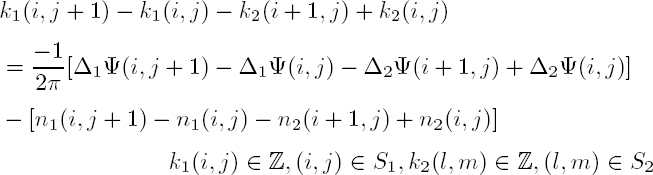
The minimum cost flow algorithm was first described in its original 2D version by Costantini (1998). It was then generalized to take into account the temporal dimension, as well as sparse data. The aim is to find the gradient fields of Φ from those of Ψ. First, two integer fields n1 and n2 are usually chosen such that:
Then, the discrete partial derivative residuals k1 and k2 are defined as:
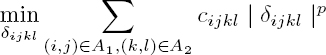
k1 (respectively, k2) should be zero almost everywhere when Δ1Φ(i, j) ∈ [−π, π[ (respectively, Δ2Φ(i, j)) and if n1 fulfills equation [6.15] (respectively, when n2 fulfills equation [6.16]). The points where k1 or k2 are non-zero correspond to branch cuts (Goldstein et al. 1988). Then, the idea is to estimate these residuals so that the gradient fields of Φ fulfill the irrotational property. This is done through a constrained minimization of a function weighted by confidence maps c1(i, j), (i, j) ∈ S1 and c2(i, j), (i, j) ∈ S2, expressing the confidence on k1 (respectively, k2). The function to be minimized is written:
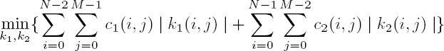
subject to the constraints:
Condition [6.20] expresses the constraint that ∇Φ must fulfil the irrotational property. However, the function to minimize in equation [6.19] is nonlinear due to the absolute values. Thus, the problem is rewritten to get rid of the absolute values. It should be noted that the variables k1(i, j), (i, j) ∈ S1 and k2(i, j), (i, j) ∈ S2 can be considered as flows on non-oriented edges between any pair of neighboring pixels. As these flows can be positive or negative, the function to minimize should be applied on the absolute values of these flows. The variable k1(i, j) is in fact “replaced” by two positive variables: ![]() Thus, a single edge between two neighboring pixels is replaced by two oriented edges with opposite directions. For example,
Thus, a single edge between two neighboring pixels is replaced by two oriented edges with opposite directions. For example, ![]() is the positive flow from node (i, j) to node
is the positive flow from node (i, j) to node ![]() is the positive flow from node (i + 1, j) to node (i, j). With these new variables, the problem becomes a minimum cost network flow problem that can be solved by dedicated algorithms. In order to limit processing time, the algorithm is applied on sub-blocks of the image with sufficient overlap. While processing a new sub-block, additional constraints from already processed blocks are applied on the overlapping parts. This algorithm generally gives good performance (see Figure 6.2e), even if some parts of the interferogram are incorrectly unwrapped in this example.
is the positive flow from node (i + 1, j) to node (i, j). With these new variables, the problem becomes a minimum cost network flow problem that can be solved by dedicated algorithms. In order to limit processing time, the algorithm is applied on sub-blocks of the image with sufficient overlap. While processing a new sub-block, additional constraints from already processed blocks are applied on the overlapping parts. This algorithm generally gives good performance (see Figure 6.2e), even if some parts of the interferogram are incorrectly unwrapped in this example.
This algorithm has been generalized for sparse data where pixels are selected if their coherence is greater than a given threshold (Costantini and Rosen 1999). A Delaunay triangulation is then performed on the selected pixels. The generalization of MCF to sparse data then consists of imposing the irrotational property of the gradient of Φ to each elementary cycle of the Delaunay triangulation, instead of the classical square cycle shown in Figure 6.1.
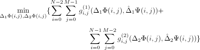
Pepe and Lanari (2006) generalized the MCF algorithm in order to simultaneously unwrap a whole stack of multi-temporal interferograms: this algorithm is called extended minimum cost flow (EMCF). In the temporal dimension, the acquisitions are represented in the classical T×B⊥ plane, where T is time and B⊥ is the perpendicular baseline. Edges on this plane represent the interferograms of the database. The unwrapping is performed in two steps. In the first step, each arc of the Delaunay triangulation in the spatial domain is unwrapped in the T × B⊥ dimension. More precisely, let us consider an arc between two neighboring pixels A and B in the spatial subset. The aim is to retrieve the unwrapped phase difference between these pixels in each interferogram. If there are M interferograms, the vector of the unwrapped phase differences between A and B is noted δΦ = (δΦ0, δΦ1, .., δΦM−1)5 and the vector of wrapped phase differences δΨ = (δΨ0, δΨ1, .., δΨM−1). Then, a parametric model m for the vector δΦ is introduced in order to help the unwrapping procedure. This model depends on two parameters (for each arc), namely Δz and Δv, which are the differential of elevation errors and the differential velocity between A and B. Then, the unwrapped vector is:
where K is a vector of integers. The aim is then to minimize:
However, instead of constraining the irrotational property on the azimuth/range plane, this constraint is imposed on the T × B⊥ plane. The elementary cycles are then the triangles formed in this plane by the database graph. If the three arcs of such a triangle are noted α, β and γ6, then equation [6.22] is minimized, subject to constraints on kα+kβ +kγ. It should be noted that the introduction of the parametric model aims at decreasing the value of the kj by removing the predictable part of δΦ. Finally, the first step gives a first estimate of the time series of the phase differences for each arc of the spatial triangulation. In the second step, the classical MCF spatial unwrapping algorithm is performed for each interferogram, beginning with the estimate given by the first step. The weights of equation [6.19] (in its irregular sampling version) are computed according to the quality of the temporal unwrapping, where greater weights are given to arcs whose temporal unwrapping is reliable. Pepe and Lanari show with simulated and real data that the EMCF performs better than classical MCF applied separately to each interferogram. This approach has been generalized to full-resolution interferograms (Pepe et al. 2011).
6.2.5.2. Redundant finite difference integration and phase unwrapping algorithm
Costantini et al. (2012) proposed a generalized formulation that can be applied to data regularly or sparsely sampled in the spatial and temporal domains; this elegant formulation is called the redundant finite difference integration and phase unwrapping algorithm. In contrast to the EMCF and the 3D stepwise algorithm alternating 1D and 2D (see section 6.2.5.3), this approach unwraps the data in the full 3D domain at once. The authors consider two graphs: the first one, (S1,A1), where nodes are in S1 and arcs are in A1, represents the space domain; the second one, (S2,A2), is the time domain. For each graph, arcs not only link closest neighbors like in a Delaunay triangulation but some supplementary links between close nodes are also considered. Then, instead of working on phase differences between neighboring pixels, the authors consider a double difference of phase in space and time, namely ![]() where (i, j) ∈ A1 and (k, l) ∈ A27. This double difference is considered because it is reasonable to assume that its absolute value is smaller than π in most cases, especially if an adequate model can be subtracted. Let (S1, T1) (respectively, (S2, T2)) be a spanning tree of (S1, A1) and B1 (respectively, B2) its strictly fundamental cycle basis8. If
where (i, j) ∈ A1 and (k, l) ∈ A27. This double difference is considered because it is reasonable to assume that its absolute value is smaller than π in most cases, especially if an adequate model can be subtracted. Let (S1, T1) (respectively, (S2, T2)) be a spanning tree of (S1, A1) and B1 (respectively, B2) its strictly fundamental cycle basis8. If ![]() are preliminary estimates of
are preliminary estimates of ![]() then the aim is to minimize:
then the aim is to minimize:
subject to the constraints:

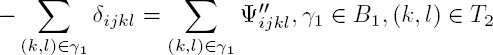
The last two constraints are irrotationality constraints in time and space. This formulation has the notable advantage of treating the time and space dimensions similarly. The originality of this method is that it makes it possible to consider the cycles in the temporal domain for each arc in the space domain and the cycles in the space domain for each arc in the time domain. Costantini et al. then study the influence of the connectivity of the graphs on phase unwrapping performance. The higher the connectivity is, the greater the redundancy. Redundancy either in the spatial domain or the time domain is shown to improve phase unwrapping performance.
6.2.5.3. Stepwise 3D algorithm and its adaptation in StaMPS software
Hooper and Zebker (2007) proposed an algorithm called the stepwise 3D algorithm that first unwraps in the temporal domain and then in the spatial domain, as in the EMCF algorithm. In the temporal domain, the differential phase between two neighboring pixels on an edge is considered and temporally unwrapped by temporal low-pass filtering, with the assumption that the double difference does not exceed π in absolute value. These first estimates are then the initial solution of the spatial unwrapping of each interferogram where any 2D unwrapping algorithm may be used. Let us note that the main steps of this algorithm are very similar to those of EMCF. Hooper (2010) implemented a variant of this last algorithm in the StaMPS software. The first step remains unchanged. The second step uses the statistical-cost network-flow algorithm for phase unwrapping (SNAPHU) for 2D unwrapping (see section 6.2.5.4). However, the statistical costs are derived from the first step.
6.2.5.4. SNAPHU
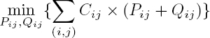
SNAPHU is a widely used, freely released 2D algorithm (Chen and Zebker 2001). Preliminary developments and explanations are given by Chen and Zebker (2000). First, the authors argue that the MCF algorithm is an L1 algorithm for which multiple-cycle discontinuities (which may arise in layover areas) are difficult to estimate, and thus that L0 pseudo-norm should be preferred as it is more adapted to the experimental content of many SAR interferograms. Indeed, multiple-cycle discontinuities are penalized by the L1 norm compared to the L0 pseudo-norm. The classical cost cycle algorithm (Ahuja et al. 1993) solves the minimum cost flow problem in the L1 norm framework with an iterative implementation. The dynamic cost cycle canceling (DCC) algorithm is a variant of the former in the L0 pseudo-norm framework. In both algorithms, costs per unit of flow are associated with any arc. In the original algorithm, these costs remain constant throughout the iterations, whereas in the DCC algorithm, the unit costs vary during the iterations, hence the “dynamic” update of the arcs costs. The DCC algorithm performs well (see Figure 6.2f), but the authors then generalize the L0 framework by replacing the weighted distance between ![]() in the minimization function with a function of these variables in the SNAPHU method (see Figure 6.2g). Precisely, the minimization function of equation [6.10] is rewritten:
in the minimization function with a function of these variables in the SNAPHU method (see Figure 6.2g). Precisely, the minimization function of equation [6.10] is rewritten:
where subscript or superscript 1 (respectively, 2) corresponds to the range (respectively, azimuth) direction. SNAPHU’s aim is to estimate the maximum a posteriori (MAP) solution ![]() given the measurements
given the measurements ![]() As the measurements are assumed to be independent, the MAP is equivalent to the maximization of the sum of the conditional log probabilities of
As the measurements are assumed to be independent, the MAP is equivalent to the maximization of the sum of the conditional log probabilities of ![]() The coherence of the interferogram is noted ρ, and the mean intensity of the two images forming the interferogram is noted I. If
The coherence of the interferogram is noted ρ, and the mean intensity of the two images forming the interferogram is noted I. If ![]() denotes the conditional probability of Φ given Ψ, then the cost functions
denotes the conditional probability of Φ given Ψ, then the cost functions ![]()
Several remarks should be made about these last equations. First, the functions ![]() vary for each pixel (i, j), as the conditional probabilities depend on the a priori distribution of Φ on each pixel, as detailed later on. Second, for a given pixel,
vary for each pixel (i, j), as the conditional probabilities depend on the a priori distribution of Φ on each pixel, as detailed later on. Second, for a given pixel, ![]() differ, as specific phase distributions in range and in azimuth are taken into account. The core of SNAPHU is its automatic definition of the cost functions (given a few user-tuned parameters) from ρ and I.
differ, as specific phase distributions in range and in azimuth are taken into account. The core of SNAPHU is its automatic definition of the cost functions (given a few user-tuned parameters) from ρ and I.
The prior distribution of ΔΦ takes into account the signal component and the noise component. The noise distribution depends on the coherence of the interferogram, whereas the signal distribution depends on the content of the interferogram. In their original paper, Chen and Zebker (2001) propose two cases, although the work may be adapted to other cases. The first is a “topographic interferogram”, i.e. an interferogram from which a DEM would be estimated. The second aims at measuring deformation on a differential interferogram due to an earthquake, with a possible high fringe rate. For the topographic case, the model takes into account I, as high-intensity pixels often correspond to layover areas where ΔΦ may take high values. It also takes into account the coherence, as low-coherence areas may also be prone to high values of ΔΦ. For the deformation case, low coherence may correspond to a sharp fringe rate and thus high values of ΔΦ. For both cases, if there is no hint that ΔΦ may be high, the cost function is a parabola centered around the expected value of ΔΦ, which is similar to the L1 norm. However, if I or ρ indicate that ΔΦ may attain high values due to layover or a high deformation rate, then the cost function has two shelves extending the range of possible values for ΔΦ “without extra cost”, which is similar to the L0 pseudo-norm. Moreover, SNAPHU only allows congruent solutions.
This approach has been generalized for large interferograms (Chen and Zebker 2002), which are cut into smaller individually unwrapped tiles. Then, phase offsets between regions are computed in order to obtain the whole interferogram.
6.2.5.5. Edgelist phase unwrapping
Shanker and Zebker (2010) proposed edgelist phase unwrapping, an algorithm to unwrap data in 3D that is similar to the EMCF algorithm but with another formulation. They consider N data points in the 2D or 3D domain (in 3D, N is the total number of pixels of the whole time series). For data points i, ni is the integer such that Φi = Ψi + 2 × π × ni, with Ψi (respectively, Φi) being the wrapped (respectively, unwrapped) phase. Considering an edge (i, j) between data points i and j, the integer Kij is the flow on this directed edge. Similar to the MCF formulation, Kij is rewritten as the difference between two positive numbers (depending on the direction of the flow on the edge) as: Kij = Pij − Qij. The MCF algorithm searches for the optimal Pij and Qij, whereas edgelist phase unwrapping also searches for the optimal ni. If Cij is the weight relative to the edge (i, j), then the function to minimize is:
subject to the constraints:
This minimization is solved by linear programming. As pointed out by the authors, the constraint is now on edges instead of loops, hence the name “edgelist”. Although the number of unknowns is greater than that in the EMCF formulation, this formulation has some advantages: it is equivalent in 2D or 3D as the data points may belong to the same interferogram or not. Moreover, additional constraints from external data such as GPS can be added without any effect on the algorithm. The authors show with a time series for San Andreas Fault that the algorithm performs well despite the sharp discontinuity across the fault.
6.2.6. Methods for correcting unwrapping errors
Regardless of the algorithm used, unwrapping errors can occur; for example, where topography is sharp, producing high fringe rates. There are also several unwrapping errors that can arise in the borders of interferograms, as there are fewer paths to link pixels on the borders to other pixels in the center of the interferogram. Such problems have been identified by several authors; for example, Chen and Zebker (2000). Although some techniques for correcting unwrapping errors can be applied to single interferograms, most of them are applied to temporal series of interferograms. Next, we first present a method applicable to a single interferogram and then methods exploiting the redundancy of the network.
6.2.6.1. Bridging scheme applicable to single interferograms
Unwrapping errors usually produce whole regions where the error spreads: each region is unwrapped well, but there is a 2kπ offset between them, k ∈ Z∗. Visual inspection of interferograms usually allows identification of such regions. One possibility is to then manually segment these regions and add the proper number of cycles to correct the unwrapping error by creating a “bridge” between neighboring regions and measuring the phase difference across the bridge. However, this process is highly time-consuming, especially for long time series. Another possibility is to discard interferograms where unwrapping errors are visible, at the expense of a poorer database. Yunjun et al. (2019) presented an approach to automatize the bridging scheme that can be applied on a single interferogram: the regions are automatically segmented, linked by bridges and their offsets are corrected. The authors showed good results with a synthetic interferogram. This approach is interesting when several parts of an interferogram cannot be linked; for example, when distinct islands are within the frame of the study area.
6.2.6.2. Error correction applied to InSAR time series
Biggs et al. (2007) observed that the closure phase on triplets of interferograms help identify unwrapping errors. A triplet is in fact the shortest closed loop in the temporal domain. The closure phase is defined in equation [6.32] and extensively described in section 6.3. If there is an unwrapping error in one of the interferograms of the triplet, then the closure is close to 2kπ, k ∈ Z∗. The closure then indicates that one of the interferograms is incorrectly unwrapped. Based on this property, several unwrapping error correction methods have been developed. It should be noted that knowledge of the closure alone is insufficient to determine which one of the three interferograms is badly unwrapped. Biggs et al. (2007) proposed the visual inspection of each of the three interferograms to determine which one is incorrectly unwrapped. Following this, other methods were developed to automatize the correction process. It should be noted that 3D unwrapping algorithms such as Costantini et al.’s (2012) fulfill the phase closure condition by definition, which is optimal. In contrast, unwrapping error-correction algorithms a posteriori correct errors due to 2D unwrapping that may have been overlooked by 3D approaches.
Hussain et al. (2016) adapted the StaMPS unwrapping algorithm described in section 6.2.5.3 in order to automatically correct unwrapping errors on a time series of interferograms. This last algorithm is used iteratively, but between each iteration, a cost is attributed to each edge in the following way. The closure phase for a closed loop of interferograms is computed for every pixel in every interferogram. The pixel is labeled as correctly (respectively, incorrectly) unwrapped if its closure is smaller (respectively, greater) than a given threshold. The labels of the two pixels of an edge determine the cost attributed to the edge: the higher the cost (i.e. the more reliable the unwrapping), the more difficult the change of the phase difference on this edge will be at the next iteration. The authors showed that this technique decreased the number of incorrectly unwrapped pixels.
Yunjun et al. (2019) presented another approach based on the analysis of closure phase for triplets. Given a time series of interferograms, a vector of integers representing the number of cycles of the error is associated with each pixel. This vector should minimize the L2 norm of the closure for all triplets of the time series. However, as the solution is not unique, a regularization term constrains the variations of this vector of integers. The authors show with a simulated database that the number of unwrapping errors significantly decreases, especially when the redundancy of the network increases, as in the approach developed by Costantini et al. (2012). As it excludes the regularization term, this approach is pixel-based.
Still based on triplet closure phase, Benoit et al. (2020) proposed an algorithm called the correction of phase unwrapping errors (CorPhU) algorithm. In contrast to the preceeding methods, which are pixel-based, this method identifies incorrectly unwrapped regions. Then, for each region, two indices are computed to determine which of the three interferograms is badly unwrapped: first, the flux between the borders of the region and a reference region is determined, which is a priori correctly unwrapped9; second, each interferogram may belong to several triplets and it is then possible to compute the mean closure for all these triplets. For a badly unwrapped interferogram, both the flux and the mean closure should be anomalous. The comparison of these indices for the three interferograms helps in identifying which interferogram is incorrectly unwrapped. The authors show with real and simulated data that the number of unwrapping errors significantly decreases.
Finally, in the NSBAS chain presented in Chapter 5, an unwrapping error correction process is performed during the inversion of the time series, which is pixel based. If the residual between inverted and original interferograms is large, then the interferogram may be badly unwrapped. The time-series inversion is computed again with a low confidence weight for such interferograms and the process is repeated iteratively until convergence of the inversion.
6.2.7. Summary and comparison
As can be seen in the preceeding sections, InSAR phase unwrapping has given rise to a great number of methods. An interesting comparison of some 2D algorithms is given by Chen and Zebker (2000), especially the difference between L0 and L1 norms. Figure 6.4 shows an overview of the principal methods cited in this chapter. Globally, three families appear. First, the residue-cut tree algorithm has been enhanced and generalized in 3D. Second, the network-based methods deriving from the MCF algorithm are preponderant, as different teams worked on these approaches and generalized them to 3D. Third, the weighted least-squares algorithm has not been generalized to our knowledge, probably due to the problem of fringe rate underestimation described in section 6.2.4.
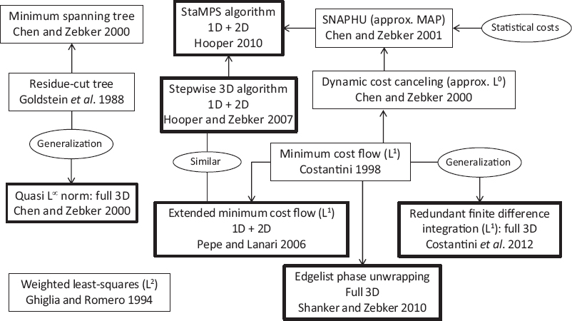
Figure 6.4. Overview of the principal phase unwrapping methods described in this section and their relationships. Two-dimensional algorithms are in thin rectangles and 3D ones in bold rectangles
With regard to 3D approaches, some are alternating 1D and 2D approaches, whereas others really consider the whole 3D problem at once, noted as “full 3D” in Figure 6.4. Thus, the quasi-L∞ 3D algorithm is the strict 3D generalization of the residue-cut tree algorithm and the redundant finite difference integration algorithm is the strict generalization of the original MCF algorithm. By “strict generalization”, we mean that all dimensions in 3D are equivalent, which is not the case for 1D + 2D methods. Edgelist phase unwrapping is part of the network-based family but differs from MCF, as constraints apply on edges rather than on loops. Finally, SNAPHU introduced a new way of weighting the minimization function by introducing statistical costs, which changed the problem from Lp-norm formulation to MAP formulation. A striking feature of the evolution of unwrapping methods is the growth of the network-based family. In our opinion, this is due to data increases and the capacity of this family to fully exploit data redundancy. Although the phase unwrapping problem is difficult and still a subject of research, redundancy should be one of the keys to solving this problem with well-adapted heuristics.
6.3. The (re)discovery of closure phases and their implications for SAR interferometry
The presence of statistical non-zero closure phases has been recognized in SAR interferometry since the development of triangulation methods (Monti Guarnieri and Tebaldini 2008). However, the discovery of physical non-zero closure phases is more recent (De Zan et al. 2012). This is somewhat surprising since the phenomenon is well-known in other fields, such as astronomy and, moreover, fundamentally invalidates well-established models for phase interpretation in multi-looked SAR interferograms and can strongly bias the deformation results. The basic equations we have been using for a long time (e.g. equations [4.5] and [5.1]) may look like crude approximations in the presence of closure phases, especially as we strive towards increased geodetic precision. At the same time, closure phases indicate a new world of physical phenomena that we will be able to observe.
6.3.1. Introduction to closure phases
With three SAR images, it is possible to generate three interferograms. The closure phase is the circular combination of the three interferometric phases:
For single pixels, the closure phase is always zero, as we can easily check. However, for multi-looked interferograms, there is no reason for the closure phase to be zero, contrary to common expectations. Consequently, to explore an interesting field, from now on we will assume that the interferometric phase is taken after a multi-look operation “< · >” on the complex interferogram, for example:
The superscript W on the phase indicates that the phase is wrapped in this equation. With this notation, we could write the closure phase directly as the phase of a triple product:
Non-zero closure phases can result from very diverse mechanisms: first, we should clearly distinguish purely statistical explanations from physical explanations. Statistical misclosure occurs every time the coherence magnitude is smaller than 1, i.e. all the time in real situations. Averaging more pixels, if possible, will reduce the statistical misclosure. Different triangulation algorithms have dealt with this kind of closure phase: Chapter 5 lists a number of such algorithms.
The second kind of misclosure is more fundamental and resists stronger multi-looking, i.e. larger spatial averaging. It is an essential type of inconsistency that requires some physical interpretation. From this perspective, the closure phase is actually a novel and interesting physical observable, especially considering that it is not sensitive to common interferometric signals, such as atmospheric delays or surface motion, as should become clear in the following.
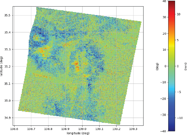
Figure 6.5. The closure phase corresponding to three ALOS-2/PALSAR-2 acquisitions over Japan, acquired on May 7, 2015, July 16, 2015, and August 27, 2015. Mt. Fuji is recognizable in the northwest corner of the image. For a color version of this figure, see www.iste.co.uk/cavalie/images.zip
Figure 6.5 shows an example of a full-scene closure phase. It has been derived from ALOS-2/PALSAR-2 data10 (L-band) acquired over Japan. The Izu peninsula (north–south) occupies the center of the image. To the east and west, it is possible to recognize the water areas, displaying zero-mean, noisy closure-phase.
Finally, the presence of closure phases forces us to reconsider the phase estimation in an interferometric stack of SAR images. The choice and weight given to the various interferograms can potentially lead to very different results in the reconstruction of the phase history. The phase triangulation algorithms were meant to deal with statistical misclosure, not with physical misclosure. Surprisingly, at least to a point, the triangulation algorithms display some robustness to physical misclosures too.
6.3.2. Mathematical properties of closure phases
Initially, the reader could be surprised in hearing that phases are always perfectly closed for single pixels and almost never for spatial averages of interferograms. The clean explanation lies in the nonlinearity of the arc-tangent operation: there is actually no reason why a linear operation in the real and imaginary part of the interferogram – like multi-looking – should commute with a nonlinear function.
The false zero-closure-phase expectation is also supported by the usual models for the phase, which describe the phase as a pure distance to a single target (equation [4.1]). Many physical signals indeed obey the piston-like paradigm (Zwieback et al. 2016), such as tropospheric delays, and might easily suggest a hasty generalization.
Closure phases are invariant to phase calibration11, i.e. closure phases do not change if we multiply each image by a phasor exp [jφn]. Checking this is trivial, as the effect will be opposite signs on two interferograms of the triplet.
Closure phases as a robust invariant are not unique. Astronomers also exploit closure amplitudes, which are a particular combination of what we would call correlation magnitudes (Chael et al. 2018).
A couple of simple properties define a circular permutation symmetry:
and an odd symmetry for anti-circular permutations:
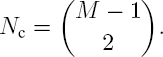
If the total number of closure phases in a stack with M images is ![]() the number of independent closure phases is only quadratic in M (De Zan et al. 2015; Zwieback et al. 2016):
the number of independent closure phases is only quadratic in M (De Zan et al. 2015; Zwieback et al. 2016):
It is possible to see this by noting that the Nc closure phases of the form Φ1,n,k with k > n > 1 constitute a basis. They are enough to express any closure phase:
whereas each Ψ1,n,k is necessary as it is the only element containing the interferometric phase φn,k.
Nc is therefore the dimension of the inconsistent (non-zero closure) subspace; adding the M − 1 consistent phases (e.g. all relative to a reference), we get:
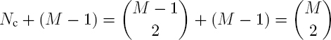
which is the total number of independent phases in the (temporal) covariance matrix of M acquisitions, considering the Hermitian symmetry.
6.3.3. Physical misclosures
The simplest scattering model that allows for non-zero closure phases is a two scatter model with independent phase variations:
Let us assume that the two scatterers a and b are zero-mean uncorrelated random variables so that E[ab∗] = 0. The expected value of the interferogram, thanks to this assumption, is:
Provided that ![]() any trajectory comprising three different values for φ(t) will generate a non-zero closure phase. The two scatterers represent different populations in the same resolution cell, with different phase histories. Sometimes, the multi-looking operation can be responsible for mixing two populations that are well separated in the image. In this special case, the closure phase would be an artifact.
any trajectory comprising three different values for φ(t) will generate a non-zero closure phase. The two scatterers represent different populations in the same resolution cell, with different phase histories. Sometimes, the multi-looking operation can be responsible for mixing two populations that are well separated in the image. In this special case, the closure phase would be an artifact.
A more general model would include many (possibly infinite) scatterers, each modeled by a zero-mean uncorrelated stochastic process with a peculiar phase history:
and real correlation ![]() where δnk is the Kronecker symbol.
where δnk is the Kronecker symbol.
The corresponding interferograms will be:
This is simply the sum of the individual interferograms corresponding to the elemental scatterers.
It is possible to find examples of physical closure phases in all frequency bands, for P-band to K-band. The mere mathematical possibility of their existence is in fact defined by a rich variety of cases. There is no single physical phenomenon that explains all observed misclosures and, in reality, different physical mechanisms will be at work simultaneously, which might complicate the retrieval of physical parameters.
This is not a new situation in SAR, where even in the ordinary interferometric phase, it is possible to recognize a plethora of contributions (deformation, topography, atmospheric propagation, etc.). It is an error to expect closure phases to derive from a single physical origin. The following sections present different physical models that can yield closure phases to clarify this concept.
6.3.3.1. A volumetric scatterer observed at different angles
This example of physical non-closure is really equivalent to the model used in astrophysics.
Let us assume that we have a volumetric scatterer ξ that statistically depends only on the vertical coordinate such that E[ξ(z)ξ∗(z′ )] = f(z)δ(z − z′ ). The function f(z) ≥ 0 then describes the expected intensity along the vertical direction.
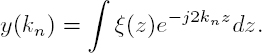
If the volume is observed under different incidence angles, the resulting images can be modeled as integrals:
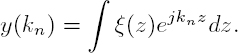
as a function of the vertical wavenumber kn, for the n-th acquisition. The interferograms will be:
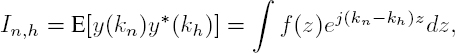
i.e. a function of the differential wavenumber kn − kh. Normalizing f(z) such that ![]() which makes it equivalent to a probability distribution, it is possible to show (De Zan et al. 2015) that for small wavenumber variations:
which makes it equivalent to a probability distribution, it is possible to show (De Zan et al. 2015) that for small wavenumber variations:
This gives a simple interpretation of the closure phase as being proportional to the skewness E[(z − E[z])3] of the scattering intensity profile f(z). This interpretation is of course shared in astronomical imaging with closure phases.
This type of closure phase mechanism can impact deformation estimation in time series where the distribution of the baselines has some structure in time, for example, if the baselines are left to drift for periods longer than the repeat pass and then are suddenly corrected. Indeed, orbital drift is not random, for example, because of atmospheric drag. In other cases, the mission plan may contemplate a certain systematic baseline variation, as in the case of the BIOMASS mission.
6.3.3.2. A simple interferometric model for soil moisture
A possible interferometric model for a soil under different moisture conditions is to think of the soil as a dielectric volume, whose permittivity ∈ varies as a function of the moisture state and soil composition (Hallikainen et al. 1985; Bircher et al. 2016). Following the Born approximation, little scatterers dispersed inside the volume will generate a backscattered field, each scatterer with amplitude and phase proportional to the incident background field (De Zan et al. 2012). The resulting model for the backscatter is very similar to the one for a volume observed at different angles:
One first difference is that the volume here is likely only a few centimeters thick. A second difference is that the vertical wavenumber kn is typically complex. It is a function of permittivity, approximately ![]() where ω is the angular frequency, μ is the dielectric permeability and ∈(n) the dielectric permittivity at the time of the nth acquisition.
where ω is the angular frequency, μ is the dielectric permeability and ∈(n) the dielectric permittivity at the time of the nth acquisition.
To derive the expected value of the interferograms, we adopt the usual assumption that ![]() and obtain:
and obtain:
The scattering profile does not have to follow any particular dependence on depth. If it is exponential, f(z) = exp(−2αz), with α ≥ 0, the integral has a simple analytical solution:
For α = 0, the formula covers also the case of a constant scattering profile.
This model seems to describe reasonably well the closure phases in L-band over bare soil, at least in the example given by De Zan et al. (2014). Inverting the soil moisture model from closure phases is not trivial; as Zwieback et al. (2017) point out, there is an ambiguity in the relation between moisture histories and the corresponding closure phases. However, with the additional help of coherence magnitudes or intensities, the inverse problem seems feasible at least for a limited sequence of acquisitions (De Zan and Gomba 2018).
In theory, moisture variations can produce a velocity bias in the time series. The bias can arise from the moisture cycle, which normally sees a sudden wetting and a slow drying. If the phase depends in a nonlinear way on moisture differences, then a fast wetting will be more than compensated by a slow drying. In the long term, by integrating short-term pairs, we should observe an apparent decrease in the distance, i.e. a motion towards the satellite. This might have been observed, but conclusive proof is still needed.
6.3.3.3. Other reasons for differential motion in a resolution cell
There are likely many other sources of differential motion in a resolution cell that can ultimately yield non-zero phase closure. For example, there could be differential motion in ice (as a function of depth) when dry ice is observed with sufficiently long wavelengths. There could be thermal expansion displacing different targets of different amounts.
Another possibility is vegetation superimposing a time-variable phase screen. If not all targets are covered by the same amount of vegetation, then there could be differences that produce non-zero closure phases. This tentative explanation is given by Ansari et al. (2021) to explain a phase bias that did no display behavior that the moisture model would predict. In this case, the prevailing small steps were biomass accumulation, i.e. delay increase.
Different sources of phase inconsistency might be present at once, and if they are generated by independent (orthogonal) mechanisms, then it is likely safe to assume that they contribute to the closure phase independently. For example, if one differential mechanism is in the time domain and the other in the Doppler domain, then the resulting closure phase would be the sum of the closure phases for each independent mechanism.
6.3.4. Implications for interferometric phase estimation
6.3.4.1. Statistical misclosure and phase triangulation algorithms
Different from physical misclosures, statistical misclosures have been recognized for a long time. The phase triangulation algorithms (e.g. Monti Guarnieri and Tebaldini 2008; Ansari et al. 2018; Michaelides et al. 2019) exploit the hypothesis of underlying phase closure to improve the phase estimates in a stack. Even if these were mostly not designed to deal with physical closure phases, they happen to usually do a good job in retrieving the phase related to long-term coherent scatterers (Ansari et al. 2021).
This is possible thanks to redundancy. The available interferograms are M(M − 1)/2, and each of them describes a time difference between only M independent acquisition times. We realize that there are many alternative paths to reconstruct the phase difference between a given pair of acquisition times. The problem is finding which paths are good and how to weight them properly.
There is a common pitfall in choosing the paths: letting coherence drive the choice. Indeed, we can show that many high-coherence steps might be worse than a single or a few low-coherence steps, depending on the coherence scenario. In theory, the phase triangulation algorithms deal with this complexity in an optimal way. In practice, they have limitations related to limited or biased knowledge of the temporal coherence structure.
6.3.4.2. Biases everywhere
A particularly dangerous situation arises when the physical closure phases present some particular structure in time, for example, when they tend to be always biased in one direction. This can happen with any of the physical phenomena analyzed above. For instance, the closure phases with three images in a successive acquisition order could tend to have the same sign in the moisture model, if moisture increase is a rare event, and moisture decrease can be observed over many repeat cycles. Similar reasoning can be applied for any of the mentioned possible physical mechanisms.
Another, more abstract, perspective is given by considering the following complex coherence model:
This is a model with two scatterers, one stable and the other decorrelating (with temporal characteristic τb) and simultaneously moving (with “velocity” fb). This kind of behavior was observed by Ansari et al. (2021). The model should be understood as if we had compensated a phase so that the first scatterer appears not to have moved at all; the second scatterer shows its relative or residual motion with respect to the first. The Kronecker δ is just there to guarantee a coherence of 1 for the auto-interferogram.
We might find it disturbing that the second scatterer appears to move indefinitely, but this is accommodated by the coherence loss, under which a steady state might be continuously recovered under the invisibility cloak of decorrelation.
According to this model, long-term interferograms will see the “correct” velocity of the first scatterer, since the second scatterer is completely decorrelated. However, short-term interferograms will see another apparent motion, partially biased by the motion of the second scatterer. Considering interferograms of different time lags, the estimated velocity might be very different. Figure 6.6 displays the velocity bias as a function of the temporal baseline for a certain choice of the parameters (based roughly on C-band observations over Sicily reported by Ansari et al. (2021)). In this example, the bias can reach about 10 mm/year for a short temporal baseline and is less than 1 mm/year only when the separation is greater than 30 days.
The reality is likely more complex that the simple model presented here. There might be different contributions with different time constants and different apparent velocities. If a long-term coherent scatterer is present, it can act as an anchor to keep the estimates from drifting. This is done implicitly by using a full-covariance estimator or explicitly by avoiding short-term interferograms, as in the study by Daout et al. (2020).
It might be possible to quantify the bias for short-term interferograms by estimating closure phases with very asymmetric temporal lags, i.e. with two long arms and one short arm. In the long arms, the bias will probably be very small so that the closure phase would be representative of the short-arm bias. Of course, this requires some care, since in the long arms, the decorrelation will be strong.
6.3.4.3. Outlook: multi-frequency and polarimetry
Closure phases remind us that the phase of the scattered signal does not reflect a simple delay, and this can have significant consequences on the deformation products and complex implications for the processing algorithms. A deeper understanding of the scattering mechanisms requires more physical modeling, which will have to explain backscatter and phase behavior across different frequencies and polarizations.
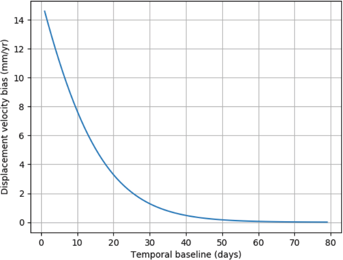
Figure 6.6. Velocity bias as a function of temporal baseline for the model in equation [6.60] for γa = 0.38, γb = 0.18, τb = 11 days, fb = 0.03 rad/day
6.4. Acknowledgments
We thank Professor Mario Costantini, Professor Paco López-Dekker and Mrs Yan Yuan for their careful reviews and comments that helped to improve this chapter.
6.5. References
Ahuja, R.K., Magnanti, T.L., Orlin, J.B. (1993). Network Flows: Theory, Algorithms, and Applications. Prentice Hall, Englewood Cliffs.
Ansari, H., De Zan, F., Bamler, R. (2018). Efficient phase estimation for interferogram stacks. IEEE Transactions on Geoscience and Remote Sensing, 56(7), 4109–4125.
Ansari, H., De Zan, F., Parizzi, A. (2021). Study of systematic bias in measuring surface deformation with SAR interferometry. IEEE Transactions on Geoscience and Remote Sensing, 59(2), 1285–1301.
Bamler, R. and Hartl, P. (1998). Synthetic aperture radar interferometry. Inverse Problems, 14.
Bamler, R., Adam, N., Davidson, G.W., Just, D. (1998). Noise-induced slope distortion in 2-D phase unwrapping by linear estimators with application to SAR interferometry. IEEE Transactions on Geoscience and Remote Sensing, 36(3), 913–921.
Benoit, A., Pinel-Puysségur, B., Jolivet, R., Lasserre, C. (2020). CorPhU: An algorithm based on phase closure for the correction of unwrapping errors in SAR interferometry. Geophysical Journal International, 221(3), 1959–1970.
Biggs, J., Wright, T., Lu, Z., Parsons, B. (2007). Multi-interferogram method for measuring interseismic deformation: Denali Fault, Alaska. Geophysical Journal International, 170(3), 1165–1179.
Bircher, S., Demontoux, F., Razafindratsima, S., Zakharova, E., Drusch, M., Wigneron, J.-P., Kerr, Y.H. (2016). L-band relative permittivity of organic soil surface layers – A new dataset of resonant cavity measurements and model evaluation. Remote Sensing, 8(12), 1–17.
Chael, A.A., Johnson, M.D., Bouman, K.L., Blackburn, L.L., Akiyama, K., Narayan, R. (2018). Interferometric imaging directly with closure phases and closure amplitudes. The Astrophysical Journal, 857(1), 23.
Chen, C.W. and Zebker, H.A. (2000). Network approaches to two-dimensional phase unwrapping: Intractability and two new algorithms. Journal of the Optical Society of America A, 17(3), 401–414.
Chen, C.W. and Zebker, H.A. (2001). Two-dimensional phase unwrapping with use of statistical models for cost functions in nonlinear optimization. Journal of the Optical Society of America A, 18(2), 338–351.
Chen, C.W. and Zebker, H.A. (2002). Phase unwrapping for large SAR interferograms: Statistical segmentation and generalized network models. IEEE Transactions on Geoscience and Remote Sensing, 40(8), 1709–1719.
Costantini, M. (1998). A novel phase unwrapping method based on network programming. IEEE Transactions on Geoscience and Remote Sensing, 36(3), 813–821.
Costantini, M. and Rosen, P. (1999). A generalized phase unwrapping approach for sparse data. IGARSS’99, 1, 267–269.
Costantini, M., Malvarosa, F., Minati, F. (2012). A general formulation for redundant integration of finite differences and phase unwrapping on a sparse multidimensional domain. IEEE Transactions on Geoscience and Remote Sensing, 50(3), 758–768.
Daout, S., Dini, B., Haeberli, W., Doin, M.-P., Parsons, B. (2020). Ice loss in the northeastern Tibetan Plateau permafrost as seen by 16 yr of ESA SAR missions. Earth and Planetary Science Letters, 545, 116404.
De Zan, F. and Gomba, G. (2018). Vegetation and soil moisture inversion from SAR closure phases: First experiments and results. Remote Sensing of Environment, 217, 562–572.
De Zan, F., Parizzi, A., Prats, P. (2012). A proposal for a SAR interferometric model of soil moisture. IEEE International Geoscience and Remote Sensing Symposium, 630–633.
De Zan, F., Parizzi, A., Prats-Iraola, P., López-Dekker, P. (2014). A SAR interferometric model for soil moisture. IEEE Transactions on Geoscience and Remote Sensing, 52(1), 418–425.
De Zan, F., Zonno, M., Lopez-Dekker, P. (2015). Phase inconsistencies and multiple scattering in SAR interferometry. IEEE Transactions on Geoscience and Remote Sensing, 53(12), 6608–6616.
Ferretti, A., Prati, C., Rocca, F. (2001). Permanent scatterers in SAR interferometry. IEEE Transactions on Geoscience and Remote Sensing, 39(1), 8–20.
Ghiglia, D.C. and Romero, L.A. (1994). Robust two-dimensional weighted and unweighted phase unwrapping that uses fast transforms and iterative methods. Journal of the Optical Society of America A, 11(1), 107–117.
Goldstein, R., Zebker, H.A., Werner, C. (1988). Satellite radar interferometry: Two-dimensional phase unwrapping. Radio Science, 23, 713–720.
Hallikainen, M.T., Ulaby, F.T., Dobson, M.C., El-Rayes, M.A., Wu, L.-K. (1985). Microwave dielectric behavior of wet soil – Part 1: Empirical models and experimental observations. IEEE Transactions on Geoscience and Remote Sensing, 23(1), 25–34.
Hooper, A. (2010). A statistical-cost approach to unwrapping the phase of InSAR time series. Fringe Workshop, 30 November–4 December, Frascati.
Hooper, A. and Zebker, H.A. (2007). Phase unwrapping in three dimensions with application to InSAR time series. Journal of the Optical Society of America A, 24(9), 2737–2747.
Hunt, B.R. (1979). Matrix formulation of the reconstruction of phase values from phase differences. Journal of the Optical Society of America A, 69(3), 393–399.
Huntley, J.M. (2001). Three-dimensional noise-immune phase unwrapping algorithm. Applied Optics, 40(23), 3901–3908.
Hussain, E., Hooper, A., Wright, T.J., Walters, R.J., Bekaert, D.P.S. (2016). Interseismic strain accumulation across the Central North Anatolian Fault from iteratively unwrapped InSAR measurements. Journal of Geophysical Research: Solid Earth, 121(12), 9000–9019.
Michaelides, R.J., Zebker, H.A., Zheng, Y. (2019). An algorithm for estimating and correcting decorrelation phase from InSAR data using closure phase triplets. IEEE Transactions on Geoscience and Remote Sensing, 57(12), 10390–10397.
Monti Guarnieri, A. and Tebaldini, S. (2008). On the exploitation of target statistics for SAR interferometry applications. IEEE Transactions on Geoscience and Remote Sensing, 46, 3436–3443.
Pepe, A. and Lanari, R. (2006). On the extension of the minimum cost flow algorithm for phase unwrapping of multitemporal differential SAR interferograms. IEEE Transactions on Geoscience and Remote Sensing, 44(9), 2374–2383.
Pepe, A., Euillades, L.D., Manunta, M., Lanari, R. (2011). New advances of the extended minimum cost flow phase unwrapping algorithm for SBAS-DInSAR analysis at full spatial resolution. IEEE Transactions on Geoscience and Remote Sensing, 49(10), 4062–4079.
Shanker, A.P. and Zebker, H.A. (2010). Edgelist phase unwrapping algorithm for time series InSAR analysis. Journal of the Optical Society of America A, 27(3), 605–612.
Trouvé, E., Nicolas, J.M., Maître, H. (1998). Improving phase unwrapping techniques by the use of local frequency estimates. IEEE Transactions on Geoscience and Remote Sensing, 36(6), 1963–1972.
Yunjun, Z., Fattahi, H., Amelung, F. (2019). Small baseline InSAR time series analysis: Unwrapping error correction and noise reduction. Computers and Geosciences, 133, 104331.
Zwieback, S., Liu, X., Antonova, S., Heim, B., Bartsch, A., Boike, J., Hajnsek, I. (2016). A statistical test of phase closure to detect influences on DInSAR deformation estimates besides displacements and decorrelation noise: Two case studies in high-latitude regions. IEEE Transactions on Geoscience and Remote Sensing, 54(9), 5588–5601.
Zwieback, S., Hensley, S., Hajnsek, I. (2017). Soil moisture estimation using differential radar interferometry: Toward separating soil moisture and displacements. IEEE Transactions on Geoscience and Remote Sensing, 55(9), 5069–5083.
- 1. Strictly speaking, “closure phase” refers to a measurement whereas “phase closure” refers to the principle of phase triangularity, i.e. to the nullity of closure phase. However, some authors use the expression “phase closure” instead of “closure phase” (e.g. Benoit et al. 2020).
- 2. Depending on the author, the wrapped phase may lie in [0, 2π[ instead.
- 3. If the wrapped phase lies in [0, 2π], then W (?) is defined as: W (?) = ?[2π].
- 4. If the rotational is computed in terms of the number of cycles as in Figure 6.1, then it values

- 5. In contrast to the Pepe and Lanari’s notation (2006), Φ refers to the unwrapped phase and Ψ refers to the wrapped one to ensure this chapter’s internal coherence.
- 6. These three arcs are three interferograms derived from three acquisition dates.
- 7. The notations introduced here are different from the original ones (which are more general) to ensure this chapter’s internal coherence. Φik corresponds to
 and
and 
- 8. A unique cycle (S1, T1 ∪ (i, j)) is associated with each arc (i, j) ∈ A1T1. By definition, the set B1 of all these cycles has a strictly fundamental cycle basis.
- 9. Although similar to the bridging scheme of Yunjun et al. (2019), the segmentation of the interferograms into regions unwrapped with an offset is derived from the closure phase.
- 10. The ALOS-2/PALSAR-2 data were kindly provided by the Japanese Aerospace Exploration Agency (JAXA) under the sixth Research Announcement (RA) Program.
- 11. In radio astronomy, closure phases are considered a robust estimator not affected by the local, unknown atmospheric delay.