
5
Advanced Methods for Time-series InSAR
Dinh HO TONG MINH1, Ramon HANSSEN2, Marie-Pierre DOIN3 and Erwan PATHIER3
1UMR-TETIS, INRAE, France
2Delft University of Technology, The Netherlands
3ISTerre, Grenoble, France
5.1. Introduction
Time-series InSAR analysis is a well-known technique that is used to map large-scale surface subsidence with high accuracy from space. There are two main reasons to move from traditional InSAR (i.e. based on a single image pair) to time-series InSAR: (1) it would enable the study of temporarily extended and varying phenomena and (2) it would improve the precision of surface displacement measurements. Indeed, for deformation processes that develop slowly (e.g. land compaction, interseismic deformation, reservoir pressurization, slow-moving landslides or ice flows), this technique allows us to exploit the redundancy in InSAR time-series stacks to mitigate noise and nuisance signals such as atmospheric effects, residual topography and decorrelations.
While many time-series InSAR methods have been developed in the last 20 years, most of them share similar characteristics so that they can be categorized into two types of techniques based on how they account for signal decorrelations (Ho Tong Minh et al. 2020). The first category of techniques is based on distributed scatterers (DSs) for deformation monitoring. Distributed targets occur in natural environments (meadows, fields, bare soil) where many similarly bright scatterers contribute to the information existing in a resolution cell. A common way of reducing signal decorrelations is to select interferograms with short spatial and temporal baselines (small baseline (SB) techniques). Distributed targets are plentiful, facilitating densely sampled deformation maps. However, deformation measurements of distributed targets are often lower quality and therefore require spatial filtering. The second approach is permanent/persistent scatterer (PS) InSAR techniques, which use individual scatterers that dominate the signal from within a resolution cell to track deformation through time. The well-known scattering stability is due to the fact that point-like targets are often associated with stable human-made structures such as buildings, poles and gratings, resulting in very low decorrelations. Consequently, PS techniques provide high-quality deformation information at point target locations. However, the density of PS targets is often low in non-urban areas, resulting in a sparse distribution of usable points. To overcome this, a recent advanced technique allows us to combine both PSs and DSs to overcome the sparsity of identified points for estimation (the persistent scatterer–distributed scatterer (PSDS) technique).
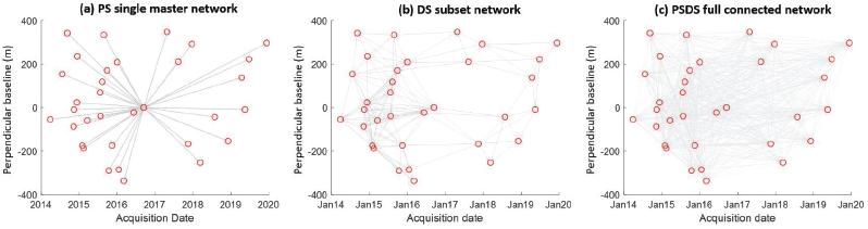
Figure 5.1. Examples of interferogram networks generated by using COSMO SkyMed data (provided by the Italian Space Agency under research project ID226) from over the Ho Chi Minh City area. (a) The single master network with permanent/persistent scatterer (PS) techniques. (b) The subset network consisting of interferograms with small temporal and spatial baselines with the small baseline subset (SBAS) technique. (c) The full network consisting of all possible interferograms with the persistent scatterer–distributed scatterer (PSDS) technique
To perform an InSAR time-series analysis, it is necessary to reconstruct the evolution of the unwrapped phase between each acquisition date. If we rely on interferograms, it is therefore necessary for all dates to be connected by interferograms. A common way to represent these connections is a graph in which the interferograms are represented by edges that link the nodes of the network, which are the SAR images plotted according to their acquisition time and perpendicular baseline. Figure 5.1 shows three examples of interferogram networks related to the different time-series techniques mentioned above. If some acquisition dates are not connected by the interferogram network, it is necessary to make more or less strong assumptions to reconstruct the phase evolution. An example is the so-called “stacking” method, which makes the strong assumption that, in each pixel, the phase evolution is linear with time. This relies on the sum of independent (i.e. not connected) interferograms to estimate a velocity map (e.g. Wright et al. 2001). However, this assumption is not acceptable in most cases, and other approaches that require access to the unwrapped phase of each interferogram are necessary.
This chapter describes the two main families of time-series InSAR techniques (SB and PSDS). It is organized as follows: the mathematical background is provided in section 5.2; methodology advancements are summarized in section 5.3; the SB technique is presented in section 5.4; and finally the PSDS technique is presented in section 5.5.
5.2. Background of time-series InSAR analysis
Let us assume that N SAR images are available. The images are co-registered on a reference/common grid. Let us assume that phase terms due to orbit and terrain topography have been estimated and compensated for. The residual phase of the unwrapped differential interferogram φn, for each acquisition n, is composed of the phase components contributed by residual topography, deformation, atmosphere and noise (Hanssen 2001):
where ![]() is the residual topographic phase;
is the residual topographic phase; ![]() is the phase due to the surface displacement;
is the phase due to the surface displacement; ![]() is the atmospheric phase screen (APS), representing the contribution of weather conditions;
is the atmospheric phase screen (APS), representing the contribution of weather conditions; ![]() is the phase noise due to all other possible contributions, such as temporal decorrelation, mis-coregistration, uncompensated spectral shift decorrelation, orbital errors, soil moisture and thermal noise; and k is an integer ambiguity number.
is the phase noise due to all other possible contributions, such as temporal decorrelation, mis-coregistration, uncompensated spectral shift decorrelation, orbital errors, soil moisture and thermal noise; and k is an integer ambiguity number.
For a point p, the residual topographic phase can be written as (Hanssen 2001):
where ![]() is the height-to-phase factor;
is the height-to-phase factor; ![]() is the residual topography or the elevation error;
is the residual topography or the elevation error; ![]() is the perpendicular baseline of the n-th image with respect to the reference image; θp is the local incidence angle; λ is the carrier radar wavelength; and Rn,p is the target–satellite distance.
is the perpendicular baseline of the n-th image with respect to the reference image; θp is the local incidence angle; λ is the carrier radar wavelength; and Rn,p is the target–satellite distance.
Without loss of generality, the phase component due to the displacement at a point p can be usefully split into two components:
where vp is the mean light-of-sight (LOS) velocity of the target; ![]() is the time-to-phase factor; tn is the temporal baseline; and μNL is the phase term due to a possible nonlinear motion.
is the time-to-phase factor; tn is the temporal baseline; and μNL is the phase term due to a possible nonlinear motion.
The APS ![]() is usually not modeled because it depends on weather conditions, but it can be reduced significantly by considering phase differences between the nearby points thanks to its spatial covariance properties (Emardson et al. 2003). The noise term
is usually not modeled because it depends on weather conditions, but it can be reduced significantly by considering phase differences between the nearby points thanks to its spatial covariance properties (Emardson et al. 2003). The noise term ![]() contains all the other phase contributions.
contains all the other phase contributions.
Most often, a linear model for the residual topography and a constant velocity are assumed. More specifically, given N − 1 unwrapped differential interferograms, for each pixel, using equation [5.1], we can write a system of N − 1 equations with two unknowns:
where ![]() is the residual phase. The problem in equation 5.4 will be linear if the integer ambiguity number k is known. Unfortunately, φn can be only observed as a wrapped phase (i.e. k is also an unknown) (Ghiglia and Pritt 1998; Hanssen 2001). PS and PSDS approaches can be carried out directly from the wrapped phase, whereas the phase input in SB analyses should be unwrapped.
is the residual phase. The problem in equation 5.4 will be linear if the integer ambiguity number k is known. Unfortunately, φn can be only observed as a wrapped phase (i.e. k is also an unknown) (Ghiglia and Pritt 1998; Hanssen 2001). PS and PSDS approaches can be carried out directly from the wrapped phase, whereas the phase input in SB analyses should be unwrapped.
5.3. A review
5.3.1. Small baseline methods for time-series analysis
The objective of this processing strategy is to establish a time series for ground displacement with the largest possible spatial coverage and density for different types of land cover. Achieving this objective depends essentially on the ability to obtain the unwrapped phase over the maximum number of pixels at the scale of a network of interferograms connecting the different dates of acquisition of the time series. This capacity quickly becomes limited in the presence of strong phase gradients and decorrelation noise (see Chapter 6). In natural environments, dominated by DSs, geometric and temporal decorrelation are two main limiting factors (see Chapter 4). The idea of the SB approach is therefore to establish a network of interferograms for which these decorrelation effects are minimized.
In early radar missions such as Radarsat-1 and JERS-1, the large variability of the perpendicular baseline and the viewing squint angle, due to poor orbital control and yaw steering capabilities (see Chapter 1), made geometrical decorrelation the main limitation. For C-band ERS and Envisat satellites that were better yaw steered but remained in an orbital tube with a diameter larger than 1 km, the perpendicular baseline was still a critical criterion to be minimized when the first InSAR time-series analysis started by the end of the 1990s. This explains the term “small baseline”; however, it is important to keep in mind that other criteria are applied to select interferograms, especially those that aim to minimize the temporal decorrelation. Today, with recent missions such as Sentinel-1, which have a narrower orbital tube, the perpendicular baseline tends to be a less restrictive criterion in the network design. In practice, computation time and data volume must sometimes also be taken into account in the case of long time series in order to limit the number of interferograms in the network while keeping good redundancy.
Early attempts to reconstruct ground displacement time series from a small baseline network of unwrapped interferograms used a pixel-by-pixel least-squares adjustment (e.g. Usai et al. 1999; Beauducel et al. 2000). This numerical method is limited when the system to solve is under-determined (rank deficiency), which can occur when the unwrapped phase is not available for all the pixels of all the interferograms of the network.
It should be recalled that even if the interferogram network connects all the dates, at the individual pixel level, the situation may be different. For example, in the case of a pixel located in a noisy environment, which cannot be reliably unwrapped over several interferograms, there may be several missing links in the network at the pixel level (Figure 5.2), possibly resulting in disconnected sub-networks called subsets.
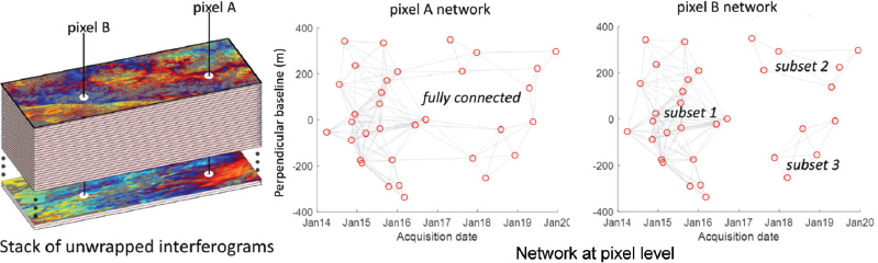
Figure 5.2. Two examples of networks at the pixel level starting from the network at the image level shown in Figure 5.1(b). The network of pixel A is fully connected despite some missing links with respect to the interferogram network at the image level (i.e. there are some interferograms in which pixel A is not unwrapped, but all dates are connected through a single network). The network of pixel B shows disconnected subsets due to missing links. In this case, recovering the full time series requires some assumptions and suitable inversion methods to reconnect the subsets. For a color version of this figure, see www.iste.co.uk/cavalie/images.zip
To tackle this problem, the small baseline subset (SBAS) technique uses a singular value decomposition (SVD) to solve the under-determined system (Berardino et al. 2002). More recently, several other implementations have been proposed to reconstruct the time series with different degrees of sophistication, including regularization constraints, the weighting of interferograms, solving for phase evolution and topographical residual error at the same time, the combination of information from low- and high-resolution interferograms through an iterative approach and correcting for unwrapping errors (Schmidt and Bürgmann 2003; Mora et al. 2003; Lanari et al. 2004; Fornaro et al. 2009; López-Quiroz et al. 2009; Doin et al. 2011; Jolivet et al. 2013; Yunjun et al. 2019). One of these implementations is discussed in more detail in section 5.4.
Compared to other methods such as PS or those that exploit all possible interferograms (see section 5.5), SBAS methods are confronted with the question of how to choose the optimal interferogram network. This choice is often based on empirical considerations about the quality of interferograms (with the difficulty that this may vary from region to region) and practical considerations about computational performance. This possible compromise makes SBAS methods competitive with respect to other methods, especially when very large areas (> millions of km2) need to be covered. To reach such coverage objectives, the problems of massive processing should also be taken into account (e.g. Casu et al. 2014; Manunta et al. 2019). Multi-looking is then commonly used to improve performance (e.g. Morishita et al. 2020). However, studies on phase closure, detailed in Chapter 6, have shown that this can lead to biases in the measurement of surface displacements, which must be taken into account.
5.3.2. From PS to PSDS
Permanent scatterer interferometry, developed in the late 1990s, is the first InSAR technique involving analysis directly from the measured wrapped phase in equation [5.4] (Ferretti et al. 2000, 2001). Parameters can be estimated through a search of the solution space, provided that the signal-to-noise ratio (SNR) is high enough. Consequently, the analysis is based only on selected pixels that are often characterized by highly coherent targets (i.e. low σ2noise), which typically correspond to human-made objects present over an urban city but which are less available in non-urban areas. Such stable targets, called permanent scatterers (Ferretti et al. 2000), have a dominant scatterer within the resolution cell and can be identified by a criterion relating to amplitude stability through time. Several approaches have been presented in previous studies for the performance of InSAR analysis over non-urban scenes (e.g. non-cultivated land, desert and debris areas) where the PS assumption cannot be retained by considering DS (Berardino et al. 2002; Lanari et al. 2004; Fialko 2006). In Figure 5.3, examples of PS and DS targets are shown.
The main aim is to achieve better performance by increasing the density of identified points by combining PS and DS targets. This combination has been proposed and studied by many authors (Fornaro et al. 2006; Rocca 2007; Ferretti et al. 2008, 2011; Hooper 2008). In Hooper (2008), a hybrid multi-temporal processing scheme was proposed, where two approaches (PS and SBAS) were applied to the same data input and then SBAS results were inverted by an SVD to be combined with PS. However, in the work of Fornaro et al. (2006), Ferretti et al. (2008), Ferretti et al. (2011) and Rocca (2007), the combination of PS and DS is carried out using a maximum likelihood (ML) estimation framework. In this approach, an optimized process for the parameters of interest can be implemented by exploiting target statistics, which can be represented by a coherence matrix. The advantage of this technique is that the criteria, which determine the weight of each interferogram in the estimation process, are directly derived from coherences through a rigorous mathematical approach. With the ML optimization, the parameters of interest can be asymptotically unbiased and of minimum variance. However, ML techniques require reliable information on target statistics (i.e. a coherence matrix) to determine the weight in the estimation algorithm.
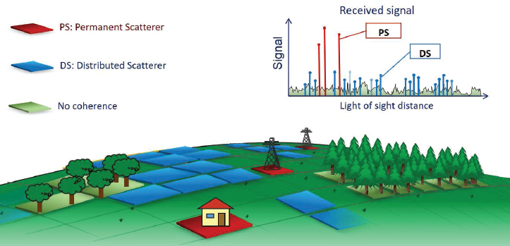
Figure 5.3. Examples of permanent and distributed scatterers. For a color version of this figure, see www.iste.co.uk/cavalie/images.zip
Rocca (2007) and Ferretti et al. (2011) have proposed a two-step ML estimation process. In the first step, the ML estimation is applied to all the N(N − 1)/2 interferograms available from N images, in order to squeeze the best estimates of the N − 1 interferometric phases, which is called SqueeSAR. This ML step was first known as phase linking (Guarnieri and Tebaldini 2008) or as the phase triangulation algorithm (PTA; Ferretti et al. 2011). This step is efficient and has a low computational burden. In the second step, the separation of the contributions of decorrelation noises from the parameters of interest can be processed as in the PS algorithm. Nowadays, the term “PSDS” refers to group techniques that exploit both PS and DS targets for time-series InSAR analysis.
5.4. The SBAS technique
5.4.1. Principle and definition of a “small baseline” network of interferograms
As shown in section 5.3, there is a continuum of methods from PS to small baseline subset techniques. Here, we focus on an end-member small baseline method that is determined by:
- – the definition of a “small baseline” network of interferograms;
- – multi-looking and spatial filtering of differential interferograms;
- – spatial unwrapping of spatially continuous interferograms after atmospheric and/or DEM error corrections;
- – time-series reconstruction of phase delay maps with time from a redundant network of interferograms;
- – source separation between atmospheric and deformation contributions.
While the exact order, combination and iteration of these steps depend on specific implementations, all of them are present in most SBAS algorithms. We here focus on the NSBAS chain organization of these steps (Doin et al. 2011), but we will mention some of the other SBAS chains. Note that the main difference with the PSDS technique, described above as an extension of the PS algorithms, is the assumption of a mostly continuous interferometric image sampled on a regular grid, as opposed to a discrete punctual sampling of space.
The basic rationale behind the SB technique is to recognize the non-closure behavior of the filtered unwrapped interferometric phase:
where A, B and C are three acquisitions and φAC, φAB, φBC are the unwrapped interferometric phases between A and C, A and B, and B and C, respectively (see Chapter 6). Non-closures are derived from three aspects: (a) range spectral filtering of the non-overlapping part of the spectrum between two single look complexes (SLCs) involved in the interferogram formation, (b) spatial averaging and filtering of complex values A1A2 exp(j(ϕ2 − ϕ1)) in the presence of decorrelation noise that reaches π, and (c) path-dependent unwrapping ambiguities.
Due to these three sources of non-closure, φAC brings complementary information to φAB and φBC. A key for the success of a particular SBAS implementation relies on how the information retrieval from each individual interferogram is maximized while minimizing the noise propagation, when the time series is reconstructed from a network of interferograms. For example, if A and C are taken during the same season, say autumn, while B is taken during spring, φAC might be more coherent than φAB + φBC, despite AB and BC being separated by a shorter time span than AC. In general, however, the longer the temporal or perpendicular baseline, the larger the phase noise in the full-resolution wrapped interferograms.
SB techniques thus try to optimize the choice of interferometric pairs by minimizing their perpendicular baseline, temporal baseline, seasonal difference, etc.
One source of decorrelation arises from the perpendicular baseline, which is mitigated by range spectral filtering. Range spectral filtering consists of removing the non-overlapping part of the range spectrum before interferogram computation. The relative apparent shift in the radar wavelength, as sensed by DSs on ground, between two acquisitions, depends on the terrain slope and the perpendicular baseline between two acquisitions (Gatelli et al. 1994). The overlapping fraction of the spectrum depends on the frequency shift and the range bandwidth. For ERS and Envisat data, for example, a perpendicular baseline of about 1,100 m leads to a complete disappearance of the spectrum overlap and thus a complete decorrelation of DSs. With adequate range spectrum filtering adapted to a local terrain slope (Davidson and Bamler 1999), interferograms with baselines up to 500 m can be obtained with a good preservation of the coherence over DSs. For ALOS interferograms, interferograms with very large perpendicular baselines can remain coherent due to a much larger range bandwidth than for ERS or Envisat. In the case of a restricted orbital tube and large bandwidth, such as Sentinel-1, the benefit of range spectral filtering is limited, and setting a small perpendicular baseline for interferograms is no longer the most critical criterion when defining the small baseline interferometric network.
A second source of decorrelation includes changes in land cover, soil moisture, etc. As time separation increases, the probability of the phase noise for each pixel going beyond π increases, either because of the complete change of a dominant scatterer or because of progressive transformation of multiple backscattering interactions within a resolution cell. As the phase is only known modulo 2π, a large phase noise produces a complete loss of information. Multi-looking and spatial filtering of small baseline interferograms are thus used to reduce phase noise before they are combined to reconstruct interferograms with any arbitrary temporal baseline. Therefore, SBAS methods can be considered as one way of solving for the ambiguity of phase noise in interferograms with large temporal baselines.
After multi-looking, filtering and unwrapping, the network of interferometric phases is inverted into time series. The temporal reconstruction consists of solving the overdetermined, but also possibly under-determined, set of equations:

where δφl are the unknown phase increments from acquisitions l to l+1 and φij is the kth unwrapped interferometric phase between date i and date j. If the above system is under-determined, or rank(GTG) < N − 1, with N being the number of images, it means that the interferometric network is made up of several (= N − rank(GTG)) independent subsets of images (Berardino et al. 2002; López-Quiroz et al. 2009). The relative information between independent subsets is missing. In order to reconstruct the time series, we must “invent” the missing links between subsets based on a predefined criterion. This additional criterion is the origin of the “subset” addition to the SBAS acronym. Although one may make an educated guess about the missing information (see, for example, López-Quiroz et al. (2009)), the disruption of the interferometric network into subsets will increase the uncertainty in the inverted time series, especially if subsets present no overlap in time.
To conclude, SBAS methods make it possible, using multi-looking and filtering of the interferometric phase in small baseline interferograms, to monitor the phase delay of a possibly evolving gathering of objects on the ground, with changing combinations of weights between backscatterers in the chosen neighborhood. To optimize the choice of the interferometric network, we must consider (1) a certain level of redundancy that will ensure a varied sampling of the above-mentioned combinations, (2) a perpendicular baseline that is small enough to preserve a spectrum overlap of at least half the range bandwidth, (3) a temporal baseline that enhances coherence and (4) network continuity from the first acquisition to the last one.
5.4.2. Multi-looking and filtering, atmospheric or DEM error corrections and unwrapping
As mentioned above, multi-looking and filtering are essential steps in SBAS techniques. Multi-looking is often performed on the complex interferogram, including the backscattering amplitude of the reference and secondary SLCs. As a result, high-intensity point scatterers, when present in the neighborhood, act as a huge weight on the multi-looked interferogram. Alternatively, in natural environments, the amplitude of the interferogram can be replaced by a measure of phase local stability, such as the collinearity defined by Pinel-Puyssegur et al. (2012), before multi-looking to increase the SNR of the multi-looked phase (Daout et al. 2018). There are many filtering methods (e.g. Goldstein and Werner 1998). Both multi-looking and filtering must preserve steep phase gradients, if there are any. When the latter occur along slopes in foreshortening areas, for example, or in incoherent areas, they produce inconsistencies in interferometric fringe patterns, which lead to unwrapping errors. This is why it is judicious to flatten the wrapped interferometric phase by, for example, correcting atmospheric delays and DEM errors before filtering and unwrapping (Doin et al. 2015; Daout et al. 2017; Maubant et al. 2020).
The component of the APS that can easily be corrected before filtering and unwrapping is the stratified atmospheric delay, i.e. the atmospheric contribution that is first-order dependent on elevation (see Chapter 4 and also Hanssen (2001) and Doin et al. (2009)). The stratified atmospheric correction can be evaluated empirically using the wrapped phase versus the elevation relationship (Grandin et al. 2012; Doin et al. 2015) or it can be predicted using global atmospheric models (Doin et al. 2009; Jolivet et al. 2011) together with GNSS zenith delays if present (Yu et al. 2018). In any case, it helps to reduce phase gradients in mountainous areas (Grandin et al. 2012) and thus facilitates filtering and unwrapping. The local DEM error correction can also be evaluated empirically using the relationship between the wrapped phase and the perpendicular baseline. This estimation can be performed for PSs or DSs (Ferretti et al. 2001; Hooper 2008) or for the whole multi-looked data stack (Ducret et al. 2014). It reduces the local phase scatter and again improves the multi-looking, filtering and unwrapping steps. Figure 5.4 shows the impact of corrections on wrapped interferograms, which can improve subsequent unwrapping.
When deformation gradients are very large and the deformation pattern is mostly constant through time, as in the case of subsidence in Mexico City (López-Quiroz et al. 2009) or permafrost dynamics Daout et al. (2017), it can be useful to obtain a preliminary deformation pattern map that can be scaled and removed before unwrapping and added back after unwrapping. Similarly, some authors prefer to remove a somewhat complex, empirically adjusted, stratified APS before unwrapping to efficiently remove steep phase gradients in mountainous areas, adding it back after unwrapping in order to make sure that there is no deformation leakage (Maubant et al. 2020). All this helps in solving unwrapping ambiguities that arise from abrupt phase gradients and/or from the presence of phase noise. The SBAS algorithm of Lanari et al. (2004) also presents an iterative unwrapping procedure where the first low-pass deformation time series obtained and the DEM correction map are used to correct wrapped interferograms and refine the unwrapping.
Finally, most of the SBAS methods rely on the spatial unwrapping of interferograms using different classes of methods (see Chapter 6): branch cut (Zebker and Lu 1998), global optimization (Chen and Zebker 2002) or spatial phase integration based on coherence (Grandin et al. 2012). The interferometric phase must be spatially continuous to connect all the parts of an interferogram without remaining 2π ambiguities. Spatial unwrapping is a critical step in InSAR processing, even for small baseline interferograms, especially in vegetated, mountainous or snowy regions. Note that in SBAS techniques this step replaces the spatial integration of velocity differences Δvpq and residual wrapped phase differences ![]() measured along the arcs pq of a network of PSDS points. The retrieved integrated residual phase, wn, of PSDSs for each time step n can also be affected by unwrapping errors due to possible large phase gradients related to the atmosphere (across atmospheric fronts or steep terrains) or nonlinear deformation between PSDS locations.
measured along the arcs pq of a network of PSDS points. The retrieved integrated residual phase, wn, of PSDSs for each time step n can also be affected by unwrapping errors due to possible large phase gradients related to the atmosphere (across atmospheric fronts or steep terrains) or nonlinear deformation between PSDS locations.
Once the interferograms have been unwrapped, they must be referenced by setting the average phase to zero in a given area. Unwrapped interferograms can also be flattened along the range, x, and azimuth, y, directions by adjusting a phase ramp in the form: ![]() In this case,
In this case, ![]() must be used to invert the time series
must be used to invert the time series ![]() for each time step l and then to reconstruct
for each time step l and then to reconstruct ![]() This ensures that the ramp correction is consistent within the interferogram network rule of thumb (Biggs et al. 2007). Alternatively, GPS data, within the InSAR footprint and converted to the LOS, can be used to fix the phase ramp.
This ensures that the ramp correction is consistent within the interferogram network rule of thumb (Biggs et al. 2007). Alternatively, GPS data, within the InSAR footprint and converted to the LOS, can be used to fix the phase ramp.
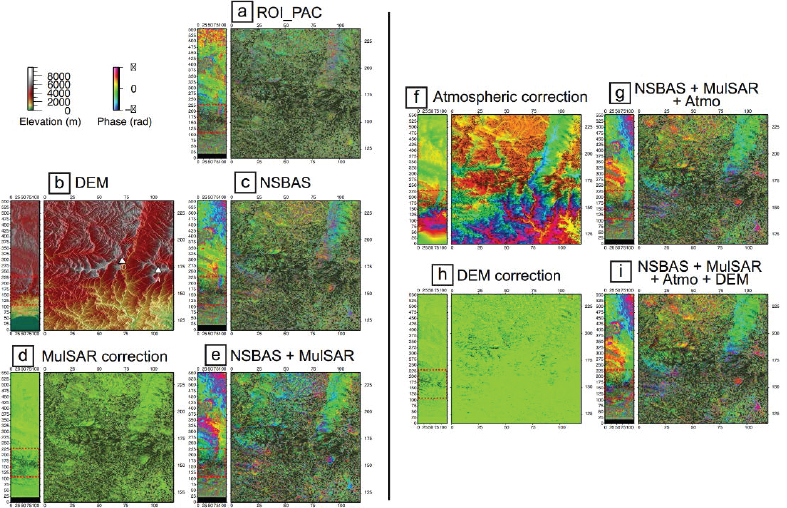
Figure 5.4. Examples showing how successive corrections on the wrapped phase help later unwrapping for a long temporal baseline Envisat interferogram (3.1 years) with a large perpendicular baseline (236 m) across the Himalayan range, i.e. in an area with strong relief and vegetation. The complete interferogram together with a zoom is shown at each correction step. The figure was reproduced from Grandin et al. (2012). (a) Multi-looked interferogram processed with ROI-PAC. (b) Shuttle Radar Topography Mission (SRTM) DEM in radar geometry. (c) Interferogram processed with NSBAS (Doin et al. 2011). (d) MulSAR correction (Pinel-Puyssegur et al. 2012). (e) Interferogram after the MulSAR correction. (f) Tropospheric delay correction computed from the ERA-Interim atmospheric model (Jolivet et al. 2011). (g) Interferogram after atmospheric correction. (h) DEM correction calculated from the combination of (wrapped) coherent interferograms with large perpendicular baselines and small temporal baselines (Ducret et al. 2014). (i) Interferogram after DEM correction. For a color version of this figure, see www.iste.co.uk/cavalie/images.zip
5.4.3. Reconstruction of the time series
We first focus here on the resolution of the set of equations [5.6], the only aim of which is to reconstruct the complete phase delay time series, including the residual atmospheric contribution. The linear system is written here for pedagogical purposes:
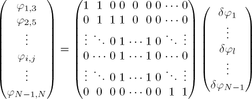
where φij are the M measured interferometric phases, N is the number of acquisitions and the M × (N − 1) matrix is the design matric G. It can be solved pixel by pixel by least squares or by singular value decomposition if the rank of GTG is lower than N − 1 (Berardino et al. 2002):
In order to determine how the data (φ) or model phase increments (δφinv) can be weighted by covariance matrices on the data Cd or on the model Cm in the estimation process, we must recall the reasons why the set of equations [5.6] will not be perfectly respected. The residuals φ − Gδφinv, in principle, contain only non-closure associated with multi-looking and filtering of phase decorrelation noise and unwrapping errors. Therefore, we can safely assume that there is no built-in covariance between the estimations of φAB, φBC and φAC, although they share common dates. The covariance, Cd, is thus to the first-order diagonal. Similarly, as the model phase increments contain two physical signals, deformation and atmospheric delay, there is no reason to include a temporal correlation length in the non-diagonal elements of Cm. Finally, we recommend a simple weighting of each equation in [5.6] by the amplitude of the estimated phase decorrelation noise, ![]() of each interferogram.
of each interferogram.
In the case of good data redundancy (evaluated by the data resolution matrix), and if unwrapping errors affect less than about one third of interferograms, the residuals between original and reconstructed interferograms, ![]() (with the interferogram ij corresponding to the kth interferogram), can be used to detect and correct unwrapping errors (Doin et al. 2011). We must first obtain rij by solving equation [5.7] and then by rule of thumb use these residuals to down-weight the set of equations by 1/(abs(rij) + r0), where r0 corresponds to a typical phase noise standard deviation, about 0.4 rad. Then, the residuals obtained with the new solution δφinv2 will point towards interferograms containing unwrapping errors. As a result, +/ − 2π can be added to the “wrong” φij values and a new solution can be computed. A few iterations allow us to converge to a consistent network of corrected unwrapped phases, provided that the number of initial errors affect only less than one fourth (by rule of thumb) the number of interferometric links.
(with the interferogram ij corresponding to the kth interferogram), can be used to detect and correct unwrapping errors (Doin et al. 2011). We must first obtain rij by solving equation [5.7] and then by rule of thumb use these residuals to down-weight the set of equations by 1/(abs(rij) + r0), where r0 corresponds to a typical phase noise standard deviation, about 0.4 rad. Then, the residuals obtained with the new solution δφinv2 will point towards interferograms containing unwrapping errors. As a result, +/ − 2π can be added to the “wrong” φij values and a new solution can be computed. A few iterations allow us to converge to a consistent network of corrected unwrapped phases, provided that the number of initial errors affect only less than one fourth (by rule of thumb) the number of interferometric links.
Finally, even if the built interferometric network does not isolate any image subsets, unwrapping may not have reached all the parts of interferograms, such that, for a given pixel, GTG might not be invertible. This is particularly common if there is snow during a part of the year, for example. In this case, singular value decomposition can be used, which will set the mean phase increment between the reconstructed phase through time of the different subsets to zero. However, this is not always the optimal way to reconstruct the missing information between subsets. Alternatively, we can implement constraints to provide the necessary interpolation across subsets using two equivalent approaches:
- – in the first, we compute the average velocity v, then subtract its contribution from each interferogram, φij − v × (tj − ti), and iterate on the time-series reconstruction. Afterwards, the offset between subsets obtained by SVD will correspond to the average velocity times the temporal separation of subsets. It is possible to write somewhat more complex formulations based on this principle;
- – in the second, we add constraints to the reconstructed phase with supplementary equations that model the phase behavior with time and/or the perpendicular baseline. The system then becomes invertible without having to resort to SVD.
In the following, we focus on the second case, i.e. the NSBAS inversion technique (Doin et al. 2011). The new constraints are applied in parallel to the first set of equations (equation [5.6]), meaning that we must solve additional variables, such as v, the acceleration a or a coefficient proportional to the perpendicular baseline B⊥, while still solving for the phase increments δφinv (López-Quiroz et al. 2009):
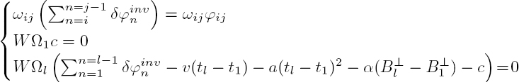
where tl and ![]() are the time and perpendicular baseline of acquisition l, respectively; l is greater than 2 in the last set of equations; and c is a constant. The weight W of the new constraint lines must be low enough for them not to affect the phase time-series reconstruction φlinv in the case of GTG being inversible. The weight ωij should depend on interferogram coherence: we can, for example, set it to be inversely proportional to the temporal baseline or, more empirically, inversely dependent on a measure of the local interferogram coherence. However, the weight Ωl should be set to be inversely correlated with the amplitude of the APS of each acquisition l. Therefore, the coefficients v, a, α and c are constrained mostly from acquisition dates with limited residual atmospheric contributions.
are the time and perpendicular baseline of acquisition l, respectively; l is greater than 2 in the last set of equations; and c is a constant. The weight W of the new constraint lines must be low enough for them not to affect the phase time-series reconstruction φlinv in the case of GTG being inversible. The weight ωij should depend on interferogram coherence: we can, for example, set it to be inversely proportional to the temporal baseline or, more empirically, inversely dependent on a measure of the local interferogram coherence. However, the weight Ωl should be set to be inversely correlated with the amplitude of the APS of each acquisition l. Therefore, the coefficients v, a, α and c are constrained mostly from acquisition dates with limited residual atmospheric contributions.
The deformation term may not be well represented by a linear term plus an acceleration. We can then decide to choose another parsimonious dictionary of functions, with a step (for earthquake), an exponential (for relaxation), trigonometric functions (for seasonal fluctuations), etc. Alternatively, for a very general inversion procedure, we can also decide to simultaneously invert for a smooth deformation contribution, with N additional variables, ![]() with l being the image acquisition (Doin et al. 2011):
with l being the image acquisition (Doin et al. 2011):
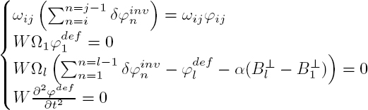
The constraint ![]() can be replaced by introducing a covariance between modeled variables
can be replaced by introducing a covariance between modeled variables ![]() through non-zero diagonal terms in Cm (Jolivet et al. 2013).
through non-zero diagonal terms in Cm (Jolivet et al. 2013).
Finally, for present-day SAR missions with systematic and massive acquisition strategies (such as Sentinel-1, every 6 or 12 days), resolving the above system of equations by progressive assimilation, as done by Dalaison and Jolivet (2020), strongly reduces the computational burden, while also making it possible to evaluate uncertainties.
Note that, in the NSBAS approach, in contrast to the traditional SBAS method (Lanari et al. 2004), the priors on ![]() are only used for regularization to fill the missing links, but the inverted phase time series
are only used for regularization to fill the missing links, but the inverted phase time series ![]() includes both the residual APS (after the correction of the stratified tropospheric effect) and the deformation, and it is not filtered in time. It can therefore be considered as a measurement with a quantified measurement error and it is obtained without an a priori constraint on deformation. This then makes it possible to proceed to geophysically driven source separation.
includes both the residual APS (after the correction of the stratified tropospheric effect) and the deformation, and it is not filtered in time. It can therefore be considered as a measurement with a quantified measurement error and it is obtained without an a priori constraint on deformation. This then makes it possible to proceed to geophysically driven source separation.
5.4.4. Source separation, atmosphere versus deformation
Source separation on the total phase delay time series (hereafter referred to as the “data cube”) should in principle allow us to (1) extract the deformation associated with different sources and discard the atmospheric phase screens and (2) quantify errors associated with this extraction. The source separation can be blind or aided by supplementary geophysical information. Blind methods allow us to explore datasets and prove the existence of a given geophysical signal, while geophysically aided extraction is more efficient for quantifying a giving process and giving an uncertainty in the result. In any case, adding a term proportional to the perpendicular baseline separates the residual contribution from the DEM error and helps in the retrieval of other geophysical signals.
The source separation problem can be solved with different approaches depending on the scientific goal. The “classical” blind method is to isolate APS by applying successive combinations of a high-pass filter to time followed by a low-pass filter to space for individual acquisitions (Berardino et al. 2002). The smoothed time series after the elimination of APS is the standard product given by many software packages, for example the P-SBAS approach (Lanari et al. 2020). However, possible leakages between APS and deformation, especially at large scales, cannot be easily evaluated using this approach. Furthermore, low-pass filtering a time series with uneven sampling, or sampled at a frequency lower than the oscillations of the signal, can produce strong aliasing (Doin et al. 2009). The phase delay data cube can also be explored using principal component analysis (Chaussard et al. 2014) or independent component analysis (ICA) (Ebmeier 2016; Maubant et al. 2020). The main contributions to the phase delay are then identified without introducing any external knowledge. For example, Maubant et al. (2020) could, using ICA, identify both the stratified atmospheric delay and the tenuous transient deformation signal, of a duration of a few months, associated with a slow slip event along the Pacific subduction zone in Mexico. In this case, the stratified APS showed a high-frequency component in time superimposed on a seasonal fluctuation, and, as a result, broke the basic assumption classically made for isolating APS. The validity of ICA source separation could then be checked using independent constraints from GNSS tropospheric and deformation measurements, as well as from the ERA-Interim atmospheric model from the European Centre for Median-Range Weather Forecasting (ECMWF).
Another type of approach involves seperating the sources using a regression analysis, assuming that deformation can be expressed by temporal functions (linear, seasonal, step, etc.). The advantages of this simple method are its robustness in the case of low SNR, the quantification of associated uncertainties and the possibility of weighting each acquisition based on the amplitude of its APS content. Note that retrieving only the LOS velocity field at the mm/yr accuracy is already a challenge at large scales. This is especially true when the expected deformation partly correlates with elevation, as is the case for some major faults (e.g. the Altyn Tagh fault (Elliott et al. 2008; Daout et al. 2018)) or volcanoes (Beauducel et al. 2000). Therefore, the uncertainty in the retrieved velocity field in mountainous areas cannot be discussed without a thorough error analysis of the stratified atmospheric correction. An in-depth presentation of how to derive the uncertainties in stratified atmospheric correction was proposed in Daout et al. (2018). Most regression analyses are performed on a pixel-by-pixel basis. However, Jolivet and Simons (2018) introduced a method that includes both spatial and temporal functions as well as a spatially correlated covariance matrix on the data.
Finally, source decomposition can be aided by modeling or a prior knowledge of the shape of the deformation in time, T (t), or in space, S(x, y). For example, assuming that the deformation associated with the load variation of the Siling Co lake is in the form T (t) ∗ S(x, y), a shape S(x, y) associated with known water level fluctuations can be retrieved or, inversely, the temporal behavior T (t) associated with the model shape of load-induced deflection can be estimated (Doin et al. 2015). The advantages again are the possibility of taking into account the noise properties of each acquisition and giving an error bar on T (t) or S(x, y). In addition, including modeling predictions for the east, north and up components, Mi(x, y), for different sources, i, also makes it possible to merge the time series obtained with different viewing angles using the unit LOS projection vector uLOS(x, y). This can be done by solving:
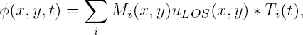
with possible regularization applied on Ti(t) (Grandin et al. 2010).
To conclude, the strength of the SBAS method is its ability to both adapt to the natural environment and provide a “data cube”, with the unwrapping error automatically being detected and corrected, including both deformation and residual atmospheric contributions and thus free from priors for the temporal or spatial behavior of deformation. Source separation adapted to the geophysical signal of interest can then be very efficient and accompanied by uncertainty estimates. In the following, we describe the PSDS method, which maximizes the retrieval of ground deformation from selected pixels or groups of neighboring pixels.
5.5. The PSDS technique
5.5.1. The PS algorithm
Let us now consider the phase difference between two neighboring PSs (e.g. targets p and q), which can be written as (Ferretti et al. 2000; Ho Tong Minh et al. 2020):
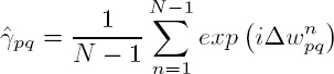
where W is the wrapping operator; Δεzpq is the relative elevation error between the targets p and q; Δvpq is the relative constant velocity; and ![]()
![]() is the difference between the observed and modeled phase for the points p and q in the n-th interferogram.
is the difference between the observed and modeled phase for the points p and q in the n-th interferogram.
The residue phase variance ![]() is the sum of three independent contributions,
is the sum of three independent contributions, ![]()
![]() Since a pair of neighboring PSs is not too far apart, low σ2aps (i.e. less than 0.1 rad2) can be expected for short distance (1 km) (Ferretti et al. 2000). In addition, the nonlinear motion of neighboring targets is highly correlated, resulting in a low
Since a pair of neighboring PSs is not too far apart, low σ2aps (i.e. less than 0.1 rad2) can be expected for short distance (1 km) (Ferretti et al. 2000). In addition, the nonlinear motion of neighboring targets is highly correlated, resulting in a low ![]() Finally, by definition, a low noise level is expected at the PS pixels. Thus,
Finally, by definition, a low noise level is expected at the PS pixels. Thus, ![]() remains low. In this case, it is possible to estimate Δεz and Δv by optimizing a figure of merit with a high degree of accuracy. In fact, Δεz and Δv can be jointly determined as the values that maximize the complex ensemble coherence in time
remains low. In this case, it is possible to estimate Δεz and Δv by optimizing a figure of merit with a high degree of accuracy. In fact, Δεz and Δv can be jointly determined as the values that maximize the complex ensemble coherence in time ![]() written as (Ferretti et al. 2000):
written as (Ferretti et al. 2000):
under the condition:
The absolute value of the coherence is in the range of 0 to 1. A value of 1 means a perfect match between the modeled phase and the observed phase. The ensemble coherence of PS pairs lower than a given threshold (e.g. 0.75) is usually discarded to maintain the high degree of accuracy.
In this way, ![]() can be calculated for every PS pair. Note that large distances (i.e. greater than 1 km) for a PS pair should be discarded to guarantee the conditions of equation [5.13]. Then, the variables εz and v can be calculated for PS targets by integrating their relative values,
can be calculated for every PS pair. Note that large distances (i.e. greater than 1 km) for a PS pair should be discarded to guarantee the conditions of equation [5.13]. Then, the variables εz and v can be calculated for PS targets by integrating their relative values, ![]() Most often, the computation is performed with respect to a reference pixel that is assumed to have known elevation and motion. By integrating the relative residual unwrapped phase difference
Most often, the computation is performed with respect to a reference pixel that is assumed to have known elevation and motion. By integrating the relative residual unwrapped phase difference ![]() from equation [5.11] over the whole network of PS pixels, we can obtain the unwrapped residual phase delays,
from equation [5.11] over the whole network of PS pixels, we can obtain the unwrapped residual phase delays, ![]() for each acquisition n and each PS p. Once the unwrapped phase of
for each acquisition n and each PS p. Once the unwrapped phase of ![]() is available, the atmospheric component can be separated by applying spatial–temporal filtering. After the atmospheric delays are estimated at the PS positions, a spatial interpolation can be applied to obtain the APS at the full resolution of differential interferograms.
is available, the atmospheric component can be separated by applying spatial–temporal filtering. After the atmospheric delays are estimated at the PS positions, a spatial interpolation can be applied to obtain the APS at the full resolution of differential interferograms.
5.5.2. PS selection
The main limitation of the PS approach outlined in section 5.5.1 lies in the sparsity of the grid for the selected PS. To overcome this limitation, the interpolated APSs are subtracted from differential interferograms, and additional PS candidates can be identified by applying a phase stability criterion. The computations described in section 5.5.1 are repeated for the new and denser PS network.
However, this PS technique has low performance in areas where the initial PS identification (i.e. based on the amplitude stability) does not suffice to cover the whole area of interest. This can occur for non-urban areas, especially for datasets suffering from amplitude calibration problems. The first solution to this problem was proposed by Hooper et al. (2004), who identified persistent scatterers based directly on the phase stability criterion rather than the amplitude stability. When compared to amplitude-based algorithms, this method has been shown to yield a denser point grid on rock areas. Nowadays, group techniques analyzing the time-series phase change of stable targets are referred to as persistent scatterer interferometry (PSI).
The gain performance of PSI is based on the selection of stable targets and their ability to remove the APS artifacts. The PSI technique offers a highly precise phase estimate despite temporal and geometrical decorrelations. Consequently, many related techniques have been investigated in the literature, for example interferometric point target analysis (Werner et al. 2003), coherent target monitoring (der Kooij 2003), the Stanford method for persistent scatterers (StaMPS) (Hooper et al. 2004), the spatial temporal unwrapping network (STUN) (Kampes 2006), persistent scatterer pairs (Costantini et al. 2008) and quasi-persistent scatterers (Perissin and Wang 2012). These techniques share similar properties in seeking modified approaches in order to improve the PS technique. The StaMPS algorithm makes no assumption of a prior deformation model and includes a three-dimensional phase unwrapping approach (Hooper and Zebker 2007; Hooper 2008). The STUN algorithm includes an integer least-squares estimator to solve equation [5.11] that allows us to drop the assumption made in equation [5.13]. Many methods have been proposed to add more reliable PS candidates (e.g. spectral phase diversity (Werner et al. 2003), a phase stability criterion (Hooper et al. 2004), maximum likelihood (Shanker and Zebker 2007)), resulting in a denser network and better estimation of phase measurements. The linear deformation model can be extended to consider thermal expansion (Monserrat et al. 2011) or to take into account seasonal motion phenomena (Colesanti et al. 2003). The signal model given in equation [5.1] makes an assumption of a dominant scatterer within the resolution cell. In practice, there could be more than one dominant point, as often is the case for layover due to buildings and towers. SAR tomography, which enables us to resolve layovers (Gini et al. 2002), can be exploited to relax this assumption. Siddique et al. (2016) demonstrated that the SAR tomography approach can improve deformation areas affected by layover.
The PSI method requires stable targets over a long time series. This results in a loss of information in some cases where stable points can be decorrelated in the majority of the low-coherence interferograms (Hooper et al. 2011). In such cases, the PS assumption can be relaxed by considering targets that are stable only in a subset of the dataset, for example temporary PSs (Ferrero et al. 2004; Hooper et al. 2011) and quasi-PSs (Perissin and Wang 2012). Finally, Ferretti et al. (2011) proposed an ML framework to consider both stable PS and slow decorrelation DS targets within the same PSI process. Hence, the PSDS algorithm is an extension of the PSI technique.
5.5.3. DS selection
DS targets are difficult to handle due to their low temporal coherence (Zebker and Villasenor 1992), which results in a low SNR. To enhance their SNRs, a number of pixels sharing the same statistical behavior can be exploited to make them emulate quasi-PSs. Groups of spatially close pixels that behave in a similar way (i.e. the same statistical behavior in the amplitude time series) must be identified. In practice, they can be selected by applying a two-sample Kolmogorov–Smirnov test (assuming a level of significance) to the amplitude time series of the considered pixel and all its neighbors. Pixels with a similar cumulative probability distribution are considered as “brothers”. Consequently, a brotherhood can be created, which results in a statistically homogeneous pixel (SHP) family. We can then compute the sample coherence matrix ![]() by taking advantage of the SHP family.
by taking advantage of the SHP family.
Decorrelating targets poses a challenge to time-series InSAR techniques. To overcome this challenge, ML estimation has been proposed to retrieve the linked phase time series (Rocca 2007; Guarnieri and Tebaldini 2008). As a result, the now commonly used PSDS technique outperforms PSI, particularly in non-urban areas (Ferretti et al. 2011). Consequently, this approach has become the main technique for surface deformation applications (Goel and Adam 2014; Ho Tong Minh et al. 2015, 2019; Cao et al. 2016; Cohen-Waeber et al. 2018).
Many approaches have been developed to improve the selection of the SHP family: the Anderson–Darling test (Goel and Adam 2014), fast statistically homogeneous pixel selection (Jiang et al. 2015), mean amplitude difference (Spaans and Hooper 2016), t-tests (Shamshiri et al. 2018) and similar time-series interferometric phase (Narayan et al. 2018) have been proposed to increase the number of DS points. These techniques aim to mitigate the bias in the sample coherence. A DS involves an assumption that there are independent small scatterers with a uniform scattering mechanism. This assumption can be relaxed by accounting for two or more scattering mechanisms (Cao et al. 2016; Engelbrecht and Inggs 2016). Engelbrecht and Inggs (2016) showed the enhancement of deformation measurements in agricultural areas when exploiting the multiple scattering mechanism approach with L-band ALOS PalSAR.
5.5.4. Phase linking
In SB approaches, signal decorrelations lead to the definition of interferogramswith short spatial and temporal baselines. With the ML estimation, all the N(N − 1)/2 interferograms available from N SLC images are jointly exploited in a complex coherence matrix. In fact, thanks to the redundancy of the phase differences between all given pairs, the phase can be improved by exploiting the consistency of phase closure of triplet information (i.e. the phases of a loop of three time instants I1-I2, I2-I3, I3-I1, which would be zero) (De Zan et al. 2015). The coherence matrix ![]() can fully characterize the target statistics and is used to invert for linked phases
can fully characterize the target statistics and is used to invert for linked phases ![]() as follows (Ferretti et al. 2011; Ho Tong Minh et al. 2020):
as follows (Ferretti et al. 2011; Ho Tong Minh et al. 2020):
where ![]() is the Hermitian conjugation; ◦ is the Hadamard entry-wise product;
is the Hermitian conjugation; ◦ is the Hadamard entry-wise product; ![]() is the estimated phase. It is noteworthy that the coherence matrix
is the estimated phase. It is noteworthy that the coherence matrix ![]() has an Hermitian symmetry that can be calculated using equation [4.12] for the SHP families. The estimated phase
has an Hermitian symmetry that can be calculated using equation [4.12] for the SHP families. The estimated phase ![]() quality can be assessed using PTA coherence, which can be defined as (Ferretti et al. 2011):
quality can be assessed using PTA coherence, which can be defined as (Ferretti et al. 2011):
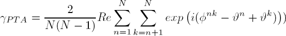
where φnk is the phase term corresponding to the off-diagonal elements of the coherence matrix ![]() If the γP T A coherence is above a certain threshold (e.g. 0.5), a DS point with the linked phase values
If the γP T A coherence is above a certain threshold (e.g. 0.5), a DS point with the linked phase values ![]() will be jointly processed with the PS using the PSI technique, as described in section 5.5.1.
will be jointly processed with the PS using the PSI technique, as described in section 5.5.1.
The linked phase is the key step in the PSDS technique, resulting in many studies focused on improving its performance. Cao et al. (2015) proposed equal-weighted and coherence-weighted approaches for phase estimation. Samiei-Esfahany et al. (2016) extended the PSI STUN algorithm (Kampes 2006; based on the least-squares principle for integer numbers) for slowly decorrelating targets. The component extraction and selection SAR (CAESAR) technique (Fornaro et al. 2015) can be exploited to decompose different scattering components from the coherence matrix (Cao et al. 2016). Ansari et al. (2017, 2018) proposed a sequential estimator for DS interferometry. Finally, Ho Tong Minh and Ngo (2021) introduced a compressed SAR (ComSAR) interferometric algorithm in the PSDS framework, particularly useful for matching in the analysis of big InSAR data.
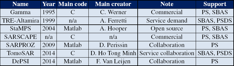
5.5.5. Tools supporting PS and PSDS processing
Today, a variety of software packages support PS processing, but there are only two PSDS tools available. The first package was developed by TRE-Altamira, who named it SqueeSAR (Ferretti et al. 2011). The TomoSAR platform created by D. Ho Tong Minh was originally developed at Politecnico di Milano, but subsequent development has taken place at the CESBIO and INRAE (Ho Tong Minh and Ngo 2017). Table 5.1 reports some well-known tools and their capabilities.
Although a Matlab license is required, the StaMPS code is the only open source tool available (Hooper et al. 2004). StaMPS can be used for PS or small baseline analysis. It allows the combination of PSs and DSs with a hybrid processing chain where two techniques (PS and SBAS) are applied, and then SBAS results are inverted by an SVD to be combined with PSs.
Table 5.1. Overview of PS and PSDS time-series software packages
Author contributions
Dinh Ho Tong Minh and Ramon Hanssen contributed to the sections on permanent/persistent scatterer and distributed scatterer InSAR techniques. Marie-Pierre Doin and Erwan Pathier contributed to the sections on small baseline methods. All authors read and approved the final manuscript.
5.6. Acknowledgments
We thank Fabio Rocca, Ekbal Hussain, Romain Jolivet and Raphaël Grandin for their constructive comments that improved the quality of this chapter.
5.7. References
Ansari, H., De Zan, F., Bamler, R. (2017). Sequential estimator: Toward efficient InSAR time series analysis. IEEE Transactions on Geoscience and Remote Sensing, 55(10), 5637–5652.
Ansari, H., De Zan, F., Bamler, R. (2018). Efficient phase estimation for interferogram stacks. IEEE Transactions on Geoscience and Remote Sensing, 56(7), 4109–4125.
Beauducel, F., Briole, P., Froger, J.-L. (2000). Volcano-wide fringes in ERS synthetic aperture radar interferograms of Etna (1992–1998): Deformation or tropospheric effect? Journal of Geophysical Research: Solid Earth, 105(B7), 16391–16402.
Berardino, P., Fornaro, G., Lanari, R., Sansosti, E. (2002). A new algorithm for surface deformation monitoring based on small baseline differential SAR interferograms. IEEE Transactions on Geoscience and Remote Sensing, 40(11), 2375–2383.
Biggs, J., Wright, T., Lu, Z., Parsons, B. (2007). Multi-interferogram method for measuring interseismic deformation: Denali Fault, Alaska. Geophysical Journal International, 170(3), 1165–1179.
Cao, N., Lee, H., Jung, H.C. (2015). Mathematical framework for phase-triangulation algorithms in distributed-scatterer interferometry. IEEE Geoscience and Remote Sensing Letters, 12(9), 1838–1842.
Cao, N., Lee, H., Jung, H.C. (2016). A phase-decomposition-based PSInSAR processing method. IEEE Transactions on Geoscience and Remote Sensing, 54(2), 1074–1090.
Casu, F., Elefante, S., Imperatore, P., Zinno, I., Manunta, M., De Luca, C., Lanari, R. (2014). SBAS-DInSAR parallel processing for deformation time-series computation. IEEE Journal of Selected Topics in Applied Earth Observations and Remote Sensing, 7(8), 3285–3296.
Chaussard, E., Bürgmann, R., Shirzaei, M., Fielding, E.J., Baker, B. (2014). Predictability of hydraulic head changes and characterization of aquifer-system and fault properties from InSAR-derived ground deformation. Journal of Geophysical Research: Solid Earth, 119(8), 6572–6590.
Chen, C.W. and Zebker, H.A. (2002). Phase unwrapping for large SAR interferograms: Statistical segmentation and generalized network models. IEEE Transactions on Geoscience and Remote Sensing, 40(8), 1709–1719.
Cohen-Waeber, J., Bürgmann, R., Chaussard, E., Giannico, C., Ferretti, A. (2018). Spatiotemporal patterns of precipitation-modulated landslide deformation from independent component analysis of InSAR time series. Geophysical Research Letters, 45(4), 1878–1887.
Colesanti, C., Ferretti, A., Novali, F., Prati, C., Rocca, F. (2003). SAR monitoring of progressive and seasonal ground deformation using the permanent scatterers technique. IEEE Transactions on Geoscience and Remote Sensing, 41(7), 1685–1701.
Costantini, M., Falco, S., Malvarosa, F., Minati, F. (2008). A new method for identification and analysis of persistent scatterers in series of SAR images. IEEE International Geoscience and Remote Sensing Symposium, 7–11 July.
Dalaison, M. and Jolivet, R. (2020). A Kalman filter time series analysis method for InSAR. Journal of Geophysical Research: Solid Earth, 125(7).
Daout, S., Doin, M.-P., Peltzer, G., Socquet, A., Lasserre, C. (2017). Large-scale InSAR monitoring of permafrost freeze-thaw cycles on the Tibetan Plateau. Geophysical Research Letters, 44(2), 901–909.
Daout, S., Doin, M.-P., Peltzer, G., Lasserre, C., Socquet, A., Volat, M., Sudhaus, H. (2018). Strain partitioning and present-day fault kinematics in NW Tibet from ENVISAT SAR interferometry. Journal of Geophysical Research: Solid Earth, 123(3), 2462–2483.
Davidson, G. and Bamler, R. (1999). Multiresolution phase unwrapping for SAR interferometry. IEEE Transactions on Geoscience and Remote Sensing, 37(1), 163–174.
De Zan, F., Zonno, M., Lopez-Dekker, P. (2015). Phase inconsistencies and multiple scattering in SAR interferometry. IEEE Transactions on Geoscience and Remote Sensing, 53(12), 6608–6616.
Doin, M.-P., Lasserre, C., Peltzer, G., Cavalié, O., Doubre, C. (2009). Corrections of stratified tropospheric delays in SAR interferometry: Validation with global atmospheric models. Journal of Applied Geophysics, 69(1), 35–50.
Doin, M.-P., Lodge, F., Guillaso, S., Jolivet, R., Lasserre, C., Ducret, G., Grandin, R., Pathier, E., Pinel, V. (2011). Presentation of the small baseline NSBAS processing chain on a case example: The Etna deformation monitoring from 2003 to 2010 using Envisat data. Fringe Workshop, Frascati.
Doin, M.-P., Twardzik, C., Ducret, G., Lasserre, C., Guillaso, S., Jianbao, S. (2015). InSAR measurement of the deformation around siling co lake: Inferences on the lower crust viscosity in central Tibet. Journal of Geophysical Research: Solid Earth, 2014JB011768.
Ducret, G., Doin, M.-P., Grandin, R., Lasserre, C., Guillaso, S. (2014). Dem corrections before unwrapping in a small baseline strategy for InSAR time series analysis. Geoscience and Remote Sensing Letters, 11(3), 696–700.
Ebmeier, S.K. (2016). Application of independent component analysis to multitemporal InSAR data with volcanic case studies. Journal of Geophysical Research: Solid Earth, 121(12), 8970–8986.
Elliott, J.R., Biggs, J., Parsons, B., Wright, T.J. (2008). InSAR slip rate determination on the Altyn Tagh Fault, northern Tibet, in the presence of topographically correlated atmospheric delays. Geophysical Research Letters, 35(12), L12309.
Emardson, T.R., Simons, M., Webb, F.H. (2003). Neutral atmospheric delay in interferometric synthetic aperture radar applications: Statistical description and mitigation. Journal of Geophysical Research, 108(B5), 2231.
Engelbrecht, J. and Inggs, M.R. (2016). Coherence optimization and its limitations for deformation monitoring in dynamic agricultural environments. IEEE Journal of Selected Topics in Applied Earth Observations and Remote Sensing, 9(12), 5647–5654.
Ferrero, A., Novali, F., Prati, C., Rocca, F. (2004). Advances in permanent scatterers analysis. Semi and temporary PS. European Conference on Synthetic Aperture Radar.
Ferretti, A., Prati, C., Rocca, F. (2000). Nonlinear subsidence rate estimation using permanent scatterers in differential SAR interferometry. IEEE Transactions on Geoscience and Remote Sensing, 38(5), 2202–2212.
Ferretti, A., Prati, C., Rocca, F. (2001). Permanent scatterers in SAR interferometry. IEEE Transactions on Geoscience and Remote Sensing, 39(1), 8–20.
Ferretti, A., Novali, F., De Zan, F., Prati, C., Rocca, F. (2008). Moving from PS to slowly decorrelating targets: A prospective view. European Conference on Synthetic Aperture Radar, 2–5 June.
Ferretti, A., Fumagalli, A., Novali, F., Prati, C., Rocca, F., Rucci, A. (2011). A new algorithm for processing interferometric data-stacks: SqueeSAR. IEEE Transactions on Geoscience and Remote Sensing, 49(9), 3460–3470.
Fialko, Y. (2006). Interseismic strain accumulation and the earthquake potential on the southern San Andreas fault system. Nature, 441, 968–971.
Fornaro, G., Monti Guarnieri, A., Pauciullo, A., De Zan, F. (2006). Maximum liklehood multi-baseline SAR interferometry. IEE Proceedings – Radar, Sonar and Navigation, 153(3), 279–288.
Fornaro, G., Pauciullo, A., Serafino, F. (2009). Deformation monitoring over large areas with multipass differential SAR interferometry: A new approach based on the use of spatial differences. International Journal of Remote Sensing, 30(6), 1455–1478.
Fornaro, G., Verde, S., Reale, D., Pauciullo, A. (2015). CAESAR: An approach based on covariance matrix decomposition to improve multibaseline–multitemporal interferometric SAR processing. IEEE Transactions on Geoscience and Remote Sensing, 53(4), 2050–2065.
Gatelli, F., Guamieri, A.M., Parizzi, F., Pasquali, P., Prati, C., Rocca, F. (1994). The wavenumber shift in SAR interferometry. IEEE Transactions on Geoscience and Remote Sensing, 32(4), 855–865.
Ghiglia, D.C. and Pritt, M.D. (1998). Two-Dimensional Phase Unwrapping: Theory, Algorithms, and Software. John Wiley & Sons, Inc., New York.
Gini, F., Lombardini, F., Montanari, M. (2002). Layover solution in multibaseline SAR interferometry. IEEE Transactions on Aerospace and Electronic Systems, 38(4), 1344–1356.
Goel, K. and Adam, N. (2014). A distributed scatterer interferometry approach for precision monitoring of known surface deformation phenomena. IEEE Transactions on Geoscience and Remote Sensing, 52(9), 5454–5468.
Goldstein, R.M. and Werner, C.L. (1998). Radar interferogram filtering for geophysical applications. Geophysical Research Letters, 25(21), 2517–2520.
Grandin, R., Socquet, A., Doin, M.-P., Jacques, E., de Chabalier, J.-B., King, G.C.P. (2010). Transient rift opening in response to multiple dike injections in the Manda Hararo rift (Afar, Ethiopia) imaged by time-dependent elastic inversion of interferometric synthetic aperture radar data. Journal of Geophysical Research: Solid Earth, 115(B9), B09403.
Grandin, R., Doin, M.-P., Bollinger, L., Pinel-Puysségur, B., Ducret, G., Jolivet, R., Sapkota, S.N. (2012). Long-term growth of the Himalaya inferred from interseismic InSAR measurement. Geology, 40(12), 1059–1062.
Guarnieri, A.M. and Tebaldini, S. (2008). On the exploitation of target statistics for SAR interferometry applications. IEEE Transactions on Geoscience and Remote Sensing, 46(11), 3436–3443.
Hanssen, R.F. (2001). Radar Interferometry: Data Interpretation and Error Analysis. Kluwer Academic Publishers, Dordrecht.
Ho Tong Minh, D. and Ngo, Y.-N. (2017). Tomosar platform supports for Sentinel-1 tops persistent scatterers interferometry. IEEE International Geoscience and Remote Sensing Symposium (IGARSS), 1680–1683.
Ho Tong Minh, D. and Ngo, Y.-N. (2021). ComSAR: A new algorithm for processing big data SAR interferometry. IEEE International Geoscience and Remote Sensing Symposium (IGARSS), 1–4.
Ho Tong Minh, D., Van Trung, L., Toan, T.L. (2015). Mapping ground subsidence phenomena in Ho Chi Minh City through the radar interferometry technique using ALOS PALSAR data. Remote Sensing, 7(7), 8543–8562.
Ho Tong Minh, D., Tran, Q.C., Pham, Q.N., Dang, T.T., Nguyen, D.A., El-Moussawi, I., Le Toan, T. (2019). Measuring ground subsidence in Ha Noi through the radar interferometry technique using TerraSAR-X and Cosmos SkyMed data. IEEE Journal of Selected Topics in Applied Earth Observations and Remote Sensing, 12(10), 3874–3884.
Ho Tong Minh, D., Hanssen, R., Rocca, F. (2020). Radar interferometry: 20 years of development in time series techniques and future perspectives. Remote Sensing, 12(9), 1364.
Hooper, A. (2008). A multi-temporal InSAR method incorporating both persistent scatterer and small baseline approaches. Geophysical Research Letters, 35(L16302), 1–5.
Hooper, A. and Zebker, H.A. (2007). Phase unwrapping in three dimensions with application to InSAR time series. JOSA A, 24(9), 2737–2747.
Hooper, A., Zebker, H.A., Segall, P., Kampes, B. (2004). A new method for measuring deformation on volcanoes and other natural terrains using InSAR persistent scatterers. Geophysical Research Letters, 31(23), L23611.
Hooper, A., Ofeigsson, B., Sigmundsson, F. (2011). Increased capture of magma in the crust promoted by ice-cap retreat in Iceland. Nature Geoscience, 4, 783–786.
Jiang, M., Ding, X., Hanssen, R.F., Malhotra, R., Chang, L. (2015). Fast statistically homogeneous pixel selection for covariance matrix estimation for multitemporal InSAR. IEEE Transactions on Geoscience and Remote Sensing, 53(3), 1213–1224.
Jolivet, R. and Simons, M. (2018). A multipixel time series analysis method accounting for ground motion, atmospheric noise, and orbital errors. Geophysical Research Letters, 45(4), 1814–1824.
Jolivet, R., Grandin, R., Lasserre, C., Doin, M.-P., Peltzer, G. (2011). Systematic InSAR tropospheric phase delay corrections from global meteorological reanalysis data. Geophysical Research Letters, 38(17), L17311.
Jolivet, R., Lasserre, C., Doin, M.-P., Peltzer, G., Avouac, J.-P., Sun, J., Dailu, R. (2013). Spatio-temporal evolution of aseismic slip along the Haiyuan Fault, China: Implications for fault frictional properties. Earth and Planetary Science Letters, 377–378, 23–33.
Kampes, B. (2006). Radar Interferometry: Persistent Scatterer Technique. Springer Publishing Company, New York.
der Kooij, V. (2003). Coherent target analysis. Fringe Workshop, Frascati.
Lanari, R., Mora, O., Manunta, M., Mallorqui, J.J., Berardino, P., Sansosti, E. (2004). A small-baseline approach for investigating deformations on full-resolution differential SAR interferograms. IEEE Transactions on Geoscience and Remote Sensing, 42(7), 1377–1386.
Lanari, R., Bonano, M., Casu, F., Luca, C.D., Manunta, M., Manzo, M., Onorato, G., Zinno, I. (2020). Automatic generation of Sentinel-1 continental scale DInSAR deformation time series through an extended P-SBAS processing pipeline in a cloud computing environment. Remote Sensing, 12(18), 2961.
López-Quiroz, P., Doin, M.-P., Tupin, F., Briole, P., Nicolas, J.-M. (2009). Time series analysis of Mexico City subsidence constrained by radar interferometry. Journal of Applied Geophysics, 69(1), 1–15.
Manunta, M., De Luca, C., Zinno, I., Casu, F., Manzo, M., Bonano, M., Fusco, A., Pepe, A., Onorato, G., Berardino, P., De Martino, P., Lanari, R. (2019). The parallel SBAS approach for Sentinel-1 interferometric wide swath deformation time-series generation: Algorithm description and products quality assessment. IEEE Transactions on Geoscience and Remote Sensing, 57(9), 6259–6281.
Maubant, L., Pathier, E., Daout, S., Radiguet, M., Doin, M.-P., Kazachkina, E., Kostoglodov, V., Cotte, N., Walpersdorf, A. (2020). Independent component analysis and parametric approach for source separation in InSAR time series at regional scale: Application to the 2017–2018 slow slip event in Guerrero (Mexico). Journal of Geophysical Research: Solid Earth, 125(3), e2019JB018187.
Monserrat, O., Crosetto, M., Cuevas, M., Crippa, B. (2011). The thermal expansion component of persistent scatterer interferometry observations. IEEE Geoscience and Remote Sensing Letters, 8(5), 864–868.
Mora, O., Mallorqui, J.J., Broquetas, A. (2003). Linear and nonlinear terrain deformation maps from a reduced set of interferometric SAR images. IEEE Transactions on Geoscience and Remote Sensing, 41(10), 2243–2253.
Morishita, Y., Lazecky, M., Wright, T.J., Weiss, J.R., Elliott, J.R., Hooper, A. (2020). LiCSBAS: An open-source InSAR time series analysis package integrated with the LiCSAR automated Sentinel-1 InSAR processor. Remote Sensing, 12(3), 424.
Narayan, A.B., Tiwari, A., Dwivedi, R., Dikshit, O. (2018). A novel measure for categorization and optimal phase history retrieval of distributed scatterers for InSAR applications. IEEE Transactions on Geoscience and Remote Sensing, 56(10), 5843–5849.
Perissin, D. and Wang, T. (2012). Repeat-pass SAR interferometry with partially coherent targets. IEEE Transactions on Geoscience and Remote Sensing, 50(1), 271–280.
Pinel-Puyssegur, B., Michel, R., Avouac, J.-P. (2012). Multi-link InSAR time series: Enhancement of a wrapped interferometric database. IEEE Journal of Selected Topics in Applied Earth Observations and Remote Sensing, 5(3), 784–794.
Rocca, F. (2007). Modeling interferogram stacks. IEEE Transactions on Geoscience and Remote Sensing, 45(10), 3289–3299.
Samiei-Esfahany, S., Martins, J.E., van Leijen, F., Hanssen, R.F. (2016). Phase estimation for distributed scatterers in InSAR stacks using integer least squares estimation. IEEE Transactions on Geoscience and Remote Sensing, 54(10), 5671–5687.
Schmidt, D.A. and Bürgmann, R. (2003). Time-dependent land uplift and subsidence in the Santa Clara valley, California, from a large interferometric synthetic aperture radar data set. Journal of Geophysical Research, 108(B9), 2416.
Shamshiri, R., Nahavandchi, H., Motagh, M., Hooper, A. (2018). Efficient ground surface displacement monitoring using Sentinel-1 data: Integrating distributed scatterers (DS) identified using two-sample t-test with persistent scatterers (PS). Remote Sensing, 10(5), 794.
Shanker, P. and Zebker, H.A. (2007). Persistent scatterer selection using maximum likelihood estimation. Geophysical Research Letters, 34(22), L22301.
Siddique, M.A., Wegmüller, U., Hajnsek, I., Frey, O. (2016). Single-look SAR tomography as an add-on to PSI for improved deformation analysis in urban areas. IEEE Transactions on Geoscience and Remote Sensing, 54(10), 6119–6137.
Spaans, K. and Hooper, A. (2016). InSAR processing for volcano monitoring and other near-real time applications. Journal of Geophysical Research: Solid Earth, 121(4), 2947–2960.
Usai, S., Del Gaudio, C., Borgstrom, S., Achilli, V. (1999). Monitoring terrain deformations at Phlegrean Fields with SAR interferometry. Fringe 99 Workshop, Liège.
Werner, C., Wegmuller, U., Strozzi, T., Wiesmann, A. (2003). Interferometric point target analysis for deformation mapping. IEEE International Geoscience and Remote Sensing Symposium, 7, 4362–4364
Wright, T.J., Parsons, B., Fielding, E. (2001). Measurement of interseismic strain accumulation across the North Anatolian Fault by satellite radar interferometry. Geophysical Research Letters, 28(10), 2117–2120.
Yu, C., Li, Z., Penna, N.T., Crippa, P. (2018). Generic atmospheric correction model for interferometric synthetic aperture radar observations. Journal of Geophysical Research: Solid Earth, 123(10), 9202–9222.
Yunjun, Z., Fattahi, H., Amelung, F. (2019). Small baseline InSAR time series analysis: Unwrapping error correction and noise reduction. Computers and Geosciences, 133, 104331.
Zebker, H.A. and Lu, Y. (1998). Phase unwrapping algorithms for radar interferometry: Residue-cut, least-squares, and synthesis algorithms. Journal of the Optical Society of America A, 15(3), 586–598.
Zebker, H.A. and Villasenor, J. (1992). Decorrelation in interferometric radar echoes. IEEE Transactions on Geoscience and Remote Sensing, 30(5), 950–959.