Chapter Four. Geometry for Modeling and Design
Objectives
After studying the material in this chapter, you should be able to:
1. Identify and specify basic geometric elements and primitive shapes.
2. Select a 2D profile that best describes the shape of an object.
3. Identify mirrored shapes and sketch their lines of symmetry.
4. Identify shapes that can be formed by extrusion and sketch their cross sections.
5. Identify shapes that can be formed by revolution techniques and sketch their profiles.
6. Define Boolean operations.
7. Specify the Boolean operations to combine primitive shapes into a complex shape.
8. Work with Cartesian coordinates and user coordinate systems in a CAD system.
9. Identify the transformations common to CAD systems.
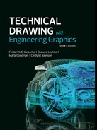
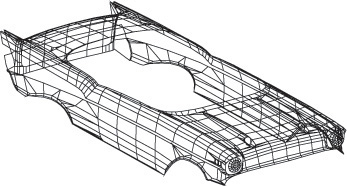
Many different geometric shapes were used to model this jetboard. The wireframe view of the top cover reveals several regular geometric shapes used to model the interior components. The graceful lines of the outer hull are defined by the irregular curves used to model it. (Courtesy of Leo Greene, www.e-Cognition.net.)
Coordinates for 3D CAD Modeling
2D and 3D CAD drawing entities are stored in relationship to a Cartesian coordinate system. No matter what CAD software system you will be using, it is helpful to understand some basic similarities of coordinate systems.
Most CAD systems use the right-hand rule for coordinate systems; if you point the thumb of your right hand in the positive direction for the X-axis and your index finger in the positive direction for the Y-axis, your remaining fingers will curl in the positive direction for the Z-axis (shown in Figure 4.1). When the face of your monitor is the X-Y plane, the Z-axis is pointing toward you (see Figure 4.2).


4.2 The Z-Axis. In systems that use the right-hand rule, the positive Z-axis points toward you when the face of the monitor is parallel to the X-Y plane.
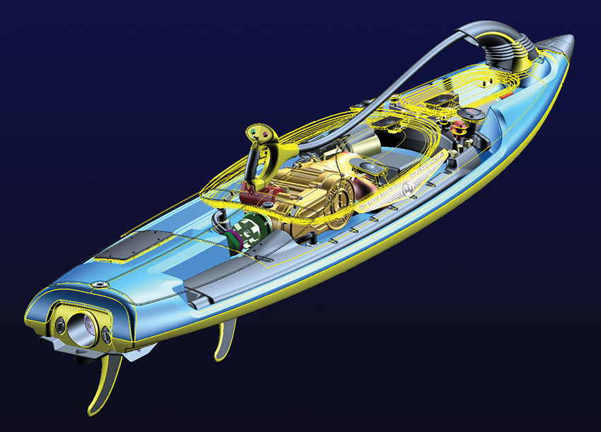
The right-hand rule is also used to determine the direction of rotation. For rotation using the right-hand rule, point your thumb in the positive direction along the axis of rotation. Your fingers will curl in the positive direction for the rotation, as shown in Figure 4.3.
4.3 Axis of Rotation. The curl of the fingers indicates the positive direction along the axis of rotation.
Though rare, some CAD systems use a left-hand rule. In this case, the curl of the fingers on your left hand gives you the positive direction for the Z-axis. In this case, when the face of your computer monitor is the X-Y plane, the positive direction for the Z-axis extends into your computer monitor, not toward you.
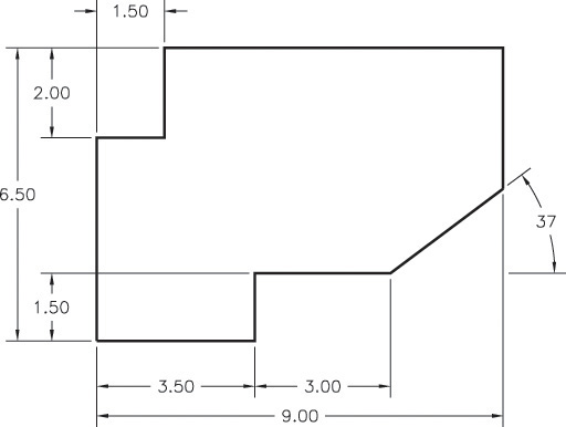
A 2D CAD system uses only the X- and Y-coordinates of the Cartesian coordinate system. 3D CAD systems use X, Y, and Z. To represent 2D in a 3D CAD system, the view is straight down the Z-axis. Figure 4.4 shows a drawing created using only the X- and Y- values, leaving the Z-coordinates set to 0, to produce a 2D drawing.

4.4 2D CAD Drawing. This drawing was created on the X-Y plane in the CAD system. It appears true shape because the viewing direction is perpendicular to the X-Y plane—straight down the Z-axis.
Recall that each orthographic view shows only two of the three coordinate directions because the view is straight down one axis. 2D CAD drawings are the same: They show only the X- and Y-coordinates because you are looking straight down the Z-axis.
When the X-Y plane is aligned with the screen in a CAD system, the Z-axis is oriented horizontally. In machining and many other applications, the Z-axis is considered to be the vertical axis. In all cases, the coordinate axes are mutually perpendicular and oriented according to the right-hand or left-hand rule. Because the view can be rotated to be straight down any axis or any other direction, understanding how to use coordinates in the model is more important than visualizing the direction of the default axes and planes.
The vertices of the 3D shape shown in Figure 4.5 are identified by their X-, Y-, and Z-coordinates. Often, it is useful when modeling parts to locate the origin of the coordinate system at the lower left of the part, as shown in Figure 4.5. This location for the (0,0,0) point on a part is useful when the part is being machined, as it then makes all coordinates on the part positive (Figure 4.6). Some older numerically-controlled machinery will not interpret a file correctly if it has negative lengths or coordinates. CAD models are often exported to other systems for manufacturing parts, so try to create them in a common and useful way.

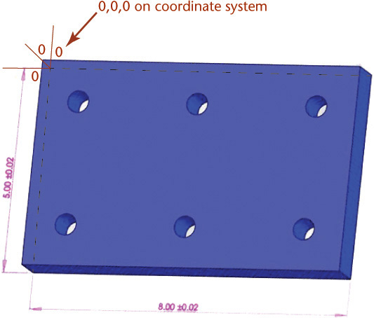
4.6 This CAD model for a plate with 6 holes has its origin (0,0,0) at the back left of the part when it is set up for numerically-controlled machining. (Courtesy of Matt McCune, Autopilot, Inc.)
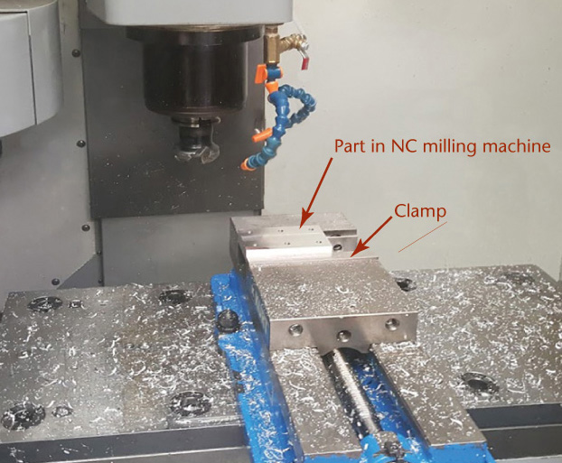
4.7 The part is clamped in place during machining. The back left corner of the part is the 0,0,0 location during the machining process. (Courtesy of Matt McCune, Autopilot, Inc.)
Specifying Location
Even though the model is ultimately stored in a single Cartesian coordinate system, you may usually specify the location of features using other location methods as well. The most typical of these are relative, polar, cylindrical, and spherical coordinates. These coordinate formats are useful for specifying locations to define your CAD drawing geometry.
Absolute Coordinates
Absolute coordinates are used to store the locations of points in a CAD database. These coordinates specify location in terms of distance from the origin in each of the three axis directions of the Cartesian coordinate system.
Think of giving someone directions to your house (or to a house in an area where the streets are laid out in rectangular blocks). One way to describe how to get to your house would be to tell the person how many blocks over and how many blocks up it is from two main streets (and how many floors up in the building, for 3D). The two main streets are like the X- and Y-axes of the Cartesian coordinate system, with the intersection as the origin. Figure 4.8 shows how you might locate a house with this type of absolute coordinate system.
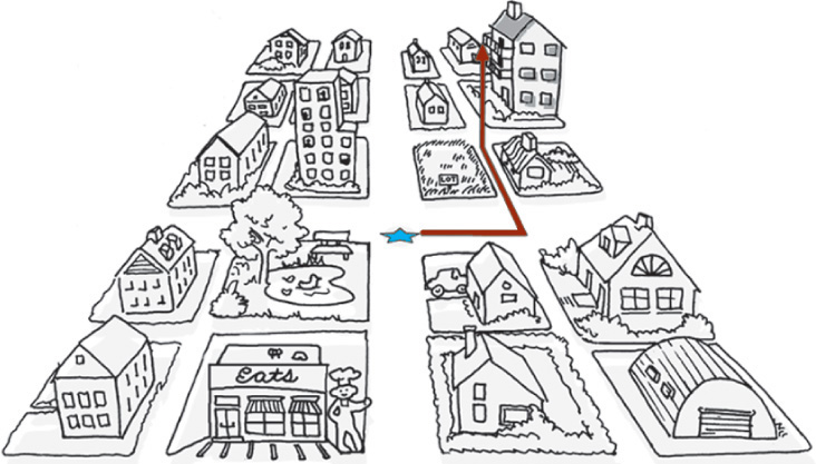
4.8 Absolute coordinates define a location in terms of distance from the origin (0,0,0), shown here as a star. These directions are useful because they do not change unless the origin changes.
Relative Coordinates
Instead of having to specify each location from the origin, you can use relative coordinates to specify a location by giving the number of units from a previous location. In other words, the location is defined relative to your previous location.
To understand relative coordinates, think about giving someone directions from his or her current position, not from two main streets. Figure 4.9 shows the same map again, but this time with the location of the house relative to the location of the person receiving directions.
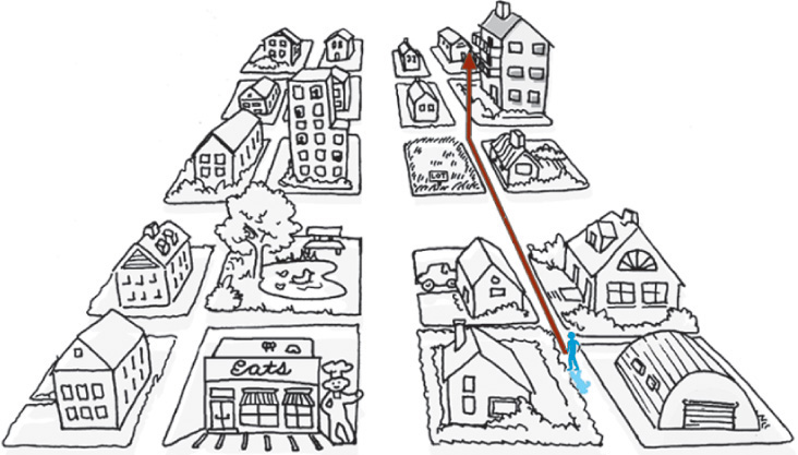
4.9 Relative coordinates describe the location in terms of distance from a starting point. Relative coordinates to the same location differ according to the starting location.
Polar Coordinates
Polar coordinates are used to locate an object by giving an angle (from the X-axis) and a distance. Polar coordinates can either be absolute, giving the angle and distance from the origin, or relative, giving the angle and distance from the current location.
Picture the same situation of having to give directions. You could tell the person to walk at a specified angle from the crossing of the two main streets, and how far to walk. Figure 4.10 shows the angle and direction for the shortcut across the empty lot using absolute polar coordinates. You could also give directions as an angle and distance relative to a starting point.

4.10 Polar coordinates describe the location using an angle and distance from the origin (absolute) or starting point (relative).
Cylindrical and Spherical Coordinates
Cylindrical and spherical coordinates are similar to polar coordinates except that a 3D location is specified instead of one on a single flat plane (such as a map).
Cylindrical coordinates specify a 3D location based on a radius, angle, and distance (usually in the Z-axis direction). This gives a location as though it were on the edge of a cylinder. The radius tells how far the point is from the center (or origin); the angle is the angle from the X-axis along which the point is located; and the distance provides the height where the point is located on the cylinder. Cylindrical coordinates are similar to polar coordinates, but they add distance in the Z-direction. Figure 4.11a depicts relative cylindrical coordinates used to specify a location, where the starting point serves as the center of the cylinder.

4.11 Relative Cylindrical and Spherical Coordinates. The target points in (a) and (b) are described by relative coordinates from the starting point (3,2,0). Although the paths to the point differ, the resulting endpoint is the same.
Spherical coordinates specify a 3D location by the radius, an angle from the X-axis, and the angle from the X-Y plane. These coordinates locate a point on a sphere, where the origin of the coordinate system is at the center of the sphere. The radius gives the size of the sphere; the angle from the X-axis locates a place on the equator. The second angle gives the location from the plane of the equator to a point on the sphere in line with the location specified on the equator. Figure 4.11b depicts relative spherical coordinates, where the starting point serves as the center of the sphere.
Even though you may use these different systems to enter information into your 3D drawings, the end result is stored using one set of Cartesian coordinates.
Using Existing Geometry to Specify Location
Most CAD packages offer a means of specifying location by specifying a the relationship of a point to existing objects in the model or drawing. For example, AutoCAD’s “object snap” feature lets you enter a location by “snapping” to the endpoint of a line, the center of a circle, the intersection of two lines, and so on (Figure 4.12). Using existing geometry to locate new entities is faster than entering coordinates. This feature also allows you to capture geometric relationships between objects without calculating the exact location of a point. For example, you can snap to the midpoint of a line or the nearest point of tangency on a circle. The software calculates the exact location.

4.12 Object snaps are aids for selecting locations on existing CAD drawing geometry. (Autodesk screen shots reprinted courtesy of Autodesk, Inc.)
Geometric Entities
Points
Points are geometric constructs. Points are considered to have no width, height, or depth. They are used to indicate locations in space. In CAD drawings, a point is located by its coordinates and usually shown with some sort of marker like a cross, circle, or other representation. Many CAD systems allow you to choose the style and size of the mark that is used to represent points.
Most CAD systems offer three ways to specify a point:
• Type in the coordinates (of any kind) for the point (see Figure 4.13).

4.13 Specifying Points. Point 1 was added to the drawing by typing the absolute coordinates 3,4,7. Point 2 was added relative to Point 1 with the relative coordinates @2,2,2.
• Pick a point from the screen with a pointing device (mouse or tablet).
• Specify the location of a point by its relationship to existing geometry (e.g., an endpoint of a line, an intersection of two lines, or a center point).
Picking a point from the screen is a quick way to enter points when the exact location is not important, but the accuracy of the CAD database makes it impossible to enter a location accurately in this way.
Lines
A straight line is defined as the shortest distance between two points. Geometrically, a line has length but no other dimension such as width or thickness. Lines are used in drawings to represent the edge view of a surface, the limiting element of a contoured surface, or the edge formed where two surfaces on an object join. In a CAD database, lines are typically stored by the coordinates of their endpoints.
For the lines shown in Figure 4.14, the table below shows how you can specify the second endpoint for a particular type of coordinate entry. (For either or both endpoints, you can also snap to existing geometry without entering any coordinates.)
|
(a) Second Endpoint for 2D Line |
(b) Second Endpoint |
Absolute |
6,6 |
5,4,6 |
Relative |
@3,4 |
@2,2,6 |
Relative polar |
@5<53.13 |
n/a |
Relative cylindrical |
n/a |
@2.8284<45,6 |
Relative spherical |
n/a |
@6.6332<45<64.7606 |

4.14 Specifying Lines. (a) This 2D line was drawn from endpoint (3,2) to (6,6). (b) This 3D line was drawn from endpoint (3,2,0) to (5,4,6).
Planes
Planes are defined by any of the following (see Figure 4.15):
• Three points not lying in a straight line
• Two parallel lines
• Two intersecting lines
• A point and a line
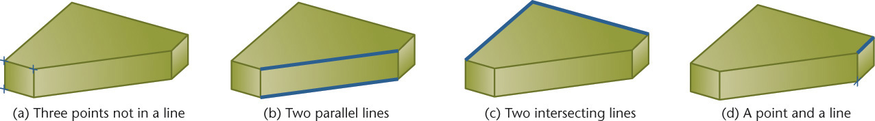
The last three ways to define a plane are all special cases of the more general case—three points not in a straight line. Knowing what can determine a plane can help you understand the geometry of solid objects and use the geometry as you model in CAD.
For example, a face on an object is a plane that extends between the vertices and edges of the surface. Most CAD programs allow you to align new entities with an existing plane. You can use any face on the object—whether it is normal, inclined, or oblique—to define a plane for aligning a new entity.
Defining planes on the object or in 3D space is an important skill for working in 3D CAD. The software provides tools for defining new planes (see Figure 4.16). The options for these tools are based on the geometry of planes, as defined in the preceding list. Typical choices allow the use of any three points not in a line, two parallel lines, two intersecting lines, a point and a line, or being parallel to, perpendicular to, or at an angle from an existing plane.
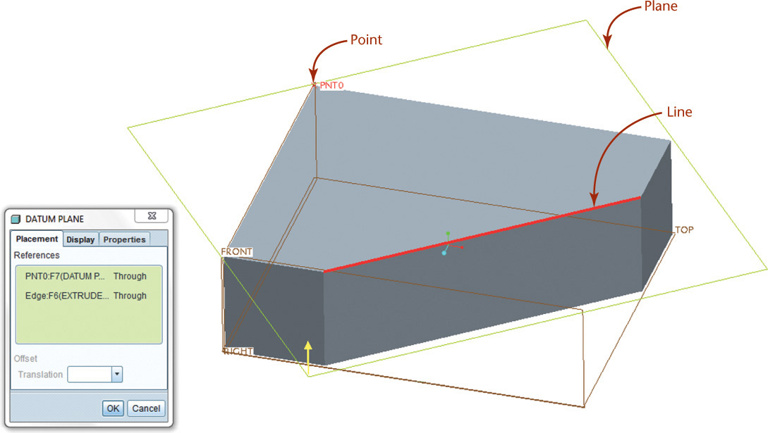
4.16 Defining a Plane in CAD. A point and a line (the edge between two surfaces in this case) were used to define a plane in this Pro/ENGINEER model.
A plane may serve as a coordinate-system orientation that shows a surface true shape. You will learn more about orienting work planes to take advantage of the object’s geometry later in this chapter.
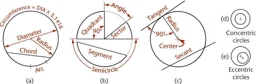
Circles
A circle is a set of points that are equidistant from a center point. The distance from the center to one of the points is the radius (see Figure 4.17). The distance across the center to any two points on opposite sides is the diameter. The circumference of a circle contains 360° of arc. In a CAD file, a circle is often stored as a center point and a radius.
4.18 AutoCAD Circle Construction Options (Autodesk screen shots reprinted courtesy of Autodesk, Inc.)
Spotlight: Formulas for Circles and Arcs
r = radius
C = circumference
π = pi ≅ 3.14159
a = arc length
A = area
L = chord length
θ (theta) = included angle
rad (radian) = the included angle of an arc length such that the arc length is equal to the radius
C = 2πr, the curved distance around a circle
A = πr2, the area of a circle
a = 2πr × θ/360, so the arc length = 0.01745rθ when you know its radius, r, and the included angle, θ, in degrees
a = r × θ (when the included angle is measured in radians)

Bolt-Hole Circle Chord Lengths
To determine the distance between centers for equally spaced holes on a bolt-hole circle:
n = 180/number of holes in pattern
L = sin n × bolt-hole circle diameter
EXAMPLE: 8-hole pattern on a 10.00-diameter circle:
180/8 = 22.5
sin of 22.5 is .383
.383 × 10 = 3.83 (chord length)
For more useful formulas, see Appendix 3.

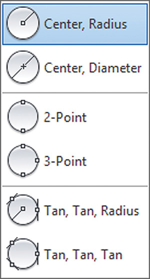
Most CAD systems allow you to define a circle by specifying any one of the following:
• the center and a diameter
• the center and a radius
• two points on the diameter
• three points on the circle
• a radius and two entities to which the circle is tangent
• three entities to which the circle is tangent.
These methods are illustrated in Figure 4.19.

Arcs
An arc is a portion of a circle. An arc can be defined by specifying any one of the following (see Figure 4.20):
• a center, radius, and angle measure (sometimes called the included angle or delta angle)
• a center, radius, and chord length
• a center, radius, and arc length
• the endpoints and a radius
• the endpoints and a chord length
• the endpoints and arc length
• the endpoints and one other point on the arc (3 points)
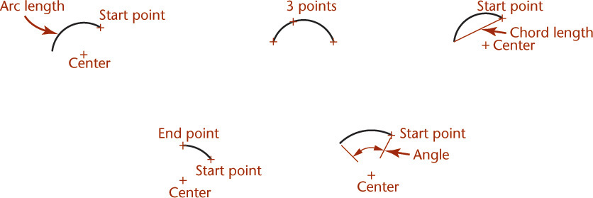
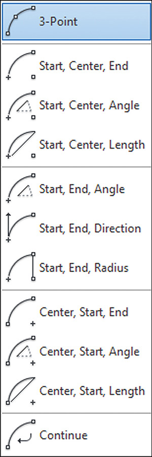
4.20 Defining Arcs. Arcs can be defined many different ways. Like circles, arcs may be located from a center point or an endpoint, making it easy to locate them relative to other entities in the model.
4.1 Manually Bisecting a Line or Circular Arc
Figure 4.22a shows the given line or arc AB to be bisected.
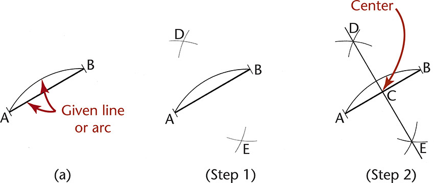
Step 1. From A and B draw equal arcs with their centers at the endpoints and a with radius greater than half AB.
Step 2. Join intersections D and E with a straight line to locate center C.
Tip: Accurate Geometry with AutoCAD
Using object snaps (Figure A) to locate drawing geometry, such as the midpoint of the arc shown in Figure B, is a quick and easy way to draw a line bisecting an arc or another line.

(A) The AutoCAD Drafting Settings dialog box can be used to turn on objects snaps, a method of selecting locations on drawing geometry. (Autodesk screen shots reprinted courtesy of Autodesk Inc.)

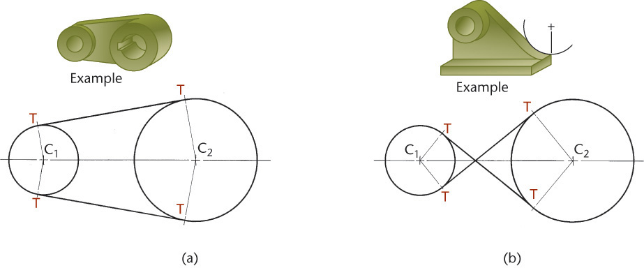
4.2 Drawing Tangents to Two Circles
When drawing entities tangent to a circle, there are two locations that satisfy the condition of tangency. When using a CAD system, select a point close to the tangent location you intend.

4.3 Drawing an Arc Tangent to a Line or Arc and Through a Point
Given line AB, point P, and radius R (Figure 4.25a), draw line DE parallel to the given line and distance R from it. From P draw an arc with radius R, cutting line DE at C, the center of the required tangent arc.
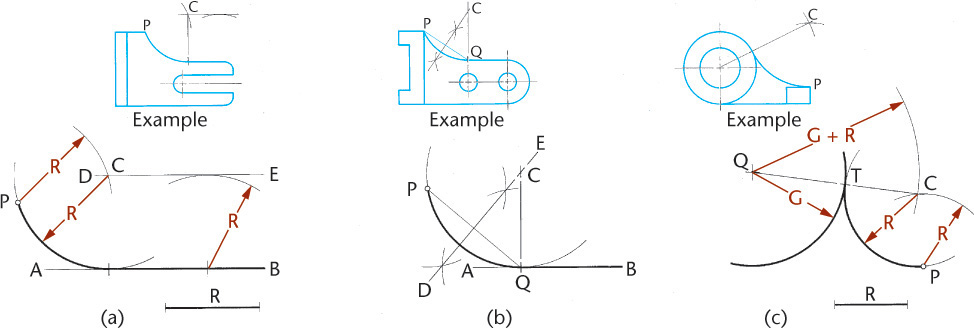
Given line AB, with tangent point Q on the line and point P (Figure 4.25b), draw PQ, which will be a chord of the required arc. Draw perpendicular bisector DE, and at Q draw a line perpendicular to the line to intersect DE at C, the center of the required tangent arc.
Given an arc with center Q, point P, and radius R (Figure 4.25c), from P, draw an arc with radius R. From Q, draw an arc with radius equal to that of the given arc plus R. The intersection C of the arcs is the center of the required tangent arc.
Step by Step: Drawing an Arc Tangent to Two Arcs
Creating Construction Geometry
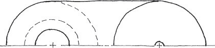
CAD software typically provides a command option to draw a circle or arc tangent to two entities (any combination of arcs, circles, or lines) given the radius. For example, the AutoCAD Circle command has an option called Ttr (tangent, tangent, radius). When you use this command, you first select the two drawing objects to which the new circle will be tangent and then enter the radius.
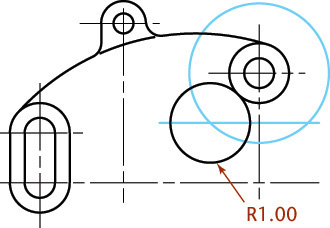
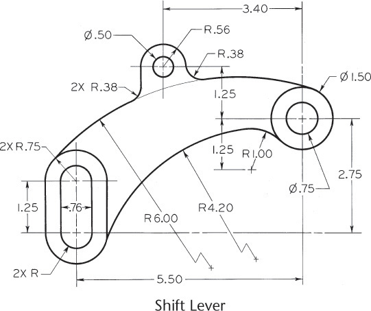
Take a look at the shift lever drawing. To draw this figure you must use a geometric construction to find the center of the 1.00-radius tangent arc. Before the lower 4.20-radius arc can be drawn, the smaller 1.00-radius arc must be constructed tangent to the 1.50 diameter circle. When an arc is tangent to a circle, its center must be the radius distance away from that circle.
![]() Use basic CAD commands to draw the portions shown.
Use basic CAD commands to draw the portions shown.

![]() Construct circle B with a radius 1.00 larger than circle A. You can use the AutoCAD Offset command to do this quickly. The desired tangent arc must have its center somewhere on circle B. The vertical dimension of 1.25 is given between the two centers in the drawing. Construct line C at this distance. The only point that is on both the circle and the line is the center of the desired tangent arc.
Construct circle B with a radius 1.00 larger than circle A. You can use the AutoCAD Offset command to do this quickly. The desired tangent arc must have its center somewhere on circle B. The vertical dimension of 1.25 is given between the two centers in the drawing. Construct line C at this distance. The only point that is on both the circle and the line is the center of the desired tangent arc.

![]() Draw the 1.00-radius circle tangent to the 1.50-diameter circle and centered on the point just found.
Draw the 1.00-radius circle tangent to the 1.50-diameter circle and centered on the point just found.
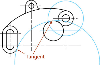
![]() Next, construct the lower arc to be tangent to the lower curve at the left of the 1.00-radius circle. Then, trim the circles at their intersections to form the desired arcs.
Next, construct the lower arc to be tangent to the lower curve at the left of the 1.00-radius circle. Then, trim the circles at their intersections to form the desired arcs.
Geometric Constraints
Using geometric constraints is another way to create this CAD geometry. When geometric constraints are used, a general-case arc can be drawn that is not perfectly tangent. Then, a tangent constraint, the vertical dimension between the arc center and the circle, and the required radius can be applied to the arc as drawn. The software will then calculate the correct arc based on these constraints.
If the desired distance changes, the dimensional constraint values can be updated, and the software will recalculate the new arc. Not all software provides constraint-based modeling, especially in a 2D drafting context. The AutoCAD software has had this feature since release 2010.
When using constraint-based modeling, you still must understand the drawing geometry clearly to create a consistent set of geometric and dimensional constraints.
Tip
Two different tangent circles with the same radius are possible—one as shown and one that includes both circles. To get the desired arc using AutoCAD, select near the tangent location for the correctly positioned arc.
4.4 Bisecting an Angle
Figure 4.26a shows the given angle BAC to be bisected.

Step 1. Lightly draw large arc with center at A to intersect lines AC and AB.
Step 2. Lightly draw equal arcs r with radius slightly larger than half BC, to intersect at D.
Step 3. Draw line AD, which bisects the angle.
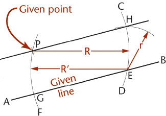
4.5 Drawing a Line through a Point and Parallel to a Line
With given point P as center, and any convenient radius R, draw arc CD to intersect the given line AB at E (Figure 4.27). With E as center and the same radius, strike arc R′ to intersect the given line at G. With PG as radius and E as center, strike arc r to locate point H. The line PH is the required parallel line.
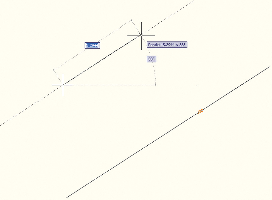
Using AutoCAD, you can quickly draw a new line parallel to a given line and through a given point using the Offset command with the Through option. Another method is to use the Parallel object snap while drawing the line as shown in Figure 4.28. You can also copy the original line and place the copy through the point.
4.6 Drawing a Triangle with Sides Given
Given the sides A, B, and C, as shown in Figure 4.29a,
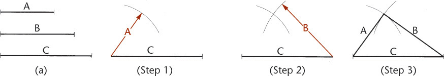
Step 1. Draw one side, as C, in the desired position, and draw an arc with radius equal to side A.
Step 2. Lightly draw an arc with radius equal to side B.
Step 3. Draw sides A and B from the intersection of the arcs, as shown.
Tip
Using AutoCAD, you can enter the relative length and angle from the previous endpoint using the format: @lengthvalue<anglevalue
4.7 Drawing a Right Triangle with Hypotenuse and One Side Given
Given sides S and R (Figure 4.30), with AB as a diameter equal to S, draw a semicircle. With A as center and R as radius, draw an arc intersecting the semicircle at C. Draw AC and CB to complete the right triangle.

4.8 Laying Out an Angle
Many angles can be laid out directly with the triangle or protractor. For more accuracy, use one of the methods shown in Figure 4.31.

Tangent Method The tangent of angle θ is y/x, and y = x tan θ. Use a convenient value for x, preferably 10 units (Figure 4.31a). (The larger the unit, the more accurate will be the construction.) Look up the tangent of angle θ and multiply by 10, and measure y = 10 tan θ.
EXAMPLE To set off 31-1/2°, find the natural tangent of 31-1/2°, which is 0.6128. Then, y = 10 units × 0.6128 = 6.128 units.
Sine Method Draw line x to any convenient length, preferably 10 units (Figure 4.31b). Find the sine of angle θ, multiply by 10, and draw arc with radius R = 10 sin θ. Draw the other side of the angle tangent to the arc, as shown.
EXAMPLE To set off 25-1/2°, find the natural sine of 25-1/2°, which is 0.4305. Then R = 10 units × 0.4305 = 4.305 units.
Chord Method Draw line x of any convenient length, and draw an arc with any convenient radius R—say 10 units (Figure 4.31c). Find the chordal length C using the formula C = 2 sin θ/2. Machinists’ handbooks have chord tables. These tables are made using a radius of 1 unit, so it is easy to scale by multiplying the table values by the actual radius used.
EXAMPLE Half of 43°20′ = 21°40′. The sine of 21°40′ = 0.3692. C = 2 × 0.3692 = 0.7384 for a 1 unit radius. For a 10 unit radius, C = 7.384 units.
EXAMPLE To set off 43°20′, the chordal length C for 1 unit radius, as given in a table of chords, equals 0.7384. If R = 10 units, then C = 7.384 units.
4.9 Drawing an Equilateral Triangle
Side AB is given. With A and B as centers and AB as radius, lightly construct arcs to intersect at C (Figure 4.32a). Draw lines AC and BC to complete the triangle.

Alternative Method Draw lines through points A and B, making angles of 60° with the given line and intersecting C (Figure 4.32b).
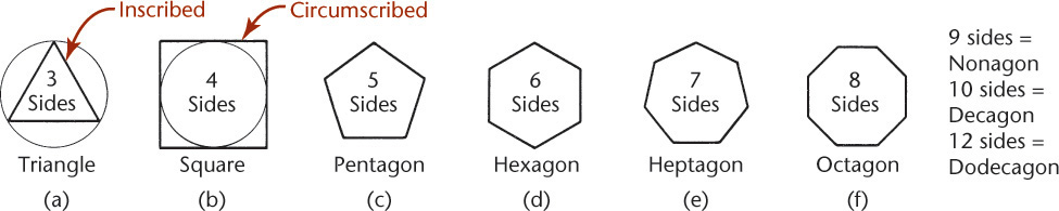
4.10 Polygons
A polygon is any plane figure bounded by straight lines (Figure 4.33). If the polygon has equal angles and equal sides, it can be inscribed in or circumscribed around a circle and is called a regular polygon.
Tip
The AutoCAD Polygon command is used to draw regular polygons with any number of sides. The polygon can be based on the radius of an inscribed or circumscribed circle. The length of an edge of the polygon can also be used to define the size. Figure 4.34 shows the quick help for the Polygon command. The Rectangle command is another quick way to make a square in AutoCAD.

4.34 Polygons can be defined by the number of sides and whether they are inscribed or circumscribed in a circle. (Autodesk screen shots reprinted courtesy of Autodesk, Inc.)
4.11 Drawing a Regular Pentagon
Dividers Method: Divide the circumference of the circumscribed circle into five equal parts with the dividers, and join the points with straight lines (Figure 4.35a).

Geometric Method:
Step 1. Bisect radius OD at C (Figure 4.35b).
Step 2. Use C as the center and CA as the radius to lightly draw arc AE. With A as center and AE as radius, draw arc EB (Figure 4.35c).
Step 3. Draw line AB, then measure off distances AB around the circumference of the circle. Draw the sides of the pentagon through these points (Figure 4.35d).
4.12 Drawing a Hexagon
Each side of a hexagon is equal to the radius of the circumscribed circle (Figure 4.36a). To use a compass or dividers, use the radius of the circle to mark the six points of the hexagon around the circle. Connect the points with straight lines. Check your accuracy by making sure the opposite sides of the hexagon are parallel.

Centerline Variation Draw vertical and horizontal centerlines (Figure 4.36b). With A and B as centers and radius equal to that of the circle, draw arcs to intersect the circle at C, D, E, and F, and complete the hexagon as shown.
Hexagons, especially when drawn to create bolt heads, are usually dimensioned by the distance across the flat sides (not across the corners). When creating a hexagon using CAD, it is typical to draw it as circumscribed about a circle, so that the circle diameter is defining the distance across the flat sides of the hexagon (see Figure 4.32).

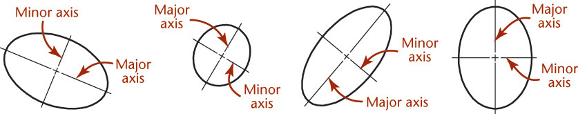
4.13 Ellipses
An ellipse can be defined by its major and minor axis distances. The major axis is the longer axis of the ellipse; the minor axis is the shorter axis. Some ellipses are shown and labeled in Figure 4.38.
An ellipse is created by a point moving along a path where the sum of its distances from two points, each called a focus of an ellipse (foci is the plural form), is equal to the major diameter. As an aid in understanding the shape of an ellipse, imagine pinning the ends of a string in the locations of the foci, then sliding a pencil along inside the string, keeping it tightly stretched, as in Figure 4.39. You would not use this technique when sketching, but it serves as a good illustration of the definition of an ellipse.
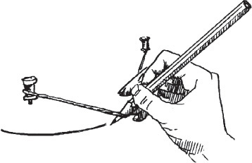
4.39 Pencil and String Method. When an ellipse is created with the pencil-and-string method, the length of the string between the foci is equal to the length of the major axis of the ellipse. Any point that can be reached by a pencil inside the string when it is pulled taut meets the condition that its distances from the two foci sum to the length of the major diameter.
Most CAD systems provide an Ellipse command that lets you enter the major and minor axis lengths, center, or the angle of rotation for a circle that is to appear elliptical.
Spotlight: Locating the Foci of an Ellipse
To locate the foci of an ellipse, draw arcs with their centers at the ends of the minor axis and their radii equal to half the major axis. The intersection of each pair of arcs is a focus of the ellipse.

Spotlight: The Perimeter of an Ellipse
The perimeter, P, of an ellipse is a set of points defined by their distance from the two foci. The sum of the distances from any point on the ellipse to the two foci must be equal to the length of the major diameter. The perimeter of an ellipse may be approximated in different ways. Many CAD packages use infinite series to most closely approximate the perimeter. The mathematical relationship of each point on the ellipse to the major and minor axes may be seen in the approximation of the perimeter at right:

4.14 Spline Curves
Splines are used to describe complex, or freeform, curves. Many surfaces cannot be easily defined using simple curves such as circles, arcs, or ellipses. For example, the flowing curves used in automobile design blend many different curves into a smooth surface. Creating lifelike shapes and aerodynamic forms may require spline curves (Figure 4.40).
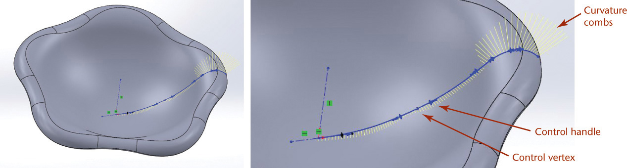
4.40 Complex Curves. The organic shape of this flowerlike bowl was created using SolidWorks splines. Splines can be controlled in a variety of ways. The enlarged view shows the curvature combs used to view the effect of the controlling curves that make up the spline. Dragging a control handle changes the direction of the curve at the control vertex. (Courtesy of Robert Kincaid.)
The word spline originally described a flexible piece of plastic or rubber used to draw irregular curves between points. Mathematical methods generate the points on the curve for CAD applications.
One way to create an irregular curve is to draw curves between each set of points. The points and the tangencies at each point are used in a polynomial equation that determines the shape of the curve. This type of curve is useful in the design of a ship’s hull or an aircraft wing. Because this kind of irregular curve passes through all the points used to define the curve, it is sometimes called an interpolated spline or a cubic spline. An example and its vertices are shown in Figure 4.41.
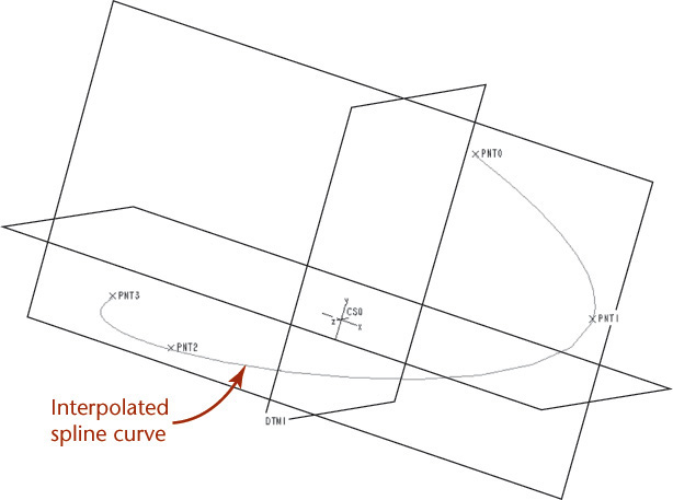
4.41 Interpolated Spline. An interpolated spline curve passes through all the points used to define the curve.
Other spline curves are approximated: they are defined by a set of vertices. The resulting curve does not pass through all the vertices. Instead, the vertices “pull” the curve in the direction of the vertex. Complex curves can be created with relatively few vertices using approximation methods. Figure 4.42 shows a 3D approximated spline curve and its vertices.
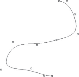
4.42 Approximated Spline. Except for the beginning and endpoints, the fit points for the spline curve stored in the database do not always lie on the curve. They are used to derive the curve mathematically.
The mathematical definition for this type of spline curve uses the X- and Y- (and Z- for a 3D shape) coordinates and a parameter, generally referred to as u. A polynomial equation is used to generate functions in u for each point used to specify the curve. The resulting functions are then blended to generate a curve that is influenced by each point specified but not necessarily coincident with any of them.
The Bezier curve was one of the first methods to use spline approximation to create flowing curves in CAD applications. The first and last vertices are on the curve, but the rest of the vertices contribute to a blended curve between them. The Bezier method uses a polynomial curve to approximate the shape of a polygon formed by the specified vertices. The order of the polynomial is 1 degree less than the number of vertices in the polygon (see Figure 4.43).

4.43 Bezier Curve. A Bezier curve passes through the first and last vertex but uses the other vertices as control points to generate a blended curve.
The Bezier method is named for Pierre Bezier, a pioneer in computer-generated surface modeling at Renault, the French automobile manufacturer. Bezier sought an easier way of controlling complex curves, such as those defined in automobile surfaces. His technique allowed designers to shape natural-looking curves more easily than they could by specifying points that had to lie on the resulting curve, yet the technique also provided control over the shape of the curve. Changing the slope of each line segment defined by a set of vertices adjusts the slope of the resulting curve (see Figure 4.44). One disadvantage of the Bezier formula is that the polynomial curve is defined by the combined influence of every vertex: a change to any vertex redraws the entire curve between the start point and endpoint.

4.44 Editing a Bezier Curve. Every vertex contributes to the shape of a Bezier curve. Changing the location of a single vertex redraws the entire curve.
A B-spline approximation is a special case of the Bezier curve that is more commonly used in engineering to give the designer more control when editing the curve. A B-spline is a blended piecewise polynomial curve passing near a set of control points. The spline is referred to as piecewise because the blending functions used to combine the polynomial curves can vary over the different segments of the curve. Thus, when a control point changes, only the piece of the curve defined by the new point and the vertices near it change, not the whole curve (see Figure 4.45). B-splines may or may not pass through the first and last points in the vertex set. Another difference is that for the B-spline the order of the polynomial can be set independently of the number of vertices or control points defining the curve.

4.45 B-Spline Approximation. The B-spline is constructed piecewise, so changing a vertex affects the shape of the curve near only that vertex and its neighbors.
In addition to being able to locally modify the curve, many modelers allow sets of vertices to be weighted differently. The weighting, sometimes called tolerance, determines how closely the curve should fit the set of vertices. Curves can range from fitting all the points to being loosely controlled by the vertices. This type of curve is called a nonuniform rational B-spline, or NURBS curve. A rational curve (or surface) is one that has a weight associated with each control point.
Splines are drawn in CAD systems based on the mathematical relationships defining their geometry. Figure 4.46 shows an approximated spline drawn using AutoCAD. Figure 4.47 shows an interpolated spline drawn using SolidWorks. Both curves are drawn with a spline command, and both provide a dialog box that allows you to change properties defining the curve; however, the properties that are controlled vary by the type of spline being created by the software package. You should be familiar with the terms used by your modeling software for creating different types of spline curves.

4.46 Approximated Spline. This spline drawn in AutoCAD is pulled toward the defined control points. The Properties dialog box at the right allows you to change the weighting factor for each control point. (Autodesk screen shots reprinted courtesy of Autodesk, Inc.)
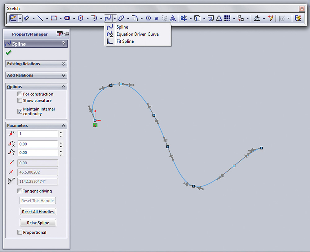
4.47 Interpolated Spline. This SolidWorks spline passes through each control point. Software tools allow you to control spline properties. (Image courtesy of ©2016 Dassault Systèmes SolidWorks Corporation.)
4.15 Geometric Relationships
When you are sketching, you often imply a relationship, such as being parallel or perpendicular, by the appearance of the lines or through notes or dimensions. When you are creating a CAD model you use drawing aids to specify these relationships between geometric entities.
Two lines or planes are parallel when they are an equal distance apart at every point. Parallel entities never intersect, even if extended to infinity. Figure 4.48 shows an example of parallel lines.
Two lines or planes are perpendicular when they intersect at right angles (or when the intersection that would be formed if they were extended would be a right angle), as in Figure 4.49.
Two entities intersect if they have at least one point in common. Two straight lines intersect at only a single point. A circle and a straight line intersect at two points, as shown in Figure 4.50.

When two lines intersect, they define an angle as shown in Figure 4.51.
4.51 An angle is defined by the space between two lines (such as those highlighted here) or planes that intersect.
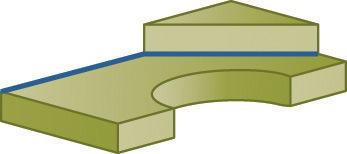
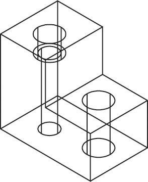
The term apparent intersection refers to lines that appear to intersect in a 2D view or on a computer monitor but actually do not touch, as shown in Figure 4.52. When you look at a wireframe view of a model, the 2D view may show lines crossing each other when, in fact, the lines do not intersect in 3D space. Changing the view of the model can help you determine whether an intersection is actual or apparent.
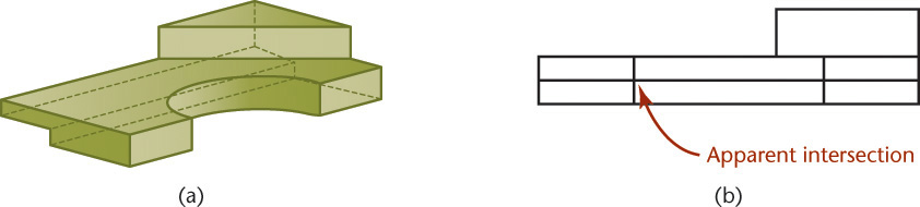
4.52 Apparent Intersection. From the shaded view of this model in (a), it is clear that the back lines do not intersect the half-circular shape. In the wireframe front view in (b), the lines appear to intersect.
Two entities are tangent if they touch each other but do not intersect, even if extended to infinity, as shown in Figure 4.53. A line that is tangent to a circle will have only one point in common with the circle.
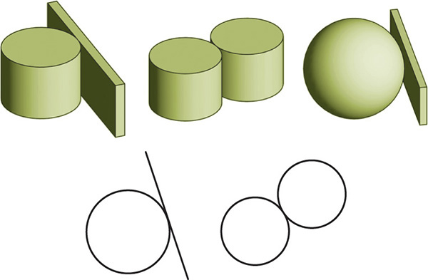
4.53 Tangency. Lines that are tangent to an entity have one point in common but never intersect. 3D objects may be tangent at a single point or along a line.
When a line is tangent to a circle, a radial line from the center of the circle is perpendicular at the point of tangency, as shown in Figure 4.54. Knowing this can be useful in creating sketches and models.
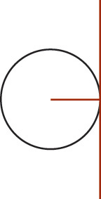
4.54 A radial line from the point where a line is tangent to a circle will always be perpendicular to that line.
The regular geometry of points, lines, circles, arcs, and ellipses is the foundation for many CAD drawings that are created from these types of entities alone. Figure 4.55 shows a 2D CAD drawing that uses only lines, circles, and arcs to create the shapes shown. Figure 4.56 shows a 3D wireframe model that is also made entirely of lines, circles, and arcs. Many complex-looking 2D and 3D images are made solely from combinations of these shapes. Recognizing these shapes and understanding the many ways you can specify them in the CAD environment are key modeling skills.

4.16 Solid Primitives
Many 3D objects can be visualized, sketched, and modeled in a CAD system by combining simple 3D shapes or primitives. They are the building blocks for many solid objects. You should become familiar with these common shapes and their geometry. The same primitives that are useful when sketching objects are also used to create 3D models of those objects.
A common set of primitive solids used to build more complex objects is shown in Figure 4.57. Which of these objects are polyhedra? Which are bounded by single-curved surfaces? Which are bounded by double-curved surfaces? How many vertices do you see on the cone? How many on the wedge? How many edges do you see on the box? Familiarity with the appearance of these primitive shapes when shown in orthographic views can help you in interpreting drawings and in recognizing features that make up objects. Figure 4.58 shows the primitives in two orthographic views. Review the orthographic views and match each to the isometric of the same primitive shown in Figure 4.57.
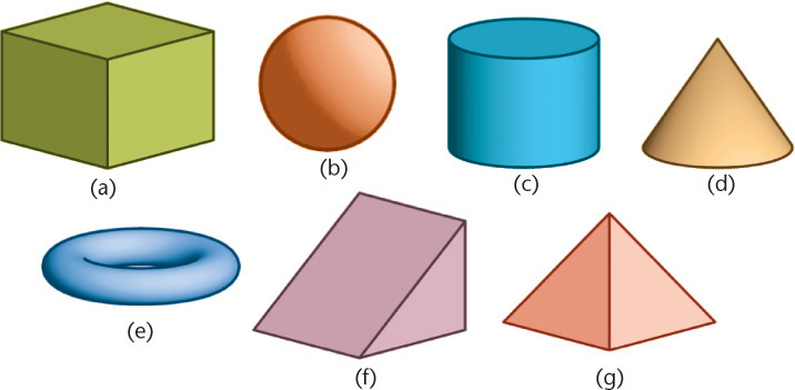
4.57 Solid Primitives. The most common solid primitives are (a) box, (b) sphere, (c) cylinder, (d) cone, (e) torus, (f) wedge, and (g) pyramid.

4.58 Match the top and front views shown here with the primitives shown in Figure 4.57.
Look around and identify some solid primitives that make up the shapes you see. The ability to identify the primitive shapes can help you model features of the objects using a CAD system (see Figure 4.59). Also, knowing how primitive shapes appear in orthographic views can help you sketch these features correctly and read drawings that others have created.

4.59 Complex Shapes. The 3D solid primitives in this illustration show basic shapes that make up a telephone handset. (Photo copyright Everything/Shutterstock.)
Making Complex Shapes with Boolean Operations
Boolean operations, common to most 3D modelers, allow you to join, subtract, and intersect solids. Boolean operations are named for the English mathematician George Boole, who developed them to describe how sets can be combined. Applied to solid modeling, Boolean operations describe how volumes can be combined to create new solids.
The three Boolean operations, defined in Table 4.1, are
• Union (join/add)
• Difference (subtract)
• Intersection
Name |
Definition |
Venn Diagram |
Union (join/add) |
The volume in both sets is combined or added. Overlap is eliminated. Order does not matter: A union B is the same as B union A. |
|
Difference (subtract) |
The volume from one set is subtracted or eliminated from the volume in another set. The eliminated set is completely eliminated—even the portion that does not overlap the other volume. The order of the sets selected when using difference does matter (see Figure 4.60). A subtract B is not the same as B subtract A. |
|
Intersection |
The volume common to both sets is retained. Order does not matter: |
|
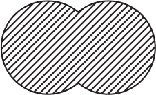
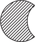

Figure 4.61 illustrates the result of the Boolean operations on three pairs of solid models. Look at some everyday objects around you and make a list of the primitive solid shapes and Boolean operations needed to make them.

4.60 Order Matters in Subtraction. The models here illustrate how A – B differs significantly from B – A.
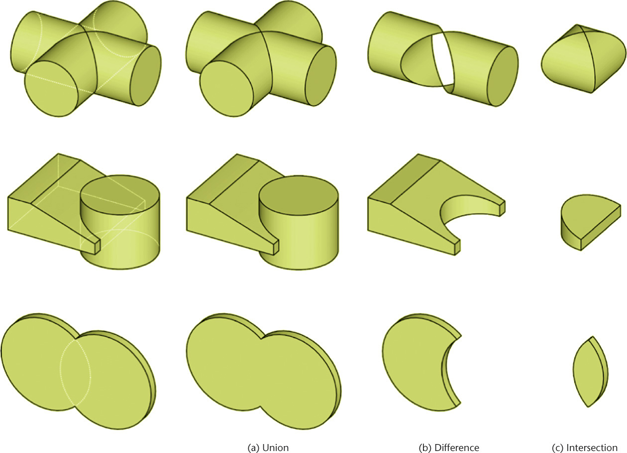
4.61 Boolean Operations. The three sets of models at left produce the results shown at right when the two solids are (a) unioned, (b) subtracted, and (c) intersected.
Figure 4.62 shows a bookend and a list of the primitives available in the CAD system used to create it, along with the Boolean operations used to make the part.
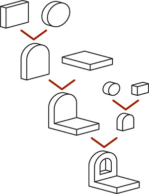
4.62 Shapes in a Bookend. This diagram shows how basic shapes were combined to make a bookend. The box and cylinder at the top were unioned, then the resulting end piece and another box were unioned. To form the cutout in the end piece, another cylinder and box were unioned, then the resulting shape was subtracted from the end piece.
4.17 Recognizing Symmetry
An object is symmetrical when it has the same exact shape on opposite sides of a dividing line (or plane) or about a center or axis. Recognizing the symmetry of objects can help you in your design work and when you are sketching or using CAD to represent an object. Figure 4.63 shows a shape that is symmetrical about several axes of symmetry (of which two are shown) as well as about the center point of the circle.

Mirrored shapes have symmetry where points on opposite sides of the dividing line (or mirror line) are the same distance away from the mirror line. For a 2D mirrored shape, the axis of symmetry is the mirror line. For a 3D mirrored shape, the symmetry is about a plane. Examples of 3D mirrored shapes are shown in Figure 4.64.

4.64 3D Mirrored Shapes. Each of these symmetrical shapes has two mirror lines, indicated by the thin axis lines. To create one of these parts, you could model one quarter of it, mirror it across one of the mirror lines, then mirror the resulting half across the perpendicular mirror line.
To simplify sketching, you need to show only half the object if it is symmetrical (Figure 4.65). A centerline line pattern provides a visual reference for the mirror line on the part.
Most CAD systems have a command available to mirror existing features to create new features. You can save a lot of modeling time by noticing the symmetry of the object and copying or mirroring the existing geometry to create new features.
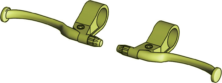
Right- and Left-Hand Parts
Many parts function in pairs for the right and left sides of a device. A brake handle for the left side of a mountain bike is a mirror image of the brake handle for the right side of the bike (Figure 4.66). Using CAD, you can create the part for the left side by mirroring the entire part. On sketches you can indicate a note such as RIGHT-HAND PART IS SHOWN. LEFT-HAND PART IS OPPOSITE. Right-hand and left-hand are often abbreviated as RH and LH in drawing notes.
Tip
Using symmetry when you model can be important when the design requires it. When the design calls for symmetrical features to be the same, mirroring the feature ensures that the two resulting features will be the same.
Parting-Line Symmetry
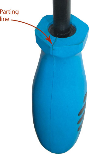
Molded symmetrical parts are often made using a mold with two halves, one on each side of the axis of symmetry. The axis or line where two mold parts join is called a parting line. When items are removed from a mold, sometimes a small ridge of material is left on the object. See if you can notice a parting line on a molded object such as your toothbrush or a screwdriver handle such as the one shown in Figure 4.67. Does the parting line define a plane about which the object is symmetrical? Can you determine why that plane was chosen? Does it make it easier to remove the part from the mold? As you are developing your sketching and modeling skills think about the axis of symmetry for parts and how it could affect their manufacture.

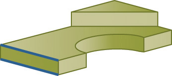
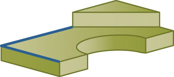
4.18 Extruded Forms
Extrusion is the manufacturing process of forcing material through a shaped opening (Figure 4.69). Extrusion in CAD modeling creates a 3D shape in a way similar to the extrusion manufacturing process. This modeling method is common even when the part will not be manufactured as an extrusion.

4.69 Extruded Shape. Symmetry and several common geometric shapes were used to create this linear guide system. The rail in (a) was created by forcing aluminum through an opening with the shape of its cross section. The extruded length was then cut to the required length. The solid model in (c) was created by defining the 2D cross-sectional shape (b) and specifying a length for the extrusion. (Integrated configuration of Integral V™ linear guides courtesy of PBCLinear.)
To create as shape by extrusion, sketch the 2D outline of the basic shape of the object (usually called a profile), and then specify the length for the extrusion. Most 3D CAD systems provide an Extrude command. Some CAD systems allow a taper (or draft) angle to be specified to narrow the shape over its length (Figure 4.70).
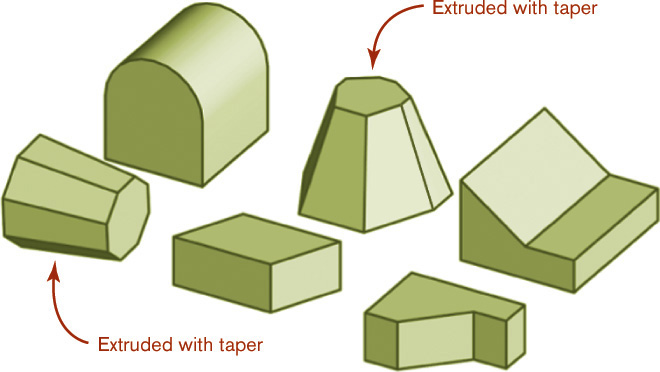
4.70 These CAD models were formed by extruding a 2D outline. Two of the models were extruded with a taper.
Swept Shapes
A swept form is a special case of an extruded form. Sweeping describes extruding a shape along a curved path. To sweep a shape in CAD, create the 2D profile and a 2D or 3D curve to serve as the path. Some swept shapes are shown in Figure 4.71.
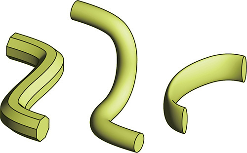
4.71 Swept Shapes. These shapes started as an octagon, a circle, and an ellipse, then were swept along a curved path.
Spotlight: Sketching Extruded Shapes
Shapes that can be created using extrusion are often easily sketched as oblique projections. To sketch extruded shapes, show the shape (or profile) that will be extruded parallel to the front viewing plane in the sketch. Copy this same shape over and up in the sketch based on the angle and distance you want to use to represent the depth. Then, sketch in the lines for the receding edges.

4.19 Revolved Forms
Revolution creates 3D forms from basic shapes by revolving a 2D profile around an axis to create a closed solid object. To create a revolved solid, create the 2D shape to be revolved, specify an axis about which to revolve it, then indicate the number of degrees of revolution. Figure 4.72 shows some shapes created by revolution.

4.72 Revolved Shapes. Each of the solids shown here was created by revolving a 2D shape around an axis.
Often, a 2D sketch is used to create 3D CAD models. Look at the examples shown in Figure 4.73 and match them to the 2D profile used to create the part. For each part, decide whether extrusion, revolution, or sweeping was used to create it.

4.20 Irregular Surfaces
Not every object can be modeled using the basic geometric shapes explored in this chapter. Irregular surfaces are those that cannot be unfolded or unrolled to lie in a flat plane. Solids that have irregular or warped surfaces cannot be created merely by extrusion or revolution. These irregular surfaces are created using surface modeling techniques. Spline curves are frequently the building blocks of the irregular surfaces found on car and snowmobile bodies, molded exterior parts, aircraft, and other (usually exterior) surfaces of common objects, such as an ergonomic mouse. An example of an irregular surface is shown in Figure 4.74. You will learn more about modeling irregular surfaces in Chapter 5.
4.21 User Coordinate Systems
Most CAD systems allow you to create your own coordinate systems to aid in creating drawing geometry. These are often termed user coordinate systems (in AutoCAD, for example) or local coordinate systems, in contrast with the default coordinate system (sometimes called the world coordinate system or absolute coordinate system) that is used to store the model in the drawing database. To use many CAD commands effectively, you must know how to orient a user coordinate system.
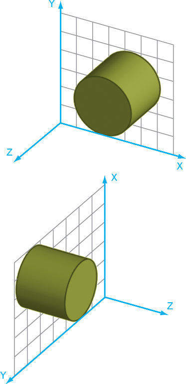
Most CAD systems create primitive shapes the same way each time with respect to the current X-, Y-, and Z-directions. For example the circular shape of the cylinder is always in the current X-Y plane, as shown in Figure 4.75.

4.75 Cylnder Construction. The cylinder is created with the circular base on the X-Y plane and the height in Z.
To create a cylinder oriented differently, create a user coordinate system in the desired orientation (Figure 4.76).
Tip
All CAD systems have a symbol that indicates the location of the coordinate axes—both the global one used to store the model and any user-defined one that is active. Explore your modeler so you are familiar with the way it indicates each.
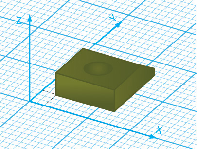
To create the hole perpendicular to the oblique surface shown in Figure 4.77, create a new local coordinate system aligned with the inclined surface. After you have specified the location of the hole using the more convenient local coordinate system, the CAD software translates the location of the hole to the world (default) coordinate system.

4.77 Drawing on an Inclined Plane. A new coordinate system is defined relative to the slanted surface to make it easy to create the hole.
Many CAD systems have a command to define the plane for a user coordinate system by specifying three points. This is often an easy way to orient a new coordinate system—especially when it needs to align with an oblique or inclined surface. Other solid modeling systems allow the user to select an existing part surface on which to draw the new shape. This is analogous to setting the X-Y plane of the user coordinate system to coincide with the selected surface. With constraint-based modelers a “sketch plane” often is selected on which a basic shape is drawn that will be used to form a part feature. This defines a coordinate system for the sketch plane.
A user or local coordinate system is useful for creating geometry in a model. Changing the local coordinate system does not change the default coordinate system where the model data are stored.
4.22 Transformations
A 3D CAD package uses the default Cartesian coordinate system to store information about the model. One way it may be stored is as a matrix (rows and columns of numbers) representing the vertices of the object. Once the object is defined, the software uses mathematical methods to transform the matrix (and the object) in various ways. There are two basic kinds of transformations: those that transform the model itself (called geometric transformations) and those that merely change the view of the model (called viewing transformations).
Geometric Transformations
The model stored in the computer is changed using three basic transformations (or changes): moving (sometimes called translation), rotating, and scaling. When you select a CAD command that uses one of these transformations, the CAD data stored in your model are converted mathematically to produce the result. Commands such as Move (or Translate), Rotate, and Scale transform the object on the coordinate system and change the coordinates stored in the 3D model database.
Figure 4.78 shows a part after translation. The model was moved over 2 units in the X-direction and 3 units in the Y-direction. The corner of the object is no longer located at the origin of the coordinate system.

4.78 Translation. This model has been moved 2 units in the X-direction and 3 units in the Y-direction.
Figure 4.79 illustrates the effect of rotation. The rotated object is situated at a different location in the coordinate system. Figure 4.80 shows the effect of scaling. The scaled object is larger dimensionally than the previous object.

Tip
The following command names are typically used when transforming geometry:
• Move
• Rotate
• Scale
Viewing Transformations
A viewing transformation does not change the coordinate system or the location of the model on the coordinate system; it simply changes your view of the model. The model’s vertices are stored in the computer at the same coordinate locations no matter the direction from which the model is viewed on the monitor (Figure 4.81).

4.81 Changing the View. Note that the location of the model relative to the coordinate axes does not change in any of the different views. Changing the view does not transform the model itself.
Although the model’s coordinates do not change when the view does, the software does mathematically transform the model database to produce the new appearance of the model on the screen. This viewing transformation is stored as a separate part of the model file (or a separate file) and does not affect the coordinates of the stored model. Viewing transformations change the view on the screen but do not change the model relative to the coordinate system.
Common viewing transformations are illustrated in Figure 4.82. Panning moves the location of the view on the screen. If the monitor were a hole through which you were viewing a piece of paper, panning would be analogous to sliding the piece of paper to expose a different portion of it through the hole. Zooming enlarges or reduces the view of the objects and operates similar to a telephoto lens on a camera. A view rotation is actually a change of viewpoint; the object appears to be rotated, but it is your point of view that is changing. The object itself remains in the same location on the coordinate system.

4.82 Common View Transformations. Panning moved the view of the objects in (a) to expose a different portion of the part in (b). In (c), the view is enlarged to show more detail. In (d), the view is rotated to a different line of sight. In each case, the viewing transformation applies to all the objects in the view and does not affect the location of the objects on the coordinate system. (Notice that the position relative to the coordinate system icon does not change.)
Viewing controls transform only the viewing transformation file, changing just your view. Commands to scale the object on the coordinate system transform the object’s coordinates in the database.
Examine the six models and their coordinates in Figure 4.83. Which are views that look different because of changes in viewing controls? Which look different because the objects were rotated, moved, or scaled on the coordinate system?
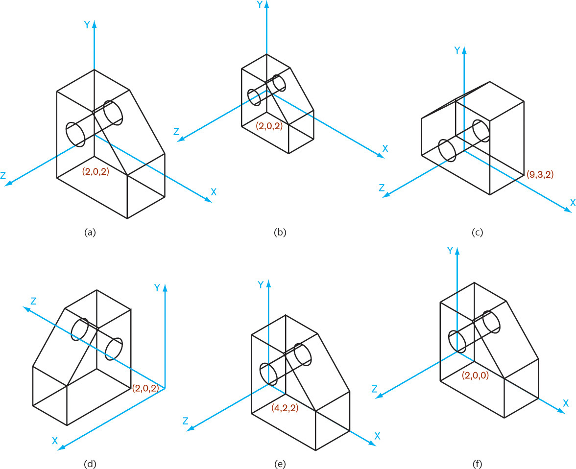
4.83 Geometric or Viewing Transformation? Three of these models are the same, but the viewing location, zoom, or rotation has changed. Three have been transformed to different locations on the coordinate system.
You will use the basic geometric shapes and concepts outlined in this chapter to build CAD models and create accurate freehand sketches. The ability to visualize geometric entities on the Cartesian coordinate system will help you manipulate the coordinate system when modeling in CAD.
Tip
The following are typical command names for view transformations:
• Pan
• Spin (or Rotate View)
• Zoom
Industry Case: The Geometry of 3D Modeling: Use the Symmetry
Strategix ID used magnets to create a clean, quiet, zero maintenance brake for the exercise bike it designed for Park City Entertainment. When copper rings on the bike’s iron flywheel spin past four rare-earth magnets, they create current in circular flow (an eddy current) that sets up a magnetic field.
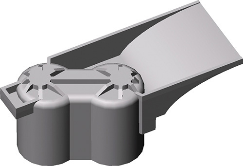
This opposing magnetic field dissipates power and slows the wheel. Moving the magnets onto and off the copper rings varies the amount of resistance delivered. When Marty Albini, Senior Mechanical Engineer, modeled the plastic magnet carrier for the brake, he started with the magnets and their behavior as the carrier moved them onto and off the copper rings (see Figure 4.84). “There is no one way to think about modeling a part,” Albini said. “The key is to design for the use of the part and the process that will be used to manufacture it.” To make the magnet carrier symmetrical, Albini started by modeling half of it.
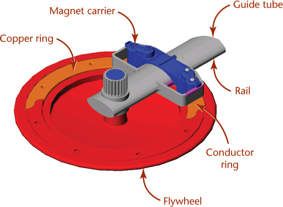
4.84 Flywheel Assembly. The magnet carrier for the brake was designed to move onto and off the conductor ring by sliding along an elliptical guide tube, pulled by a cable attached to the small tab in the middle of the carrier.
The magnet carrier was designed as a part in the larger flywheel assembly, parts of which were already completed.
Each pair of magnets was attached to a backing bar that kept them a fixed distance apart. To begin, Albini started with the geometry he was sure of: the diameter of the magnets, the space between them, and the geometry of the conductor ring. He sketched an arc sized to form a pocket around one of the magnets so that its center point would be located on the centerline of the conductor ring (see Figure 4.85). He then sketched another similar arc but with its center point positioned to match the distance between the centers of the two magnets. He connected the two arcs with parallel lines to complete the sketch of the inside of the carrier. This outline was offset to the outside by the thickness of the wall of the holder. (Because this is an injection-molded plastic part, a uniform wall thickness was used throughout.) One final constraint was added to position the carrier against the rail on the elliptical tube along which it would slide: the outside of the inner arc is tangent to this rail. With the sketch geometry fully defined, Albini extruded the sketch up to the top of the guide tube and down to the running clearance from the copper ring.

4.85 Extruding the Carrier. The magnet carrier was extruded up and down from the sketch, shown here as an outline in the middle of the extruded part. Notice that the sketch is tangent to the guide tube rail, and the centers of the arcs in the sketch are located on the centerline of the conductor ring.
To add a lid to the holder, Albini used the SolidWorks Offset command to trace the outline of the holder. First, he clicked on the top of the holder to make its surface the active sketch plane. This is equivalent to changing the user coordinate system in other packages: it signals to SolidWorks that points picked from the screen lie on this plane. He then selected the top edges of the holder and used the Offset command with a 0 offset to “trace” the outline as a new sketch. To form the lid, he extruded the sketch up (in the positive Z-direction) the distance of the uniform wall thickness.
SolidWorks joined this lid to the magnet holder automatically because both features are in the same part and have surfaces that are coincident. This built-in operation is similar to a Boolean join in that the two shapes are combined to be one.
For the next feature, Albini created a “shelf” at the height of the rail on which the holder will slide. Using Offset again, he traced the outline of the holder on the sketch plane, then added parallel and perpendicular lines to sketch the outline of the bottom of the shelf. The outline was then extruded up by the wall thickness. The distance from the outside of the magnet holder to the edge of the shelf created a surface that would sit on the rail (see Figure 4.86).

4.86 Changing the Sketch Plane. The surface of the rail was used as the sketch plane for the “shelf” on which the magnet carrier will slide.
Two walls were added by offsetting the edge of the shelf toward the magnet holder by the wall thickness, then offsetting the edge again by 0. Lines were added to connect the endpoints into an enclosed shape to be extruded. (In Solid-Works, an extrusion can be specified to extend in one or both directions, and to extend to a vertex, a known distance, the next surface, or the last surface encountered.) For the walls, Albini extruded them to the top surface of the magnet holder “lid.”
The connecting web between the magnet holders needed to match the shape of the elliptical tube in the flywheel assembly (see Figure 4.87). To make it, Albini sketched an ellipse on the newly created wall. An ellipse is a sketching primitive that can be specified by entering the length of the major and minor axes. Albini used the dimensions from the tube for the first ellipse sketch, then drew a second one with the same center point but with longer axes so that a gap equal to the wall thickness between them would be formed. The two ellipses were trimmed off at the bottom surface of the shelf and at the midpoint, and lines were drawn to make a closed outline. The finished sketch was extruded to the outside surface of the opposite wall.

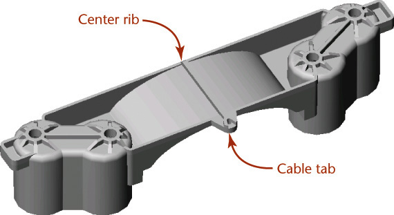
4.87 This view of the magnet carrier shows the elliptical shape of the connecting web and the rectangular shape of the tab. The parting line for the part, shown here as a dotted white line, is located at the edge of the fillet on the top of the magnet chambers.
More walls were sketched and extruded from the bottom surface of the shelf. Then, the wall over the connecting web was sketched and extruded down to the web.
The next step was to add the rounded edges for the top of the magnet holder. Albini invoked the Fillet command and selected to round all the edges of the top surface at once. As it created the fillet, SolidWorks maintained the relationship between the wall surfaces that intersected the top edge of the holder and extended them to the new location of the edge.
Next, Albini created a tab at the end of the part that would rest on the plastic collar in the assembly that went all the way around the magnet carrier. He first extruded a rectangular shape up from the top of the collar to form the “floor” of the tab. The walls of the tab required two additional extrusions.
The fillet at the top of the magnet holder provided the location for the parting line—the line where the two halves of the mold would come apart and release the part. Albini added a parting plane and used the built-in Draft option to add taper to the part so it would come out of the mold. After selecting all the surfaces below the parting plane, he specified a draft angle, and SolidWorks adjusted all the surfaces. This feature of SolidWorks makes it easy to add the draft angle after a part is finished. When draft is added, the geometry of the part becomes more complex and harder to work with. A cylinder with draft added becomes a truncated cone, for example, and the angles at which its edges intersect other edges vary along its length.
The next step was to add the bosses at the top of the magnet chambers that would support the bolts controlling the depth of the magnets. As it was a design goal to make the top of the chamber as stiff as possible to limit flex caused by the attraction of the magnets to the flywheel, the bosses were placed as far apart as possible, and ribs were added for rigidity. The bosses were sketched as circles on the top surface of the magnet holder with their centers concentric with the holes in the bar connecting the magnets below. Both bosses were extruded up in the same operation.

4.88 Bosses and Ribs. Sketched circles were extruded to form the bosses on the top of the magnet chamber. The dotted lines shown here on the top of the chamber pass through the center point of the bosses and were used to locate the center rib and radial ribs.
Ribs in SolidWorks are built-in features. To create a rib, you simply draw a line and specify a width, and SolidWorks creates the rib and ends it at the first surface it encounters. To create the center rib, Albini sketched a line on the plane at the top of the bosses and specified a width (ribs on a plastic part are usually two thirds of the thickness of the walls). The rib was formed down to the top surface of the holder lid. For the ribs around the bosses, Albini did as Obi Wan Kenobi might have advised: “Use the symmetry, Luke.” He sketched the lines for ribs radially from the center points of the bosses (see Figure 4.88). To create the ribs, Albini created four of them on one boss, then mirrored them once to complete the set for one boss, then mirrored all the ribs from one boss to the other boss. Once all the ribs were formed, he cut the tops off the ribs and bosses to achieve the shape shown in Figure 4.89.
4.89 This view of the magnet carrier shows the symmetry of the ribs and the shape that resulted from “slicing off” the top of the bosses after the ribs were formed.
The result was a stiffer rib and a shape that could not be achieved with a single rib operation. To complete the part, circles were drawn concentric to the bosses and extruded to form holes that go through the part (see Figure 4.90). Draft was added to the ribs and walls to make the part release from the mold easily. Fillets were added to round all the edges, reducing stresses and eliminating hot spots in the mold. Then, the part was mirrored to create the other half. The center rib and tab for attaching the cable were added and more edges filleted. Draft was added to the inside of the holder, and the part was complete.
4.90 Circles concentric with the bosses were extruded to form the holes before the part was mirrored and remaining features added to finish the magnet carrier.
(Images courtesy of Marty Albini. This case study is provided as a courtesy by the owner of the intellectual property rights, Park City Entertainment. All rights reserved.)
CAD at Work: Defining Drawing Geometry
2D CAD programs may allow drawing geometry to be controlled through constraints or parametric definitions. AutoCAD is one software platform that now provides this tool. In AutoCAD, constraints are associations that can be applied to 2D geometry to restrict how the drawing behaves when a change is made.
Constraints are of two types:
• Geometric constraints create geometric relationships between drawing objects, such as requiring that a circle remain tangent to a line, even when its radius is updated.
• Dimensional constraints define distances, angles, and radii for drawing objects. These dimensional constraints typically can also be defined by equations, making them a powerful tool.
Usually, it is best to define the geometric constraints first and then apply dimensional constraints. This way the essential geometry of the shape is defined, and the dimensions can be changed as the size requirements vary.
Figure A shows an AutoCAD drawing that uses fixed and tangent constraints. The fixed constraint allows you to force a drawing object to stay in a permanent location on the coordinate system. The tangent constraint defines a relationship between two drawing objects, such as circles, arcs, and lines.

(A) AutoCAD provides tools for defining geometric and dimensional constraints to control drawing geometry. (Autodesk screen shots reprinted courtesy of Autodesk, Inc.)
Understanding geometric relationships is a key skill for creating drawings that use parametric constraints. When geometric constraints are applied awkwardly or when the software does not provide a robust tool for constraining the shape, it can be difficult to get good results when updating drawings.
Chapter Summary
• Understanding how to produce accurate geometry is required for technical drawings whether constructed by hand or using a CAD system.
• All drawings are made up of points, lines, arcs, circles, and other basic elements in relation to each other. Whether you are drawing manually or using CAD, the techniques are based on the relationships between basic geometric elements.
• CAD systems often produce the same result as a complicated hand construction technique in a single step. A good understanding of drawing geometry helps you produce quick and accurate CAD drawings as well as manual drawings.
Skills Summary
You should be able to convert and interpret different coordinate formats used to describe point locations and be familiar with some of the basic geometry useful in creating CAD drawings. You should also be able to identify and sketch primitive shapes joined by Boolean operations. In addition, you should be able to visualize and sketch revolved and extruded shapes. The following exercises will give you practice using all these skills.
Review Questions
1. What tools are useful for drawing straight lines?
2. What tools are used for drawing arcs and circles?
3. How many ways can an arc be tangent to one line? To two lines? To a line and an arc? To two arcs? Draw examples of each.
4. Draw an approximate ellipse with a major diameter of 6″ and a minor diameter of 3″ . Draw a second approximate ellipse with a major diameter of 200 mm and a minor diameter of 100 mm.
5. Give one example of a construction technique for CAD that requires a good understanding of drawing geometry.
6. What is typical accuracy for manually created drawings?
7. What accuracies may be possible using a CAD system?
8. Sketch some objects that you use or would design that have right-hand and left-hand parts, such as a pair of in-line skates or side-mounted stereo computer speakers.
9. In solid modeling, simple 3D shapes are often used to create more complex objects. These are called primitives. Using an isometric grid, draw seven primitives.
10. What is a Boolean operation? Define two Boolean operations by sketching an example of each in isometric view.
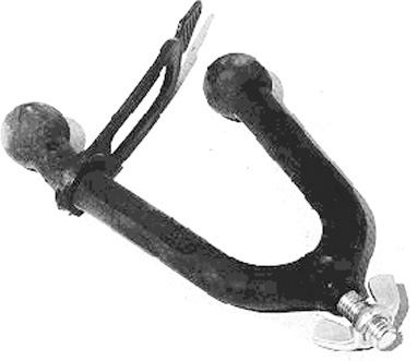
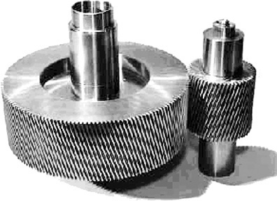
11. Consider primitives and Boolean operations that could be used to create a “rough” model of each of the items shown below. Using the photos as underlays, sketch primitives that could be used to create items a–d.
a. Handlebar-mount gun rack
b. ACME Corporation reduction gear
c. Ashcroft Model 1305D deadweight pressure tester

d. Davis Instruments solar-powered digital thermometer

12. Use nothing but solid primitives to create a model of a steam locomotive. Sketch the shapes and note the Boolean operations that would be used to union, difference, or intersect them, or create the model using Boolean operations with your modeling software. Use at least one box, sphere, cylinder, cone, torus, wedge, and pyramid in your design.
Exercise 4.2 Draw any angle. Label its vertex C. Bisect the angle and transfer half the angle to place its vertex at arbitrary point D.
Exercise 4.3 Draw an inclined line EF. Use distance GH equal to 42 mm. Draw a new line parallel to EF and distance GH away.
Exercise 4.4 Draw line JK 95 mm long. Draw a second line LM 58 mm long. Divide JK into five equal parts. Use a different method than you selected to divide line JK to divide line LM into three equal parts.
Exercise 4.5 Draw line OP 92 mm long. Divide it into three proportional parts with the ratio 3:5:9.
Exercise 4.6 Draw a line 87 mm long. Divide it into parts proportional to the square of x, where x = 1, 2, 3, and 4.
Exercise 4.7 Draw a triangle with the sides 76 mm, 85 mm, and 65 mm. Bisect the three interior angles. The bisectors should meet at a point. Draw a circle inscribed in the triangle, with the point where the bisectors meet as its center.
Exercise 4.8 Draw a right triangle that has a hypotenuse of 65 mm and one leg 40 mm. Draw a circle through the three vertices.
Exercise 4.9 Draw inclined line QR 84 mm long. Mark point P on the line 32 mm from Q. Draw a line perpendicular to QR at point P. Select any point S 45.5 mm from line QR. Draw a line perpendicular from S to line QR.
Exercise 4.10 Draw two lines forming an angle of 35.5°.
Exercise 4.11 Draw two lines forming an angle of 33.16°.
Exercise 4.12 Draw an equilateral triangle with sides of 63.5 mm. Bisect the interior angles. Draw a circle inscribed in the triangle.
Exercise 4.13 Draw an inclined line TJ 55 mm long. Using line TJ as one of the sides, construct a square.
Exercise 4.14 Create a 54-mm-diameter circle. Inscribe a square in the circle, and circumscribe a square around the circle.
Exercise 4.15 Create a 65-mm-diameter circle. Find the vertices of an inscribed regular pentagon. Join these vertices to form a five-pointed star.
Exercise 4.16 Create a 65-mm-diameter circle. Inscribe a hexagon, and circumscribe a hexagon.
Exercise 4.17 Create a square with 63.5 mm sides. Inscribe an octagon.
Exercise 4.18 Draw a triangle with sides 50 mm, 38 mm, and 73 mm. Copy the triangle to a new location and rotate it 180°.
Exercise 4.19 Make a rectangle 88 mm wide and 61 mm high. Scale copies of this rectangle, first to 70 mm wide and then to 58 mm wide.
Exercise 4.20 Draw three points spaced apart randomly. Create a circle through the three points.
Exercise 4.21 Draw a 58-mm-diameter circle. From any point S on the left side of the circle, draw a line tangent to the circle at point S. Create a point T, to the right of the circle and 50 mm from its center. Draw two tangents to the circle from point T.

Exercise 4.22 Open-Belt Tangents. Draw a horizontal centerline near the center of the drawing area. On this centerline, draw two circles spaced 54 mm apart, one with a diameter of 50 mm, the other with a diameter of 38 mm. Draw “open-belt”-style tangents to the circles.

Exercise 4.23 Crossed-Belt Tangents. Use the same instructions as Exercise 4.22, but for “crossed-belt”-style tangents.
Exercise 4.24 Draw a vertical line VW. Mark point P 44 mm to the right of line VW. Draw a 56-mm-diameter circle through point P and tangent to line VW.
Exercise 4.25 Draw a vertical line XY. Mark point P 44 mm to the right of line XY. Mark point Q on line XY and 50 mm from P. Draw a circle through P and tangent to XY at point Q.
Exercise 4.26 Draw a 64-mm-diameter circle with center C. Create point P to the lower right and 60 mm from C. Draw a 25-mm-radius arc through P and tangent to the circle.
Exercise 4.27 Draw intersecting vertical and horizontal lines, each 65 mm long. Draw a 38-mm-radius arc tangent to the two lines.
Exercise 4.28 Draw a horizontal line. Create a point on the line. Through this point, draw a line upward to the right at 60° from horizontal. Draw 35-mm-radius arcs in an obtuse and an acute angle tangent to the two lines.
Exercise 4.29 Draw two intersecting lines to form a 60° angle. Create point P on one line a distance of 45 mm from the intersection. Draw an arc tangent to both lines with one point of tangency at P.
Exercise 4.30 Draw a vertical line AB. In the lower right of the drawing, create a 42-mm-radius arc with its center 75 mm to the right of the line. Draw a 25-mm-radius arc tangent to the first arc and to line AB.
Exercise 4.31 With centers 86 mm apart, draw arcs of radii 44 mm and 24 mm. Draw a 32-mm-radius arc tangent to the two arcs.
Exercise 4.32 Draw a horizontal centerline near the center of the drawing area. On this centerline, draw two circles spaced 54 mm apart, one with a diameter of 50 mm, the other with a diameter of 38 mm. Draw a 50-mm-radius arc tangent to the circles and enclosing only the smaller one.
Exercise 4.33 Draw two parallel inclined lines 45 mm apart. Mark a point on each line. Connect the two points with an ogee curve tangent to the two parallel lines. (An ogee curve is a curve tangent to both lines.)
Exercise 4.34 Draw a 54-mm-radius arc that subtends an angle of 90°. Find the length of the arc.
Exercise 4.35 Draw a horizontal major axis 10 mm long and a minor axis 64 mm long to intersect near the center of the drawing space. Draw an ellipse using these axes.
Exercise 4.36 Create six equal rectangles and draw visible lines, as shown. Omit dimensions and instructional notes.
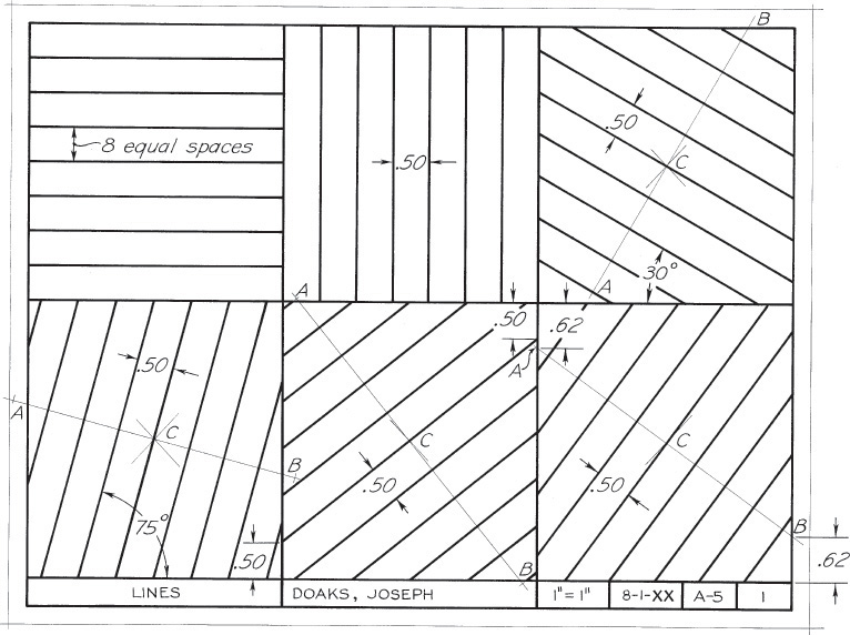
Exercise 4.37 Create six equal rectangles and draw lines as shown. In the first two spaces, draw examples of the standard line patterns used in technical drawings: visible, hidden, construction, centerlines, cutting-plane lines, and phantom. In the remaining spaces, locate centers C by diagonals, and then work constructions out from them. Omit the metric dimensions and instructional notes.

Exercise 4.38 Draw the figures as shown. Omit all dimensions.

Exercise 4.39 Draw the friction plate. Omit dimensions and notes.

Exercise 4.40 Draw the Geneva cam. Omit dimensions and notes.
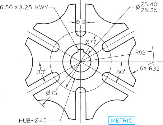
Exercise 4.41 Draw accurately in pencil the shear plate. Give the length of KA. Omit the other dimensions and notes.
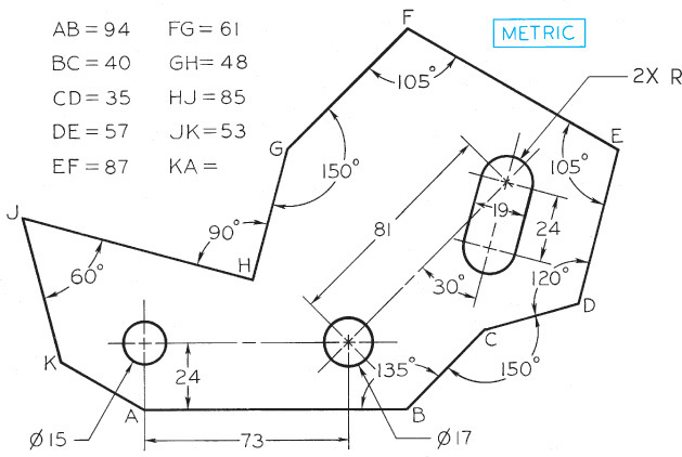
Exercise 4.42 Draw the ratchet wheel using pencil. Omit the dimensions and notes.

Exercise 4.43 Draw the latch plate using pencil. Omit the dimensions and notes.
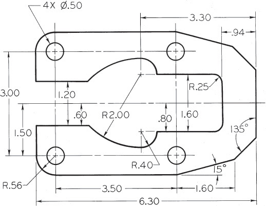
Exercise 4.44 Draw the parabolic floodlight reflector shown.
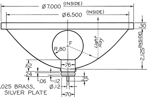
Exercise 4.45 Identify the solid primitives and Boolean operations you could use to create the following objects.
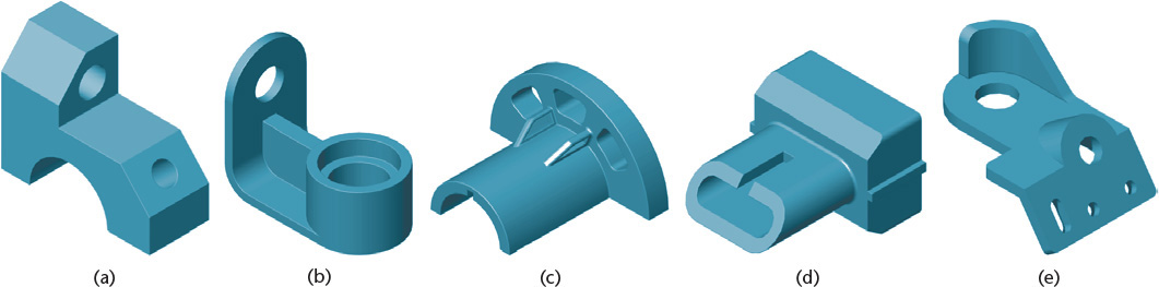
Exercise 4.46 Use an isometric grid to help sketch the solids formed by revolving the following shapes about the axis shown. Coordinates are defined by the X-Y-Z icon, with positive X to the right, positive Y up, and positive Z out of the page.
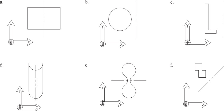
Exercise 4.47 Use an isometric grid to help sketch the solids formed by extruding the following shapes along the axis specified. Coordinates are defined by the X-Y-Z icon, with positive X to the right, positive Y up, and positive Z out of the page.

Exercise 4.48 Starting at point A in each of the figures, list the coordinates for each point in order as relative coordinates from the previous point.
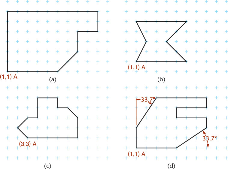
Exercise 4.49 Plot the coordinates in each of the lists on grid paper. Each point represents the endpoint of a line from the previous point, unless otherwise indicated. Relative coordinates are preceded by @.
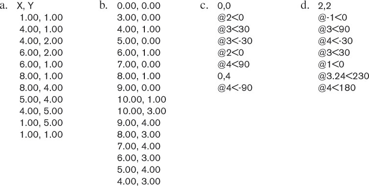
Exercise 4.50 Using the information provided on the drawing, determine the coordinates you would use (absolute, relative, or polar) and the order in which you would enter them to create the figure.

Exercise 4.51 Using the information provided on the drawing, determine the coordinates you would use (absolute, relative, or polar) and the order in which you would enter them to create the figure.
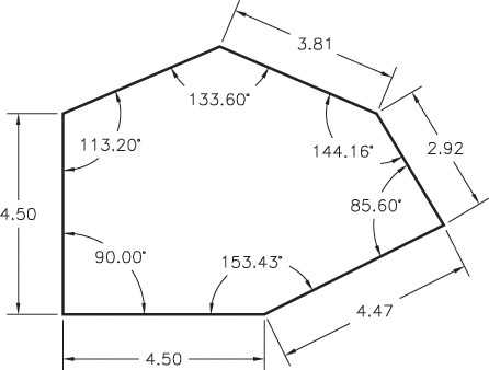
Exercise 4.52 Using the information provided on the drawing, determine the coordinates you would use (absolute, relative, or polar) and the order in which you would enter them to create the figure.