
5 State-of-the-art in deep learning: Transformers
- Representing text in numerical format for machine learning models
- Building a Transformer model using the Keras sub-classing API
We have seen many different deep learning models so far, namely fully connected networks, convolutional neural networks, and recurrent neural networks. We used a fully connected network to reconstruct corrupted images, a convolutional neural network to classify vehicles from other images, and finally an RNN to predict future CO2 concentration values. In this chapter we are going to talk about a new type of model known as the Transformer.
Transformers are the latest generation of deep networks to emerge. Vaswani et al., in their paper “Attention Is All You Need” (https://arxiv.org/pdf/1706.03762.pdf), popularized the idea. They coined the term Transformer and explained how it shows great promise for the future. In the years following, leading tech companies like Google, OpenAI, and Facebook implemented bigger and better Transformer models that have significantly outperformed other models in the NLP domain. Here, we will refer to the model introduced in their paper by Vaswani et al. to learn about it. Although Transformers do exist for other domains (e.g., computer vision), we will focus on how the Transformer is used in the NLP domain, particularly on a machine translation task (i.e., language translation using machine learning models). This discussion will leave out some of the details from the original Transformer paper to improve clarity, but these details will be covered in a later chapter.
Knowing the inner workings of the Transformer model is a must for anyone who wants to excel at using deep learning models to solve real-world problems. As explained, the Transformer model has proliferated the machine learning field quite rapidly. This is mainly because of the performance it has demonstrated in solving complex machine learning problems.
5.1 Representing text as numbers
Say you are taking part in a game show. One challenge in the game is called Word Boxes. There is a matrix of transparent boxes (3 rows, 5 columns, 10 depths). You also have balls with 0 or 1 painted on them. You are given three sentences, and your task is to fill all the boxes with 1s and 0s to represent those sentences. Additionally, you can write a short message (within a minute) that helps someone decipher this later. Later, another team member looks at the boxes and writes down as many words in the original sentences you were initially given.
The challenge is essentially how you can transform text to numbers for machine translation models. This is also an important problem you work on before learning about any NLP model. The data we have seen so far has been numerical data structures. For example, an image can be represented as a 3D array (height, width, and channel dimensions), where each value represents a pixel intensity (i.e., a value between 0 and 255). But what about text? How can we make a computer understand characters, words, or sentences? We will learn how to do this with Transformers in the context of natural language processing (NLP).
You have the following set of sentences:
The first thing you do is assign each word in your vocabulary an ID starting from 1. We will reserve the number 0 for a special token we will see later. Say you assign the following IDs:
After mapping the words to the corresponding IDs, our sentences become the following:
Remember, you need to fill in all the boxes and have a maximum length of 5. Note that our last sentence has six words. This means all the sentences need to be represented by a fixed length. Deep learning models face a similar problem. They process data in batches, and to process it efficiently, the sequence length needs to be fixed for that batch. Real-world sentences can vary significantly in terms of their length. Therefore, we need to
to make them the same length. If we pad the short sentences and truncate long sentences so that the length is 5, we get the following:
Here, we have a 2D matrix of size 3 × 5, which represents our batch of sentences. The final thing to do is represent each of these IDs as vectors. Because our balls have 1s and 0s, you can represent each word with 11 balls (we have 10 different words and the special token <PAD>), where the ball at the position indicated by the word ID is 1 and the rest are 0s. This method is known as one-hot encoding. For example,
0 → [1, 0, 0, 0, 0, 0, 0, 0, 0, 0, 0]
1 → [0, 1, 0, 0, 0, 0, 0, 0, 0, 0, 0]
10 → [0, 0, 0, 0, 0, 0, 0, 0, 0, 1, 0]
11→ [0, 0, 0, 0, 0, 0, 0, 0, 0, 0, 1]
Now you can fill the boxes with 1s and 0s such that you get something like figure 5.1. This way, anyone who has the word for ID mapping (provided in a sheet of paper) can decipher most of the words (except for those truncated) that were initially provided.

Figure 5.1 The boxes in the Word Boxes game. The shaded boxes represent a single word (i.e., the first word in the first sentence, “I,” which has an ID of 1). You can see it’s represented by a single ball of 1 and nine balls of 0.
Again, this is a transformation done to words in NLP problems. You might ask, “Why not feed the word IDs directly?” There are two problems:
-
The value ranges the neural network sees are very large (0-100,000+) for a real-world problem. This will cause instabilities and make the training difficult.
-
Feeding in IDs would falsely indicate that words with similar IDs should be alike (e.g., word ID 4 and 5). This is never the case and would confuse the model and lead to poor performance.
Therefore, it is important to bring words to some vector representation. There are many ways to turn words into vectors, such as one-hot encoding and word embeddings. You have already seen how one-hot encoding works, and we will discuss word embeddings in detail later. When we represent words as vectors, our 2D matrix becomes a 3D matrix. For example, if we set the vector length to 4, you will have a 3 × 6 × 4 3D tensor. Figure 5.2 depicts what the final matrix looks like.
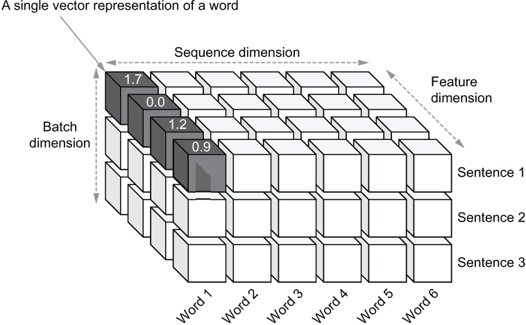
Figure 5.2 3D matrix representing a batch of a sequence of words, where each word is represented by a vector (i.e., the shaded block in the matrix). There are three dimensions: batch, sequence (time), and feature.
Next we will discuss the various components of the popular Transformer model, which will give us a solid grounding in how these models perform internally.
5.2 Understanding the Transformer model
You are currently working as a deep learning research scientist and were recently invited to conduct a workshop on Transformers at a local TensorFlow conference. Transformers are a new family of deep learning models that have surpassed their older counterparts in a plethora of tasks. You are planning to first explain the architecture of the Transformer network and then walk the participants through several exercises, where they will implement the basic computations found in Transformers as sub-classed Keras layers and finally use these to implement a basic small-scale Transformer using Keras.
5.2.1 The encoder-decoder view of the Transformer
The Transformer network is based on an encoder-decoder architecture. The encoder-decoder pattern is common in deep learning for certain types of tasks (e.g., machine translation, question answering, unsupervised image reconstruction). The idea is that the encoder takes an input and maps it to some latent (or hidden) representation (typically smaller), and the decoder constructs a meaningful output using latent representation. For example, in machine translation, a sentence from language A is mapped to a latent vector, from which the decoder constructs the translation of that sentence in language B. You can think of the encoder and decoder as two separate machine learning models, where the decoder depends on the output of the encoder. This process is depicted in figure 5.3. At a given time, both the encoder and the decoder consume a batch of a sequence of words (e.g., a batch of sentences). As machine learning models don’t understand text, every word in this batch is represented by a numerical vector. This is done by following a process such as one-hot encoding, similar to what we discussed in section 5.1.
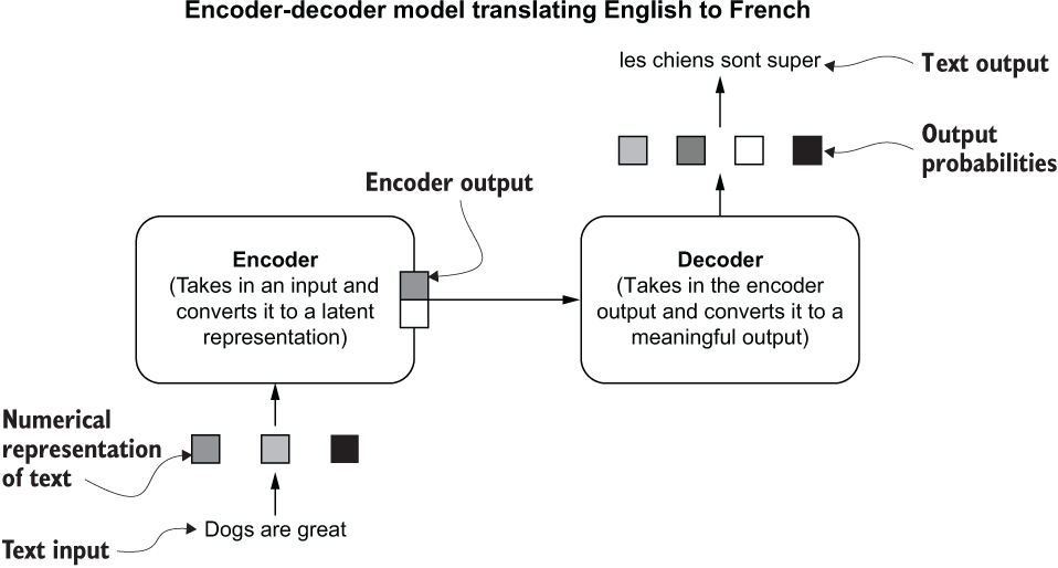
Figure 5.3 The encoder-decoder architecture for a machine translation task
The encoder-decoder pattern is common in real life as well. Say you are a tour guide in France and take a group of tourists to a restaurant. The waiter is explaining the menu in French, and you need to translate this to English for the group. Imagine how you would do that. When the waiter explains the dish in French, you process those words and create a mental image of what the dish is, and then you translate that mental image into a sequence of English words.
Now let’s dive more into the individual components and what they are made of.
5.2.2 Diving deeper
Naturally, you might be asking yourself, “What do the encoder and the decoder consist of?” This is the topic of this section. Note that the encoder and decoder discussed here are quite different from the autoencoder model you saw in chapter 3. As said previously, the encoder and the decoder individually act like multilayered deep neural networks. They consist of several layers, where each layer comprises sublayers that encapsulate certain computations done on inputs to produce outputs. The output of the previous layer feeds as the input to the next layer. It is also important to note that inputs and outputs of the encoder and the decoder are sequences, such as sentences. Each layer within these models takes in a sequence of elements and outputs another sequence of elements. So, what constitutes a single layer in the encoder and the decoder?
Each encoder layer comprises two sublayers:
The self-attention layer produces its final output similarly to a fully connected layer (i.e., using matrix multiplications and activation functions). A typical fully connected layer will take all elements in the input sequence, process them separately, and output an element in place of each input element. But the self-attention layer can select and combine different elements in the input sequence to output a given element. This makes the self-attention layer much more powerful than a typical fully connected layer (figure 5.4).

Figure 5.4 The difference between the self-attention sublayer and the fully connected sublayer. The self-attention sublayer looks at all the inputs in the sequence, whereas the fully connected sublayer only looks at the input that is processed.
Why does it pay to select and combine different input elements this way? In an NLP context, the self-attention layer enables the model to look at other words while it processes a certain word. But what does that mean for the model? This means that while the encoder is processing the word “it” in the sentence “I kicked the ball and it disappeared,” the model can attend to the word “ball.” By seeing both words “ball” and “it” at the same time (learning dependencies), disambiguating words is easier. Such capabilities are of paramount importance for language understanding.
We can understand how self-attention helps us solve a task conveniently through a real-world example. Assume you are playing a game with two people: person A and person B. Person A holds a question written on a board, and you need to speak the answer. Say person A reveals just one word at a time, and after the last word of the question, it is revealed that you are answering the question. For long and complex questions, this is challenging, as you cannot physically see the complete question and have to heavily rely on memory when answering the question. This is what it feels like without self-attention. On the other hand, say person B reveals the full question on the board instead of word by word. Now it is much easier to answer the question, as you can see the whole question at once. If the question is complex and requires a complex answer, you can look at different parts of the question as you provide various sections of the full answer. This is what the self-attention layer enables.
Next, the fully connected layer takes the output elements produced by the self-attention sublayer and produces a hidden representation for each output element in an element-wise fashion. This make the model deeper, allowing it to perform better.
Let’s look in more detail at how data flows through the model in order to better understand the organization of layers and sublayers. Assume the task of translating the sentence “Dogs are great” (English) to “Les chiens sont super” (French). First, the encoder takes in the full sentence “Dogs are great” and produces an output for each word in the sentence. The self-attention layer selects the most important words for each position, computes an output, and sends that information to the fully connected layer to produce a deeper representation. The decoder produces output words iteratively, one after the other. To do that, the decoder looks at the final output sequence of the encoder and all the previous words predicted by the decoder. Assume the final prediction is <SOS> les chiens sont super <EOS>. Here, <SOS> marks the start of the sentence and <EOS> the end of the sentence. The first input it takes is a special tag that indicates the start of a sentence (<SOS>), along with the encoder outputs, and it produces the next word in the translation: “les.” The decoder then consumes <SOS> and “les” as inputs, produces the word “chiens,” and continues until the model reaches the end of the translation (marked by <EOS>). Figure 5.5 depicts this process.
In the original Transformer paper, the encoder has six layers, and a single layer has a self-attention sublayer and a fully connected sublayer, in that order. First, the self-attention layer takes the English words as a time-series input. However, before feeding these words to the encoder, you need to create a numerical representation of each word, as discussed earlier. In the paper, word embeddings (with some additional encoding) are used to represent the words. Each of these embeddings is a 512-long vector. Then the self-attention layer computes a hidden representation for each word of the input sentence. If we ignore some of the implementation details, this hidden representation at time step t can be thought as a weighted sum of all the inputs (in a single sequence), where the weight for position i of the input is determined by how important it is to select (or attend to) the encoder word ewi in the input sequence while processing the word ewt in the encoder input. The encoder makes this decision for every position t in the input sequence. For example, while processing the word “it” in the sentence “I kicked the ball and it disappeared,” the encoder needs to pay more attention to the word “ball” than to the word “the.” The weights in the self-attention sublayer are trained to demonstrate such properties. This way, the self-attention layer produces a hidden representation for each encoder input. We call this the attended representation/output.
The fully connected sublayer then takes over and is quite straightforward. It has two linear layers and a ReLU activation in between the layers. It takes the outputs of the self-attention layer and transforms to a hidden output using
Note that the second layer does not have a nonlinear activation. Next, the decoder has six layers as well, where each layer has three sublayers:
The masked self-attention layer operates similarly to the self-attention layer. However, while processing the sth word (i.e., dws), it masks the words ahead of dws. For example, while processing the word “chiens,” it can only attend to the words “<sos>” and “les.” This is important because the decoder must be able to predict the correct word, given only the previous words it predicted, so it makes sense to force the decoder to attend only to the words it has already seen.
Next, the encoder-decoder attention layer takes the encoder output and the outputs produced by the masked self-attention layer and produce a series of outputs. The purpose of this layer is to compute a hidden representation (i.e., an attended representation) at time s as a weighted sum of encoder inputs, where the weight for position j is determined by how important it is to attend to encoder input e wj, while processing the decoder word dws.
Finally, a fully connected layer identical to the fully connected layer from the encoder layer takes the output of the self-attention layer to produce the final output of the layer. Figure 5.5 depicts the layers and operations discussed in this section at a high level.
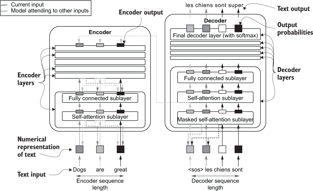
Figure 5.5 Various layers in the encoder and the decoder and various connections formed within the encoder, within the decoder, and between the encoder and the decoder. The squares represent inputs and outputs of the models. The rectangular shaded boxes represent interim outputs of the sublayers.
In the next section, we will discuss what the self-attention layer looks like.
5.2.3 Self-attention layer
We have covered the purpose of the self-attention layer at an abstract level of understanding. It is to, while processing the word wt at time step t, determine how important it is to attend to the ith word (i.e., wi) in the input sequence. In other words, the layer needs to determine the importance of all the other words (indexed by i) for every word (indexed by t). Let’s now understand the computations involved in this process at a more granular level.
First, there are three different entities involved in the computation:
-
A query—The query’s purpose is to represent the word currently being processed.
-
A key—The key’s purpose is to represent the candidate words to be attended to while processing the current word.
-
A value—The value’s purpose is to compute a weighted sum of all words in the sequence, where the weight for each word is based on how important it is for understanding the current word
For a given input sequence, query, key, and value need to be calculated for every position of the input. These are calculated by an associated weight matrix with each entity.
Note that this is an oversimplification of their relationship, and the actual relationship is somewhat complex and convoluted. But this understanding provides the motivation for why we need three different entities to compute self-attention outputs.
Next, we will understand how exactly a self-attention layer goes from an input sequence to a query, key, and value tensor and finally to the output sequence. The input word sequence is first converted to a numerical representation using word embedding lookup. Word embeddings are essentially a giant matrix, where there’s a vector of floats (i.e., an embedding vector) for each word in your vocabulary. Typically, these embeddings are several hundreds of elements long. For a given input sequence, we assume the input sequence is n elements long and each word vector is dmodel elements long. Then we have a n × dmodel matrix. In the original Transformer paper, word vectors are 512 elements long.
There are three weight matrices in the self-attention layer: query weights (Wq), key weights (Wk), and value weights (Wv), respectively used to compute the query, key, and value vectors. Wq is dmodel × dq, Wk is dmodel × dk, and Wv is dmodel × dv. Let’s define these elements in TensorFlow assuming a dimensionality of 512, as in the original Transformer paper. That is,
We will first define our input x as a tf.constant, which has three dimensions (batch, time, feature). Wq, Wk, and Wv are declared as tf.Variable objects, as these are the parameters of the self-attention layer
import tensorflow as tf
import numpy as np

n_seq = 7
x = tf.constant(np.random.normal(size=(1,n_seq,512)))
Wq = tf.Variable(np.random.normal(size=(512,512)))
Wk = tf.Variable (np.random.normal(size=(512,512)))
Wv = tf.Variable (np.random.normal(size=(512,512)))
>>> x.shape=(1, 7, 512)
>>> Wq.shape=(1, 512)
>>> Wk.shape=(1, 512)
>>> Wv.shape=(1, 512)
Next, q, k, and v are computed as follows:
q = xWq; shape transformation: n × dmodel. dmodel × dq = n × dq
k = xWk; shape transformation: n × dmodel. dmodel × dk = n × dk
v = xWv; shape transformation: n × dmodel. dmodel × dv = n × dv
It is evident that computing q, k, and v is a simple matrix multiplication away. Remember that there is a batch dimension in front of all the inputs (i.e., x) and output tensors (i.e,. q, k, and v) as we process batches of data. But to avoid clutter, we are going to ignore the batch dimension. Then we compute the final output of the self-attention layer as follows:
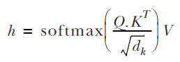
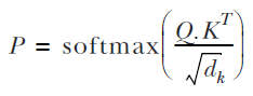
Here, the component  (which will be referred to as P) is a probability matrix. This is all there is in the self-attention layer. Implementing self-attention with TensorFlow is very straightforward. As good data scientists, let’s create it as a reusable Keras layer, as shown in the next listing.
Listing 5.1 The self-attention sublayer
import tensorflow as tf
import tensorflow.keras.layers as layers

class SelfAttentionLayer(layers.Layer):

    def __init__(self, d):
        super(SelfAttentionLayer, self).__init__()
        self.d = d                                                                ❶

    def build(self, input_shape):
        self.Wq = self.add_weight(                                                ❷
            shape=(input_shape[-1], self.d), initializer='glorot_uniform',        ❷
            trainable=True, dtype='float32'                                       ❷
        )
        self.Wk = self.add_weight(                                                ❷
            shape=(input_shape[-1], self.d), initializer='glorot_uniform',        ❷
            trainable=True, dtype='float32'                                       ❷
        )
        self.Wv = self.add_weight(                                                ❷
            shape=(input_shape[-1], self.d), initializer='glorot_uniform',        ❷
            trainable=True, dtype='float32'                                       ❷
        )

    def call(self, q_x, k_x, v_x):
        q = tf.matmul(q_x,self.Wq)                                                ❸
        k = tf.matmul(k_x,self.Wk)                                                ❸
        v = tf.matmul(v_x,self.Wv)                                                ❸

        p = tf.nn.softmax(tf.matmul(q, k, transpose_b=True)/math.sqrt(self.d))    ❹
        h = tf.matmul(p, v)                                                       ❺
        return h,p
❶ Defining the output dimensionality of the self-attention outputs
❷ Defining the variables for computing the query, key, and value entities
❸ Computing the query, key, and value tensors
❹ Computing the probability matrix
-
build(self, input_shape)—Creates the parameters of the layer as variables
-
call(self, v_x, k_x, q_x)—Defines the computations happening in the layer
If you look at the call(self, v_x, k_x, q_x) function, it takes in three inputs: one each for computing value, key, and query. In most cases these are the same input. However, there are instances where different inputs come into these computations (e.g., some computations in the decoder). Also, note that we return both h (i.e., the final output) and p (i.e., the probability matrix). The probability matrix is an important visual aid, as it helps us understand when and where the model paid attention to words. If you want to get the output of the layer, you can do the following
layer = SelfAttentionLayer(512)
h, p = layer(x, x, x)
print(h.shape)
>>> (1, 7, 512)
x = tf.constant(np.random.normal(size=(1,10,256)))
and assuming we need an output of size 512, write the code to create Wq, Wk, and Wv as tf.Variable objects. Use the np.random.normal() function to set the initial values.
5.2.4 Understanding self-attention using scalars
It is not yet very clear why the computations are designed the way they are. To understand and visualize what this layer is doing, we will assume a feature dimensionality of 1. That is, a single word is represented by a single value (i.e., a scalar). Figure 5.6 visualizes the computations that happen in the self-attention layer if we assume a single-input sequence and the dimensionality of inputs (dmodel), query length (dq), key length (dk), and value length (dv) is 1. As a concrete example, we start with an input sequence x, which has seven words (i.e., n × 1 matrix). Under the assumptions we’ve made, Wq, Wk, and Wv will be scalars. The matrix multiplications used for computing q, k, and v essentially become scalar multiplications:
q = (q1, q2,..., q7), where qi = xi Wq
k = (k1, k2,..., k7), where ki = xi Wk
v = (v1, v2,..., v7), where vi = xi Wv
Next, we need to compute the P = softmax ((Q.KT) / √(dk)) component. Q.KT is essentially an n × n matrix that has an item representing every query and key combination (figure 5.6). The i th row and j th column of Q.K(i,j)T are computed as
Then, by applying the softmax, this matrix is converted to a row-wise probability distribution. You might have noted a constant √(dk) appearing within the softmax transformation. This is a normalization constant that helps prevent large gradient values and achieve stable gradients. In our example, you can ignore this as √(dk) = 1.
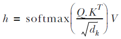
Finally, we compute the final output h = (h1,h2,...,h7), where
hi = P(i,1) v1 + P(i,2) v2 +...+ P(i,7) v7
Here, we can more clearly see the relationship between q, k, and v. q and k are used to compute a soft-index mechanism for v when computing the final output. For example, when computing the fourth output (i.e., h4), we first hard-index the fourth row (following q4), and then mix various v values based on the soft index (i.e., probabilities) given by the columns (i.e., k values) of that row. Now it is more clear what purpose q, k, and v serve:
-
Query—Helps build a probability matrix that is eventually used for indexing values (v). Query affects the rows of the matrix and represents the index of the current word that’s being processed.
-
Key—Helps build a probability matrix that is eventually used for indexing values (v). Key affects the columns of the matrix and represents the candidate words that need to be mixed depending on the query word.
-
Value—Hidden (i.e., attended) representation of the inputs used to compute the final output by indexing using the probability matrix created using query and key
You can easily take the big gray box in figure 5.6, place it over the self-attention sublayer, and still have the output shape (as shown in figure 5.5) being produced (figure 5.7).

Figure 5.6 The computations in the self-attention layer. The self-attention layer starts with an input sequence and computes sequences of query, key, and value vectors. Then the queries and keys are converted to a probability matrix, which is used to compute the weighted sum of values.

Figure 5.7 (top) and figure 5.6 (bottom). You can take the gray box from the bottom and plug it into a self-attention sublayer on the top and see that the same output sequence is being produced.
Now let’s scale up our self-attention layer and revisit the specific computations behind it and why they matter. Going back to our previous notation, we start with a sequence of words, which has n elements. Then, after the embedding lookup, which retrieves an embedding vector for each word, we have a matrix of size n × dmodel. Next, we have the weights and biases to compute each of the query, key, and value vectors:
q = xWq, where x ∈ ℝn×dmodel. Wq ∈ ℝdmodel×dq and q ∈ ℝn×dq
k = xWk, where x ∈ ℝn×dmodel. Wk ∈ ℝdmodel×dk and k ∈ ℝn×dk
v = xWv, where x ∈ ℝn×dmodel. Wv ∈ ℝdmodel×dv and v ∈ ℝn×dv
For example, the query, or q, is a vector of size n × dq, obtained by multiplying the input x of size n × dmodel with the weight matrix Wq of size dmodel × dq. Also remember that, as in the original Transformer paper, we make sure that all of the input embedding of query, key, and value vectors are the same size. In other words,
Next, we compute the probability matrix using the q and k values we obtained:
Finally, we multiply this probably matrix with our value matrix to obtain the final output of the self-attention layer:
The self-attention layer takes a batch of a sequence of words (e.g., a batch of sentences of fixed length), where each word is represented by a vector, and produces a batch of a sequence of hidden outputs, where each hidden output is a vector.
5.2.5 Self-attention as a cooking competition
The concept of self-attention might still be a little bit elusive, making it difficult to understand what exactly is transpiring in the self-attention sublayer. The following analogy might alleviate the burden and make it easier. Say you are taking part in a cooking show with six other contestants (seven contestants in total). The game is as follows.
You are at a supermarket and are given a T-shirt with a number on it (from 1-7) and a trolley. The supermarket has seven aisles. You have to sprint to the aisle with the number on your T-shirt, and there will be a name of some beverage (e.g., apple juice, orange juice, lime juice) posted on the wall. You need to pick what’s necessary to make that beverage, sprint to your allocated table, and make that beverage.
Say that you are number 4 and got orange juice, so you’ll make your way to aisle 4 and collect oranges, a bit of salt, a lime, sugar, and so on. Now say the opponent next to you (number 3), had to make lime juice; they will pick limes, sugar, and salt. As you can see, you are picking different items as well as different quantities of the same item. For example, your opponent hasn’t picked oranges, but you have, and you probably picked fewer limes compared to your opponent who is making lime juice.
This is quite similar to what’s happening in the self-attention layer. You and your contestants are the inputs (at a single time step) to the model. The aisles are the queries, and the grocery items you have to pick are the keys. Just like indexing the probability matrix with query and keys to get the “mixing coefficients” (i.e., attention weights) for the values, you index the items you need by the aisle number allocated to you (i.e., query) and the quantity of each item in the aisle (i.e., key). Finally, the beverage you make is the value. Note that this analogy does not have 100% correspondence to the computations in the self-attention sublayer. However, you can draw significant similarities between the two processes at an abstract level. The similarities we discovered are shown in figure 5.8.
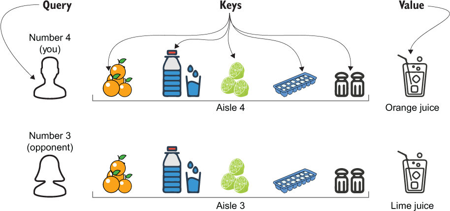
Figure 5.8 Self-attention depicted with the help of a cooking competition. The contestants are the queries, the keys are the grocery items you have to choose from, and the values are the final beverage you’re making.
Next we will discuss what is meant by a masked self-attention layer.
5.2.6 Masked self-attention layers
As you have already seen, the decoder has a special additional self-attention sublayer called masked self-attention. As we have already stated, the idea is to prevent the model from “cheating” by attending to the words it shouldn’t (i.e., the words ahead of the position the model has predicted for). To understand this better, assume two people are teaching a student to translate from English to French. The first person gives an English sentence, asks the student to produce the translation word by word, and provides feedback up to the word translated so far. The second person gives an English sentence and asks the student to produce the translation but provides the full translation in advance. In the second instance, it is much easier for a student to cheat, providing a good quality translation, while having very little knowledge of the languages. Now let’s understand the looming danger of attending to the words it shouldn’t from a machine learning point of view.
Take the task of translating the sentence “dogs are great” to “les chiens sont super.” When processing the sentence “Dogs are great,” the model should be able to attend to any word in that sentence, as that’s an input fully available to the model at any given time. But, while processing the sentence “Les chiens sont super,” we need to be careful about what we show to the model and what we don’t. For example, while training the model, we typically feed the full output sequence at once, as opposed to iteratively feeding the words, to enhance computational efficiency. When feeding the full output sequence to the decoder, we must mask all words ahead of what is currently being processed because it is not fair for the model to predict the word “chiens” when it can see everything that comes after that word. It is imperative you do this. If you don’t, the code will run fine. But ultimately you will have very poor performance when you bring it to the real world. The way to force this is by making the probability matrix p a lower-triangular matrix. This will essentially give zero probability for mixing any input ahead of itself during the attention/output computation. The differences between standard self-attention and masked self-attention are shown in figure 5.9.

Figure 5.9 Standard self-attention versus masked self-attention methods. In the standard attention method, a given step can see an input from any other timestep, regardless of whether those inputs appear before or after the current time step. However, in the masked self-attention method, the current timestep can only see the current input and what came before that time step.
Let’s learn how we can do this in TensorFlow. We do a very simple change to the call() function by introducing a new argument, mask, which represents the items the model shouldn’t see with a 1 and the rest with a 0. Then, to those elements the model shouldn’t see, we add a very large negative number (i.e., - 109) so that when softmax is applied they become zeros (listing 5.2).
Listing 5.2 Masked self-attention sublayer
import tensorflow as tf

class SelfAttentionLayer(layers.Layer):

    def __init__(self, d):
        ...

    def build(self, input_shape):
        ...

    def call(self, q_x, k_x, v_x, mask=None):   ❶
        q = tf.matmul(x,self.Wq)
        k = tf.matmul(x,self.Wk)
        v = tf.matmul(x,self.Wv)

        p = tf.matmul(q, k, transpose_b=True)/math.sqrt(self.d)
        p = tf.squeeze(p)
        if mask is None:
            p = tf.nn.softmax(p)                ❷
        else:
            p += mask * -1e9                    ❸
            p = tf.nn.softmax(p)                ❸


        h = tf.matmul(p, v)
        return h,p
❶ The call function takes an additional mask argument (i.e., a matrix of 0s and 1s).
❷ Now, the SelfAttentionLayer supports both masked and unmasked inputs.
❸ If the mask is provided, add a large negative value to make the final probabilities zero for the words not to be seen.
Creating the mask is easy; you can use the tf.linalg.band_part() function to create triangular matrices
mask = 1 - tf.linalg.band_part(tf.ones((7, 7)), -1, 0)
>>> tf.Tensor(
    [[0. 1. 1. 1. 1. 1. 1.]
     [0. 0. 1. 1. 1. 1. 1.]
     [0. 0. 0. 1. 1. 1. 1.]
     [0. 0. 0. 0. 1. 1. 1.]
     [0. 0. 0. 0. 0. 1. 1.]
     [0. 0. 0. 0. 0. 0. 1.]
     [0. 0. 0. 0. 0. 0. 0.]], shape=(7, 7), dtype=float32)
We can easily verify if the masking worked by looking at the probability matrix p. It must be a lower triangular matrix
layer = SelfAttentionLayer(512)
h, p = layer(x, x, x, mask)
print(p.numpy())
>>> [[1.    0.    0.    0.    0.    0.    0.   ]
     [0.37  0.63  0.    0.    0.    0.    0.   ]
     [0.051 0.764 0.185 0.    0.    0.    0.   ]
     [0.138 0.263 0.072 0.526 0.    0.    0.   ]
     [0.298 0.099 0.201 0.11  0.293 0.    0.   ]
     [0.18  0.344 0.087 0.25  0.029 0.108 0.   ]
     [0.044 0.044 0.125 0.284 0.351 0.106 0.045]]
Now, when computing the value, the model cannot see or attend the words it hasn’t seen by the time it comes to the current word.
5.2.7 Multi-head attention
The original Transformer paper discusses something called multi-head attention, which is an extension of the self-attention layer. The idea is simple once you understand the self-attention mechanism. The multi-head attention creates multiple parallel self-attention heads. The motivation for this is that, practically, when the model is given the opportunity to learn multiple attention patterns (i.e., multiple sets of weights) for an input sequence, it performs better.
Remember that in a single attention head we had all query, key, and value dimensionality set to 512. In other words,
With multi-head attention, assuming we are using eight attention heads,
Then the final outputs of all attention heads are concatenated to create the final output, which will have a dimensionality of 64 × 8 = 512
where hi is the output of the ith attention head. Using the SelfAttentionLayer we just implemented, the code becomes
multi_attn_head = [SelfAttentionLayer(64) for i in range(8)]
outputs = [head(x, x, x)[0] for head in multi_attn_head]
outputs = tf.concat(outputs, axis=-1)
print(outputs.shape)
>>> (1, 7, 512)
As you can see, it still has the same shape as before (without multiple heads). However, this output is computed using multiple heads, which have smaller dimensionality than the original self-attention layer.
5.2.8 Fully connected layer
The fully connected layer is a piece of cake compared to what we just learned. So far, the self-attention layer has produced a n × dv-sized output (ignoring the batch dimension). The fully connected layer takes this input and performs the following transformation
where W1 is a dv × dff1 matrix and b1 is a dff1-sized vector. Therefore, this operation gives out a n×dff1-sized tensor. The resulting output is passed onto another layer, which does the following computation
where W2 is a dff1 × dff2-sized matrix and b2 is a dff2-sized vector. This operation gives a tensor of size n × dff2. In TensorFlow parlance, we can again encapsulate these computations as a reusable Keras layer (see the next listing).
Listing 5.3 The fully connected sublayer
import tensorflow as tf

class FCLayer(layers.Layer):
    def __init__(self, d1, d2):
        super(FCLayer, self).__init__()
        self.d1 = d1                                                       ❶
        self.d2 = d2                                                       ❷

    def build(self, input_shape):
        self.W1 = self.add_weight(                                         ❸
            shape=(input_shape[-1], self.d1), initializer='glorot_uniform',❸
            trainable=True, dtype='float32'                                ❸
        )
        self.b1 = self.add_weight(                                         ❸
            shape=(self.d1,), initializer='glorot_uniform',                ❸
            trainable=True, dtype='float32'                                ❸
        )
        self.W2 = self.add_weight(                                         ❸
            shape=(input_shape[-1], self.d2), initializer='glorot_uniform',❸
            trainable=True, dtype='float32'                                ❸
        )
        self.b2 = self.add_weight(                                         ❸
            shape=(self.d2,), initializer='glorot_uniform',                ❸
            trainable=True, dtype='float32'                                ❸
        )

    def call(self, x):
        ff1 = tf.nn.relu(tf.matmul(x,self.W1)+self.b1)                     ❹
        ff2 = tf.matmul(ff1,self.W2)+self.b2                               ❺
        return ff2
❶ The output dimensionality of the first fully connected computation
❷ The output dimensionality of the second fully connected computation
❸ Defining W1, b1, W2, and b2 accordingly. We use glorot_uniform as the initializer.
❹ Computing the first fully connected computation
❺ Computing the second fully connected computation
Here, you could use the tensorflow.keras.layers.Dense() layer to implement this functionality. However, we will do it with raw TensorFlow operations as an exercise to familiarize ourselves with low-level TensorFlow. In this setup, we will change the FCLayer, as shown in the following listing.
Listing 5.4 The fully connected layer implemented using Keras Dense layers
import tensorflow as tf
import tensorflow.keras.layers as layers

class FCLayer(layers.Layer):

    def __init__(self, d1, d2):
        super(FCLayer, self).__init__()
        self.dense_layer_1 = layer.Dense(d1, activation='relu')  ❶
        self.dense_layer_2 = layers.Dense(d2)                    ❷

    def call(self, x):
        ff1 = self.dense_layer_1(x)                              ❸
        ff2 = self.dense_layer_2(ff1)                            ❹
        return ff2
❶ Defining the first Dense layer in the __init__ function of the subclassed layer
❷ Defining the second Dense layer. Note how we are not specifying an activation function.
❸ Calling the first dense layer to get the output
❹ Calling the second dense layer with the output of the first Dense layer to get the final output
Now you know what computations take place in the Transformer architecture and how to implement them with TensorFlow. But keep in mind that there are various fine-grained details explained in the original Transformer paper, which we haven’t discussed. Most of these details will be discussed in a later chapter.
Say you have been asked to experiment with a new type of multi-head attention mechanism. Instead of concatenating outputs from smaller heads (of size 64), the outputs (of size 512) are summed. Write TensorFlow code using the SelfAttentionLayer to achieve this effect. You can use the tf.math.add_n() function to sum a list of tensors element-wise.
5.2.9 Putting everything together
Let’s bring all these elements together to create a Transformer network. Let’s first create an encoder layer, which contains a set of SelfAttentionLayer objects (one for each head) and a FCLayer (see the next listing).
import tensorflow as tf

class EncoderLayer(layers.Layer):

    def __init__(self, d, n_heads):
        super(EncoderLayer, self).__init__()
        self.d = d
        self.d_head = int(d/n_heads)
        self.n_heads = n_heads
        self.attn_heads = [
            SelfAttentionLayer(self.d_head) for i in range(self.n_heads)
        ]                                           ❶
        self.fc_layer = FCLayer(2048, self.d)       ❷

    def call(self, x):
        def compute_multihead_output(x):            ❸
            outputs = [head(x, x, x)[0] for head in self.attn_heads]
            outputs = tf.concat(outputs, axis=-1)
            return outputs

        h1 = compute_multihead_output(x)            ❹
        y = self.fc_layer(h1)                       ❺

        return y
❶ Create multiple attention heads. Each attention head has d/n_heads-sized feature dimensionality.
❷ Create the fully connected layer, where the intermediate layer has 2,048 nodes and the final sublayer has d nodes.
❸ Create a function that computes the multi-head attention output given an input.
❹ Compute multi-head attention using the defined function.
❺ Get the final output of the layer.
The EncoderLayer takes in two parameters during initialization: d (dimensionality of the output) and n_heads (number of attention heads). Then, when calling the layer, a single input x is passed. First, the attended output of the attention heads (SelfAttentionLayer) is computed, followed by the output of the fully connected layer (FCLayer). This wraps the crux of an encoder layer. Next, we create a Decoder layer (see the next listing).
import tensorflow as tf

class DecoderLayer(layers.Layer):

    def __init__(self, d, n_heads):
        super(DecoderLayer, self).__init__()
        self.d = d
        self.d_head = int(d/n_heads)
        self.dec_attn_heads = [
            SelfAttentionLayer(self.d_head) for i in range(n_heads)
        ]                                                           ❶
        self.attn_heads = [
            SelfAttentionLayer(self.d_head) for i in range(n_heads)
        ]                                                           ❷
        self.fc_layer = FCLayer(2048, self.d)                       ❸

    def call(self, de_x, en_x, mask=None):
        def compute_multihead_output(de_x, en_x, mask=None):        ❹
            outputs = [
                head(en_x, en_x, de_x, mask)[0] for head in
➥ self.attn_heads]                                                 ❺
            outputs = tf.concat(outputs, axis=-1)
            return outputs

        h1 = compute_multihead_output(de_x, de_x, mask)             ❻
        h2 = compute_multihead_output(h1, en_x)                     ❼
        y = self.fc_layer(h2)                                       ❽
        return y
❶ Create the attention heads that process the decoder input only.
❷ Create the attention heads that process both the encoder output and decoder input.
❸ The final fully connected sublayer
❹ The function that computes the multi-head attention. This function takes three inputs (decoder’s previous output, encoder output, and an optional mask).
❺ Each head takes the first argument of the function as the query and key and the second argument of the function as the value.
❻ Compute the first attended output. This only looks at the decoder inputs.
❼ Compute the second attended output. This looks at both the previous decoder output and the encoder output.
❽ Compute the final output of the layer by feeding the output through a fully connected sublayer.
The decoder layer has several differences compared to the encoder layer. It contains two multi-head attention layers (one masked and one unmasked) and a fully connected layer. First, the output of the first multi-head attention layer (masked) is computed. Remember that we are masking any decoder input that is ahead of the current decoder input that’s been processed. We use the decoder inputs to compute the output of the first attention layer. However, the computations happening in the second layer are a bit tricky. Brace yourselves! The second attention layer takes the encoder network’s last attended output as query and key; then, to compute the value, the output of the first attention layer is used. Think of this layer as a mixer that mixes attended encoder outputs and attended decoder inputs.
With that, we can create a simple Transformer model with two encoder layers and two decoder layers). We’ll use the Keras functional API (see the next listing).
Listing 5.7 The full Transformer model
import tensorflow as tf

n_steps = 25                                                              ❶
n_en_vocab = 300                                                          ❶
n_de_vocab = 400                                                          ❶
n_heads = 8                                                               ❶
d = 512                                                                   ❶
mask = 1 - tf.linalg.band_part(tf.ones((n_steps, n_steps)), -1, 0)        ❷

en_inp = layers.Input(shape=(n_steps,))                                   ❸
en_emb = layers.Embedding(n_en_vocab, 512, input_length=n_steps)(en_inp)  ❹
en_out1 = EncoderLayer(d, n_heads)(en_emb)                                ❺
en_out2 = EncoderLayer(d, n_heads)(en_out1)

de_inp = layers.Input(shape=(n_steps,))                                   ❻
de_emb = layers.Embedding(n_de_vocab, 512, input_length=n_steps)(de_inp)  ❼
de_out1 = DecoderLayer(d, n_heads)(de_emb, en_out2, mask)                 ❽
de_out2 = DecoderLayer(d, n_heads)(de_out1, en_out2, mask)
de_pred = layers.Dense(n_de_vocab, activation='softmax')(de_out2)         ❾

transformer = models.Model(
    inputs=[en_inp, de_inp], outputs=de_pred, name='MinTransformer'       ❿
)
transformer.compile(
    loss='categorical_crossentropy', optimizer='adam', metrics=['acc']
)
❶ The hyperparameters of the Transformer model
❷ The mask that will be used to mask decoder inputs
❸ The encoder’s input layer. It accepts a batch of a sequence of word IDs.
❹ The embedding layer that will look up the word ID and return an embedding vector for that ID
❺ Compute the output of the first encoder layer.
❻ The decoder’s input layer. It accepts a batch of a sequence of word IDs.
❼ The decoder’s embedding layer
❽ Compute the output of the first decoder layer.
❾ The final prediction layer that predicts the correct output sequence
❿ Defining the model. Note how we are providing a name for the model.
Before diving into the details, let’s refresh our memory with what the Transformer architecture looks like (figure 5.10).

Figure 5.10 The Transformer model architecture
Since we have explored the underpinning elements quite intensively, the network should be very easy to follow. All we have to do is set up the encoder model, set up the decoder model, and combine these appropriately by creating a Model object. Initially we define several hyperparameters. Our model takes n_steps-long sentences. This means that if a given sentence is shorter than n_steps, we will pad a special token to make it n_steps long. If a given sentence is longer than n_steps, we will truncate the sentence up to n_steps words. The larger the n_steps value, the more information you retain in the sentences, but also the more memory your model will consume. Next, we have the vocabulary size of the encoder inputs (i.e., the number of unique words in the data set fed to the encoder) (n_en_vocab), the vocabulary size of the decoder inputs (n_de_vocab), the number of heads (n_heads), and the output dimensionality (d).
With that we have defined the encoder input layer, which takes a batch of n_steps-long sentences. In these sentences, each word will be represented by a unique ID. For example, the sentence “The cat sat on the mat” will be converted to [1, 2, 3, 4, 1, 5]. Next, we have a special layer called Embedding, which provides a d elements-long representation for each word (i.e., word vectors). After this transformation, you have a (batch size, n_steps, d)-sized output, which is the format of the output that should go into the self-attention layer. We discussed this transformation briefly in chapter 3 (section 3.4.3). The Embedding layer is essentially a lookup table. Given a unique ID (each ID represents a word), it gives out a vector that is d elements long. In other words, this layer encapsulates a large matrix of size (vocabulary size, d). You can see that when defining the Embedding layer:
layers.Embedding(n_en_vocab, 512, input_length=n_steps)
We need to provide the vocabulary size (the first argument) and the output dimensionality (the second argument), and finally, since we are processing an input sequence of length n_steps, we need to specify the input_length argument. With that, we can pass the output of the embedding layer (en_emb) to an Encoder layer. You can see that we have two encoder layers in our model.
Next, moving on to the decoder, everything at a high level looks identical to the encoder, except for two differences:
-
The Decoder layer takes both the encoder output (en_out2) and the decoder input (de_emb or de_out1) as inputs.
-
The Decoder layer also has a final Dense layer that produces the correct output sequence (e.g., in a machine translation task, these would be the translated word probabilities for each time step).
You can now define and compile the model as
transformer = models.Model(
    inputs=[en_inp, de_inp], outputs=de_pred, name=’MinTransformer’
)
transformer.compile(
    loss='categorical_crossentropy', optimizer='adam', metrics=['acc']
)
Note that we can provide a name for our model when defining it. We will name our model “MinTransformer.” As the final step, let’s look at the model summary,
transformer.summary()
which will provide the following output:
Model: "MinTransformer"
_____________________________________________________________________________________________
Layer (type)                    Output Shape         Param #     Connected to
=============================================================================================
input_1 (InputLayer)            [(None, 25)]         0
_____________________________________________________________________________________________
embedding (Embedding)           (None, 25, 512)      153600      input_1[0][0]
_____________________________________________________________________________________________
input_2 (InputLayer)            [(None, 25)]         0
_____________________________________________________________________________________________
encoder_layer (EncoderLayer)    (None, 25, 512)      2886144     embedding[0][0]
_____________________________________________________________________________________________
embedding_1 (Embedding)         (None, 25, 512)      204800      input_2[0][0]
_____________________________________________________________________________________________
encoder_layer_1 (EncoderLayer)  (None, 25, 512)      2886144     encoder_layer[0][0]
_____________________________________________________________________________________________
decoder_layer (DecoderLayer)    (None, 25, 512)      3672576     embedding_1[0][0]
                                                                 encoder_layer_1[0][0]
_____________________________________________________________________________________________
decoder_layer_1 (DecoderLayer)  (None, 25, 512)      3672576     decoder_layer[0][0]
                                                                 encoder_layer_1[0][0]
_____________________________________________________________________________________________
dense (Dense)                   (None, 25, 400)      205200      decoder_layer_1[0][0]
=============================================================================================
Total params: 13,681,040
Trainable params: 13,681,040
Non-trainable params: 0
_____________________________________________________________________________________________
The workshop participants are going to walk out of this workshop a happy bunch. You have covered the essentials of Transformer networks while teaching the participants to implement their own. We first explained that the Transformer has an encoder-decoder architecture. We then looked at the composition of the encoder and the decoder, which are made of self-attention layers and fully connected layers. The self-attention layer allows the model to attend to other input words while processing a given input word, which is important when processing natural language. We also saw that, in practice, the model uses multiple attention heads in a single attention layer to improve performance. Next, the fully connected layer creates a nonlinear representation of the attended output. After understanding the basic elements, we implemented a basic small-scale Transformer network using reusable custom layers we created for the self-attention (SelfAttentionLayer) and fully connected layer (FCLayer).
The next step is to train this model on an NLP data set (e.g., machine translation). However, training these models is a topic for a separate chapter. There’s a lot more to Transformers than what we have discussed. For example, there are pretrained transformer-based models that you can use readily to solve NLP tasks. We will revisit Transformers again in a later chapter.
Summary
-
Transformer networks have outperformed other models in almost all NLP tasks.
-
Transformers are an encoder-decoder-type neural network that is mainly used for learning NLP tasks.
-
With Transformers, the encoder and decoder are made of two computational sublayers: self-attention layers and fully connected layers.
-
The self-attention layer produces a weighted sum of inputs for a given time step, based on how important it is to attend to other positions in the sequence while processing the current position.
-
The fully connected layer creates a nonlinear representation of the attended output produced by the self-attention layer.
-
The decoder uses masking in its self-attention layer to make sure that the decoder does not see any future predictions while producing the current prediction.
Answers to exercises
Wq = tf.Variable(np.random.normal(size=(256,512)))
Wk = tf.Variable (np.random.normal(size=(256,512)))
Wv = tf.Variable (np.random.normal(size=(256,512)))
multi_attn_head = [SelfAttentionLayer(512) for i in range(8)]
outputs = [head(x)[0] for head in multi_attn_head]
outputs = tf.math.add_n(outputs)