15 TFX: MLOps and deploying models with TensorFlow

This chapter covers

• Writing an end-to-end data pipeline using TFX (TensorFlow-Extended)
• Training a simple neural network through the TFX Trainer API
• Using Docker to containerize model serving (inference) and present it as a service
• Deploying the model on your local machine so it can be used through an API

In chapter 14, we looked at a very versatile tool that comes with TensorFlow: the TensorBoard. TensorBoard is a visualization tool that helps you understand data and models better. Among other things, it facilitates

• Monitoring and tracking model performance

• Visualizing data inputs to models (e.g., images, audio)

• Profiling models to understand their performance or memory bottlenecks

We learned how we can use the TensorBoard to visualize high-dimensional data like images and word vectors. We looked at how we can incorporate Keras callbacks to send information to the TensorBoard to visualize model performance (accuracy and loss) and custom metrics. We then analyzed the execution of the model using the CUDA profiling tool kit to understand execution patterns and memory bottlenecks.

In this chapter, we will explore a new domain of machine learning that has gained an enormous amount of attention in the recent past: MLOps. MLOps is derived from the terms ML and DevOps (derived from development and operations). According to Amazon Web Services, “DevOps is the combination of cultural philosophies, practices, and tools that increases an organization’s ability to deliver applications and services at high velocity: evolving and improving products at a faster pace than organizations using traditional software development and infrastructure management processes.” There is another term that goes hand in hand with MLOps, which is productionization of models. It is somewhat difficult to discriminate between the two terms as they overlap and occasionally are used interchangeably, but I like to think of these two things as follows: MLOps defines a workflow that will automate most of the steps, from collecting data to delivering a model trained on that data, with very little human intervention. Productionization is deploying a trained model (on a private server or cloud), enabling customers to use the model for its designed purpose in a robust fashion. It can include tasks such as designing scalable APIs that can scale to serve thousands of requests per second. In other words, MLOps is the journey that gets you to the destination, which is the productionization of a model.

Let’s discuss why it is important to have a (mostly) automated pipeline to develop machine learning models. To realize the value of it, you have to think in scale. For companies like Google, Facebook, and Amazon, machine learning is deeply rooted in the products they offer. This means hundreds if not thousands of models produce predictions every second. Moreover, with a few billion users, they can’t afford their models to go stale, which means continuously training/fine-tuning the existing models as new data is collected. MLOps can take care of this problem. MLOps can be used to ingest the collected data, train models, automatically evaluate models, and push them to the production environment if they pass a predefined validation check. A validation check is important to ensure models meet expected performance standards and to safeguard against rogue underperforming models (e.g., a rogue model can be generated due to large changes in new incoming training data, a new untested hyperparameter change that is pushed, etc.). Finally, the model is pushed to a production environment, which is accessed through a Web API to retrieve predictions for an input. Specifically, the API will provide certain endpoints (in the form of URLs) to the user that the user can visit (optionally with parameters needed to complete the request). Having said that, even for a smaller company that is relying on machine learning models, MLOps can greatly standardize and speed up the workflows of data scientists and machine learning engineers. This will greatly reduce the time data scientists and machine learning engineers spend creating such workflows from the ground up every time they work on a new project. Read more about MLOps at http://mng.bz/Pnd9.

How can we do MLOps in TensorFlow? Look no further than TFX (TensorFlow Extended). TFX is a library that gives you all the bells and whistles needed to implement a machine learning pipeline that will ingest data, transform data into features, train a model, and push the model to a designated production environment. This is done by defining a series of components that perform very specific tasks. In the coming sections, we will look at how to use TFX to achieve this.

15.1 Writing a data pipeline with TFX

Imagine you are developing a system to predict the severity of a forest fire given the weather conditions. You have been given a data set from past observed forest fires and asked to make a model. To make sure you can provide the model as a service, you decide to create a workflow to ingest data and train a model using TFX. The first step in this is to create a data pipeline that can read the data (in CSV format) and convert it to features. As part of this pipeline, you will have a data reader (that generates examples from CSV), show summary statistics of the fields, learn the schema of the data, and convert it to a proper format the model understands.

The first thing to do is download the data sets (listing 15.1). We will use a data set that has recorded historical forest fires in the Montesinho park in Portugal. The data set is freely available at http://archive.ics.uci.edu/ml/datasets/Forest+Fires. It is is a CSV file with the following features:

• X—x-axis spatial coordinate within the Montesinho park map

• Y—y-axis spatial coordinate within the Montesinho park map

• month—Month of the year

• day—Day of the week

• Fine Fuel Moisture Code (FFMC)—Represents fuel moisture of forest litter fuels under the shade of a forest canopy

• DMC—A numerical rating of the average moisture content of soil

• Drought Code (DC)—Represents the depth of dryness in the soil

• Initial Spread Index (ISI)—An expected rate of fire spread

• temp—Temperature in Celsius degrees

• RH—Relative humidity in %

• wind—Wind speed in km/h

• rain—Outside rain in mm/m2

• area—The burnt area of the forest (in hectares)

Our task will be to predict the burnt area, given all the other features. Note that predicting a continuous value such as the area warrants a regression model. Therefore, this is a regression problem, not a classification problem.

Listing 15.1 Downloading the data set

import os
import requests
import tarfile
 
import shutil
 
if not os.path.exists(os.path.join('data', 'csv', 'forestfires.csv')):    ❶
    url = "http:/ /archive.ics.uci.edu/ml/machine-learning-databases/forest-
➥ fires/forestfires.csv"
    r = requests.get(url)                                                 ❷
 
    if not os.path.exists(os.path.join('data', 'csv')):                   ❸
        os.makedirs(os.path.join('data', 'csv'))                          ❸
    
    with open(os.path.join('data', 'csv', 'forestfires.csv'), 'wb') as f: ❸
        f.write(r.content)                                                ❸
else:
    print("The forestfires.csv file already exists.")
    
  
if not os.path.exists(os.path.join('data', 'forestfires.names')):         ❹
    
    url = "http:/ /archive.ics.uci.edu/ml/machine-learning-databases/forest-
➥ fires/forestfires.names"
    r = requests.get(url)                                                 ❹
 
    if not os.path.exists('data'):                                        ❺
        os.makedirs('data')                                               ❺
    
    with open(os.path.join('data', 'forestfires.names'), 'wb') as f:      ❺
        f.write(r.content)                                                ❺
        
else:
    print("The forestfires.names file already exists.")

❶ If the data file is not downloaded, download the file.

❷ This line downloads a file given by a URL.

❸ Create the necessary folders and write the downloaded data into it.

❹ If the file containing the data set description is not downloaded, download it.

❺ Create the necessary directories and write the data into them.

Here, we download two files: forestfires.csv and forestfires.names. forestfires.csv contains the data in a comma-separated format, where the first line is the header followed by data in the rest of the file. forestfires.names contains more information about the data, in case you want to understand more about it. Next, we will separate a small test data set to do manual testing on later. Having a dedicated test set that is not seen by the model at any stage will tell us how well the model has generalized. This will be 5% of the original data set. The other 95% will be left for training and validation data:

import pandas as pd
 
df = pd.read_csv(
    os.path.join('data', 'csv', 'forestfires.csv'), index_col=None, 
➥ header=0
)
train_df = df.sample(frac=0.95, random_state=random_seed)
test_df = df.loc[~df.index.isin(train_df.index), :]
 
train_path = os.path.join('data','csv','train')
os.makedirs(train_path, exist_ok=True)
test_path = os.path.join('data','csv','test')
os.makedirs(test_path, exist_ok=True)
 
train_df.to_csv(
    os.path.join(train_path, 'forestfires.csv'), index=False, header=True
)
test_df.to_csv(
    os.path.join(test_path, 'forestfires.csv'), index=False, header=True
)

We will now start with the TFX pipeline. The first step is to define a root directory for storing pipeline artifacts. What are pipeline artifacts, you might ask? When running the TFX pipeline, it stores interim results of various stages in a directory (under a certain subdirectory structure). One example of this is that when you read the data from the CSV file, the TFX pipeline will split the data into train and validation subsets, convert those examples to TFRecord objects (i.e., an object type used by TensorFlow internally for data), and store the data as compressed files:

_pipeline_root = os.path.join(
    os.getcwd(), 'pipeline', 'examples', 'forest_fires_pipeline'
)

TFX uses Abseil for logging purposes. Abseil is an open-source collection of C++ libraries drawn from Google’s internal codebase. It provides facilities for logging, command-line argument parsing, and so forth. If you are interested, read more about the library at https://abseil.io/docs/python/. We will set the logging level to INFO so that we will see logging statements at the INFO level or higher. Logging is an important functionality to have, as we can glean lots of insights, including what steps ran successfully and what errors were thrown:

absl.logging.set_verbosity(absl.logging.INFO)

After the initial housekeeping, we will define an InteractiveContext:

from tfx.orchestration.experimental.interactive.interactive_context import 
➥ InteractiveContext
 
context = InteractiveContext(
    pipeline_name = "forest_fires", pipeline_root=_pipeline_root
)

TFX runs pipelines in a context. The context is used to run various steps you define in the pipeline. It also serves a very important purpose, which is to manage states between different steps as we are progressing through the pipeline. In order to manage transitions between states and make sure the pipeline operates as expected, it also maintains a metadata store (a small-scale database). The metadata store contains various information, such as an execution order, the final state of the components, and resulting errors. You can read about metadata in the following sidebar.

We’re off to defining the pipeline. The primary purpose of the pipeline in this section is to

• Load the data from a CSV file and split to training and validation data

• Learn the schema of the data (e.g., various columns, data types, min/max bounds, etc.)

• Display summary statistics and graphs about the distribution of various features

• Transform the raw columns to features, which may require special intermediate processing steps

These steps are a lead-up to model training and deployment. Each of these tasks will be a single component in the pipeline, and we will discuss these in more detail when the time comes.

15.1.1 Loading data from CSV files

The first step is to define a component to read examples from the CSV file and split the data to train and eval. For that, you can use the tfx.components.CsvExampleGen object. All we need to do is provide the directory containing the data to the input_base argument:

from tfx.components import CsvExampleGen
 
example_gen = CsvExampleGen(input_base=os.path.join('data', 'csv', 'train'))

Then we use the previously defined InteractiveContext to run the example generator:

context.run(example_gen)

Let’s look at what this step produces. To see the data, let’s go to the _pipeline_root directory (e.g., Ch15-TFX-for-MLOps-in-TF2/tfx/pipeline). It should have a directory/ file structure similar to what’s shown in figure 15.1.

Figure 15.1 The directory/file structure after running the CsvExampleGen

You will see two GZip files (i.e., with a .gz extension) created within the pipeline. You will notice that there are two sub-directories in the CsvExampleGen folder: Split-train and Split-eval, which contain training and validation data, respectively. When you run the notebook cell containing the previous code, you will also see an output HTML table displaying the inputs and outputs of the TFX component (figure 15.2).

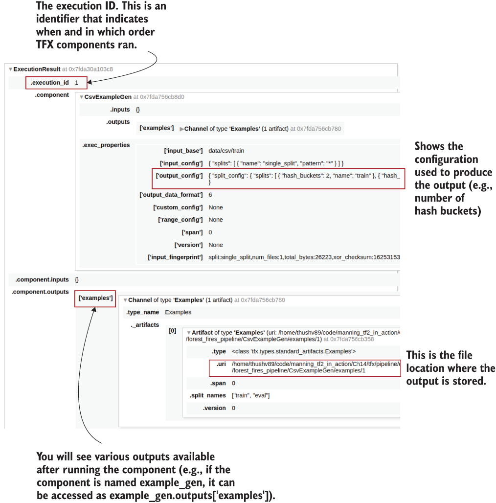
Figure 15.2 Output HTML table generated by running the CsvExampleGen component

There are a few things worth noting. To start, you will see the execution_id, which is the value produced by a counter that keeps track of the number of times you run TFX components. In other words, every time you run a TFX component (like CsvExampleGen), the counter goes up by 1. If you go down further, you can see some important information about how the CsvExampleGen has split your data. If you look under component > CsvExampleGen > exec_properties > output_config, you will see something like

"split_config": { 
    "splits": [ 
        { "hash_buckets": 2, "name": "train" }, 
        { "hash_buckets": 1, "name": "eval" } 
    ] 
} 

This says that the data set has been split into two sets: train and eval. The train set is roughly two-thirds of the original data, and the eval set is around one-third of the original data. This information is inferred by looking at the hash_buckets property. TFX uses hashing to split the data into train and eval. By default, it will define three hash buckets. Then TFX uses the values in each record to generate a hash for that record. The values in the record are passed to a hashing function to generate a hash. The generated hash is then used to assign that example to a bucket. For example, if the hash is 7, then TFX can easily find the bucket with 7%, 3 = 1, meaning it will be assigned to the second bucket (as buckets are zero indexed). You can access the elements in CsvExampleGen as follows.

artifact = example_gen.outputs['examples'].get()[0]
 
print("Artifact split names: {}".format(artifact.split_names))
print("Artifact URI: {}".format(artifact.uri)

This will print the following output:

Artifact split names: ["train", "eval"]
Artifact URI: <path to project>/Ch15-TFX-for-MLOps-in-
➥ TF2/tfx/pipeline/examples/forest_fires_pipeline/CsvExampleGen/examples/1

Earlier we said that TFX stores the interim outputs as we progress through the pipeline. We saw that the CsvExampleGen component has stored the data as .gz files. It in fact stores the examples found in the CSV file as TFRecord objects. A TFRecord is used to store data as byte streams. As TFRecord is a common method for storing data when working with TensorFlow; these records can be retrieved easily as a tf.data.Dataset, and the data can be inspected. The next listing shows how this can be done.

Listing 15.2 Printing the data stored by the CsvExampleGen

train_uri = os.path.join(
    example_gen.outputs['examples'].get()[0].uri, 'Split-train'       ❶
) 
 
tfrecord_filenames = [
    os.path.join(train_uri, name) for name in os.listdir(train_uri)   ❷
]
 
dataset = tf.data.TFRecordDataset(
    tfrecord_filenames, compression_type="GZIP"
)                                                                     ❸
 
for tfrecord in dataset.take(2):                                      ❹
  serialized_example = tfrecord.numpy()                               ❺
  example = tf.train.Example()                                        ❻
  example.ParseFromString(serialized_example)                         ❼
  print(example)                                                      ❽

❶ Get the URL of the output artifact representing the training examples, which is a directory.

❷ Get the list of files in this directory (all compressed TFRecord files).

❸ Create a TFRecordDataset to read these files. The GZip (extension .gz) has a set of TFRecord objects.

❹ Iterate over the first two records (can be any number less than or equal to the size of the data set).

❺ Get the byte stream from the TFRecord (containing one example).

❻ Define a tf.train.Example object that knows how to parse the byte stream.

❼ Parse the byte stream to a proper readable example.

❽ Print the data.

If you run this code, you will see the following:

features {
  feature {
    key: "DC"
    value {
      float_list {
        value: 605.7999877929688
      }
    }
  }
  ...
  feature {
    key: "RH"
    value {
      int64_list {
        value: 43
      }
    }
  }
  feature {
    key: "X"
    value {
      int64_list {
        value: 5
      }
    }
  }
  ...
  feature {
    key: "area"
    value {
      float_list {
        value: 2.0
      }
    }
  }
  feature {
    key: "day"
    value {
      bytes_list {
        value: "tue"
      }
    }
  }
  ...
}
 
...

tf.train.Example keeps the data as a collection of features, where each feature has a key (column descriptor) and a value. You will see all of the features for a given example. For example, the DC feature has a floating value of 605.799, feature RH has an int value of 43, feature area has a floating value of 2.0, and feature day has a bytes_list (used to store strings) value of "tue" (i.e., Tuesday).

Before moving to the next section, let’s remind ourselves what our objective is: to develop a model that can predict the fire spread (in hectares) given all the other features in the data set. This problem is framed as a regression problem.

15.1.2 Generating basic statistics from the data

As the next step, we will understand the data better. This is known as exploratory data analysis (EDA). EDA is not typically well defined and very much depends on the problem you are solving and the data. And you have to factor in the limited time you usually have until the delivery of a project. In other words, you cannot test everything and have to prioritize what you want to test and what you want to assume. For the structured data we are tackling here, a great place to start is understanding type (numerical versus categorical) and the distribution of values of the various columns present. TFX provides you a component just for that. StatisticsGen will automatically generate those statistics for you. We will soon see in more detail what sort of insights this module provides:

from tfx.components import StatisticsGen
 
statistics_gen = StatisticsGen(
    examples=example_gen.outputs['examples'])
 
context.run(statistics_gen)

This will produce an HTML table similar to what you saw after running CsvExampleGen (figure 15.3).

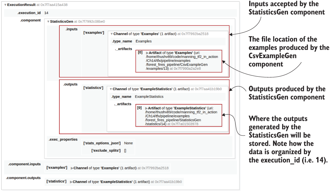
Figure 15.3 The output provided by the StatisticsGen component

However, to retrieve the most valuable output of this step, you have to run the following line:

context.show(statistics_gen.outputs['statistics'])

This will create the following files in the pipeline root (figure 15.4).

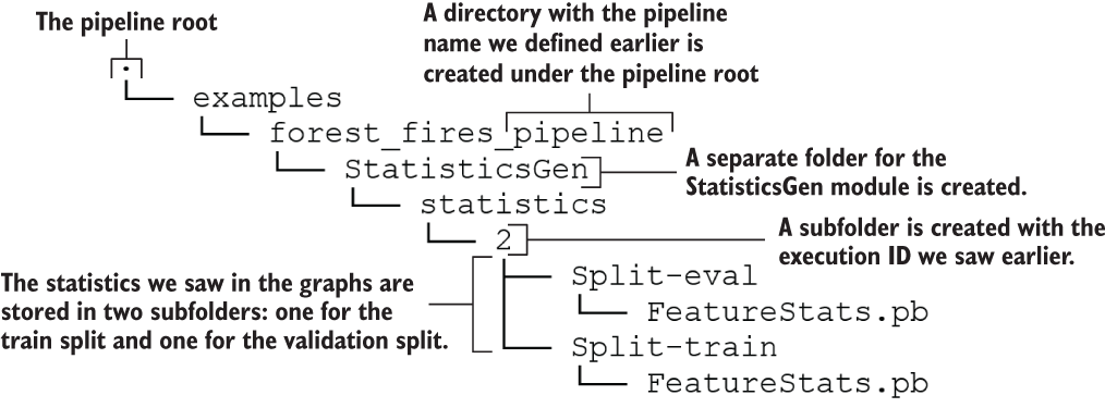
Figure 15.4 The directory/file structure after running StatisticsGen

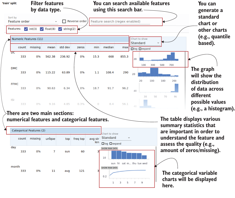
Figure 15.5 shows the valuable collection of information about data provided by TFX. The output graph shown in figure 15.5 is a goldmine containing rich information about the data we’re dealing with. It provides you a basic yet holistic suite of graphs that provides lots of information about the columns present in the data. Let’s go from top to bottom. At the top, you have options to sort and filter the outputs shown in figure 15.5. For example, you can change the order of the graphs, select graphs based on data types, or filter them by a regular expression.

Figure 15.5 The summary statistics graphs generated for the data by the StatisticsGen component

By default, StatisticsGen will generate graphs for both train and eval data sets. Then each train and eval section will have several subsections; in this case, we have a section for numerical columns and categorical columns.

On the left, you can see some numerical statistics and assessments of a feature, whereas on the right side, you can see a visual representation of how a feature is distributed. For example, take the FFMC feature in the training set. We can see that it has 333 examples and 0% have missing values for that feature. It has a mean of ~90 and a standard deviation of 6.34. In the graph, you can see that the distribution is quite skewed. Almost all values are concentrated around the 80-90 range. You will see later how this might create problems for us and how we will solve them.

In the categorical section, you can see the values of the day and month features. For example, the day feature has seven unique values and 0% missing. The most frequent value (i.e., mode) of the day feature appears 60 times. Note that the day is represented as a bar graph and the month is represented as a line graph because for features with unique values above a threshold, a line graph is used to make the graph clear and less cluttered.

15.1.3 Inferring the schema from data

Thus far, we have loaded the data from a CSV file and explored the basic statistics of the data set. The next big step is to infer the schema of the data. TFX can automatically derive the schema of the data once the data is provided. If you have worked with databases, the schema derived is the same as a database schema. It can be thought of as a blueprint for the data, expressing the structure and important attributes of data. It can also be thought of as a set of rules that dictate what the data should look like. For example, if you have the schema, you can classify whether a given record is valid by referring to the schema.

Without further ado, let’s create a SchemaGen object. The SchemaGen requires the output of the previous step (i.e., output of the StatisticsGen) and a Boolean argument named infer_feature_shape:

from tfx.components import SchemaGen
 
schema_gen = SchemaGen(
    statistics=statistics_gen.outputs[‘statistics’],
    infer_feature_shape=False)
 
context.run(schema_gen)

Here, we set the infer_feature_shape to False, as we will do some transformations to the features down the road. Therefore, we will have the flexibility to manipulate the feature shapes more freely. However, setting this argument (infer_feature_shape) means an important change for a downstream step (called the transform step). When infer_feature_shape is set to False, the tensors passed to the transform step are represented as tf.SparseTensor objects, not tf.Tensor objects. If set to True, it will need to be a tf.Tensor object with a known shape. Next, to see the output of the SchemaGen, you can do

context.show(schema_gen.outputs['schema'])

which will produce the output shown in table 15.1.

Table 15.1 The schema output generated by TFX

Domain defines the constraints of a given feature. We list some of the most popular domains defined in TFX:

• Integer domain values (e.g., defines minimum/maximum of an integer feature)

• Float domain values (e.g., defines minimum/maximum of a floating-value feature)

• String domain value (e.g., defines allowed values/tokens for a string features)

• Boolean domain values (e.g., can be used to define custom values for true/false states)

• Struct domain values (e.g., can be used to define recursive domains [a domain within a domain] or domains with multiple features)

• Natural language domain values (e.g., defines a vocabulary [allowed collection of tokens] for a related language feature)

• Image domain values (e.g., can be used to restrict the maximum byte size of images)

• Time domain values (e.g., can be used to define data/time features)

• Time of day domain values (e.g., can be used to define a time without a date)

The list of domains is available in a file called schema.proto. schema.proto is defined at http://mng.bz/7yp9. These files are defined using a library called Protobuf. Protobuf is a library designed for object serialization. You can read the following sidebar to learn more about the Protobuf library.

Next, we will see how we can convert data to features.

15.1.4 Converting data to features

We have reached the final stage of our data-processing pipeline. The final step is to convert the columns we have extracted to features that are meaningful to our model. We are going to create three types of features:

• Dense floating-point features—Values are presented as floating-point numbers (e.g., temperature). This means the value is passed as it is (with an optional normalizing step; e.g., Z-score normalization) to create a feature.

• Bucketized features—Numerical values that are binned according to predefined binning intervals. This means the value will be converted to a bin index, depending on which bin the value falls into (e.g., we can bucketize relative humidity to three values: low [-inf, 33), medium [33, 66), and high [66, inf)).

• Categorical features (integer-based or string-based)—Value is chosen from a predefined set of values (e.g., day or month). If the value is not already an integer index (e.g., day as a string), it will be converted to an integer index using a vocabulary that maps each word to an index (e.g., "mon" is mapped to 0, "tue" is mapped to 1, etc.).

We will introduce one of these feature transformations to each of the fields in the data set:

• X (spatial coordinate)—Presented as a floating-point value

• Y (spatial coordinate)—Presented as a floating-point value

• wind (wind speed)—Presented as a floating-point value

• rain (outside rain)—Presented as a floating-point value

• FFMC (fuel moisture)—Presented as a floating-point value

• DMC (average moisture content)—Presented as a floating-point value

• DC (depth of dryness in the soil)—Presented as a floating-point value

• ISI (expected rate of fire spread)—Presented as a floating-point value

• temp (temperature)—Presented as a floating-point value

• RH (relative humidity)—Presented as a bucketized value

• month—Presented as a categorical feature

• day—Presented as a categorical feature

• area (the burned area)—The label feature kept as a numerical value

We are first going to define some constants, which will help us to keep track of which feature is assigned to which category. Additionally, we will keep variable specific properties (e.g., maximum number of classes for categorical features; see the next listing).

Listing 15.3 Defining feature-related constants for the feature transformation step

%%writefile forest_fires_constants.py                              ❶
 
VOCAB_FEATURE_KEYS = ['day','month']                               ❷
 
MAX_CATEGORICAL_FEATURE_VALUES = [7, 12]                           ❸
 
 
DENSE_FLOAT_FEATURE_KEYS = [
    'DC', 'DMC', 'FFMC', 'ISI', 'rain', 'temp', 'wind', 'X', 'Y'   ❹
]
 
BUCKET_FEATURE_KEYS = ['RH']                                       ❺
 
BUCKET_FEATURE_BOUNDARIES = [(33, 66)]                             ❻
 
LABEL_KEY = 'area'                                                 ❼
 
 
def transformed_name(key):                                         ❽
    
    return key + '_xf'

❶ This command will write the content of this cell to a file (read the sidebar for more information).

❷ Vocabulary-based (or string-based) categorical features.

❸ Categorical features are assumed to each have a maximum value in the data set.

❹ Dense features (these will go to the model as they are, or normalized)

❺ Bucketized features

❻ The bucket boundaries for bucketized features (e.g., the feature RH will be bucketed to three bins: [0, 33), [33, 66), [66, inf)).

❼ Label features will be kept as numerical features as we are solving a regression problem.

❽ Define a function that will add a suffix to the feature name. This will help us to distinguish the generated features from original data columns.

The reason we are writing these notebook cells as Python scripts (or Python modules) is because TFX expects some parts of the code it needs to run as a Python module.

Next, we will write another module called forest_fires_transform.py, which will have a preprocessing function (called preprocessing_fn) that defines how each data column should be treated in order to become a feature (see the next listing).

Listing 15.4 Defining a Python module to convert raw data to features

%%writefile forest_fires_transform.py                                      ❶
 
import tensorflow as tf
import tensorflow_transform as tft
 
import forest_fires_constants                                              ❷
 
_DENSE_FLOAT_FEATURE_KEYS = forest_fires_constants.DENSE_FLOAT_FEATURE_KEYS❸
_VOCAB_FEATURE_KEYS = forest_fires_constants.VOCAB_FEATURE_KEYS            ❸
_BUCKET_FEATURE_KEYS = forest_fires_constants.BUCKET_FEATURE_KEYS          ❸
_BUCKET_FEATURE_BOUNDARIES = 
➥ forest_fires_constants.BUCKET_FEATURE_BOUNDARIES                        ❸
_LABEL_KEY = forest_fires_constants.LABEL_KEY                              ❸
_transformed_name = forest_fires_constants.transformed_name                ❸
 
 
def preprocessing_fn(inputs):                                              ❹
  
  outputs = {}
    
  for key in _DENSE_FLOAT_FEATURE_KEYS:                                    ❺
    outputs[_transformed_name(key)] = tft.scale_to_z_score(                ❻
        sparse_to_dense(inputs[key])                                       ❼
    )
 
  for key in _VOCAB_FEATURE_KEYS:
    outputs[_transformed_name(key)] = tft.compute_and_apply_vocabulary(    ❽
        sparse_to_dense(inputs[key]),
        num_oov_buckets=1)
 
  for key, boundary in zip(_BUCKET_FEATURE_KEYS,                           ❾
➥ _BUCKET_FEATURE_BOUNDARIES):                                            ❾
    outputs[_transformed_name(key)] = tft.apply_buckets(                   ❾
        sparse_to_dense(inputs[key]), bucket_boundaries=[boundary]         ❾
    )                                                                      ❾
 
  outputs[_transformed_name(_LABEL_KEY)] = 
➥ sparse_to_dense(inputs[_LABEL_KEY])                                     ❿
 
  return outputs
 
def sparse_to_dense(x):                                                    ⓫
    
    return tf.squeeze(
        tf.sparse.to_dense(
            tf.SparseTensor(x.indices, x.values, [x.dense_shape[0], 1])
        ),
        axis=1
    )

❶ The content in this code listing will be written to a separate Python module.

❷ Imports the feature constants defined previously

❸ Imports all the constants defined in the forest_fires_constants module

❹ This is a must-have callback function for the tf.transform library to convert raw columns to features.

❺ Treats all the dense features

❻ Perform Z-score-based scaling (or normalization) on dense features

❼ Because infer_feature_shape is set to False in the SchemaGen step, we have sparse tensors as inputs. They need to be converted to dense tensors.

❽ For the vocabulary-based features, build the vocabulary and convert each token to an integer ID.

❾ For the to-be-bucketized features, using the bucket boundaries defined, bucketize the features.

❿ The label feature is simply converted to dense without any other feature transformations.

⓫ A utility function for converting sparse tensors to dense tensors

You can see that this file is written as forest_fires_transform.py. It defines a preprocessing_fn(), which takes an argument called inputs. inputs is a dictionary mapping from feature keys to columns of data found in the CSV, flowing from the example_gen output. Finally, it returns a dictionary with feature keys mapped to transformed features using the tensorflow_transform library. In the middle of the method, you can see the preprocessing function doing three important jobs.

First, it reads all dense features (whose names are stored in _DENSE_FLOAT_FEATURE_KEYS) and normalizes the values using z-score. The z-score normalizes a column x as

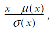
where μ(x) is mean value of the column and σ(x) is the standard deviation of the column. To normalize data, you can call the function scale_to_z_score() in the tensorflow_transform library. You can read the sidebar on tensorflow_transform to understand more about what the library offers. Then the function stores each feature in the outputs under a new key (via the _transformed_name function) derived from the original feature name (the new key is generated by appending _xf to the end of the original feature name).

Next, it treats the vocabulary-based categorical features (where names are stored in _VOCAB_FEATURE_KEYS) by converting each string to an index using a dictionary. The dictionary maps each string to an index and is learned from the provided training data automatically. This is similar to how we used the Keras Tokenizer object to learn a dictionary that we used to convert words to word IDs. In the tensorflow_transform library you have the handy compute_and_apply_vocabulary() function. To the compute_and_apply_vocabulary()function, we can pass num_oov_buckets=1 in order to assign any unseen strings to a special category (apart from the ones already assigned to known categories).

Afterward, the function tackles the to-be-bucketized features. Bucketization is the process of applying a continuous value to a bucket, where a bucket is defined by a set of boundaries. Bucketizing features can be achieved effortlessly with the apply_buckets() function, which takes the feature (provided in the inputs dictionary) and bucket boundaries as the input arguments.

Finally, we keep the column containing the label as it is. With that, we define the Transform component (http://mng.bz/mOGr).

from tfx.components import Transform
 
transform = Transform(
    examples=example_gen.outputs['examples'],
    schema=schema_gen.outputs['schema'],
    module_file=os.path.abspath('forest_fires_transform.py'),
)
 
context.run(transform)

The Transform component takes three inputs:

• Output examples of the CsvExampleGen component

• Schema from the SchemaGen

• The Python module that defines the preprocessing_fn() function for transforming data to features

One thing we must do when it comes to multi-component pipelines, like a TFX pipeline, is check every interim output whenever we can. It’s a much better choice than leaving things to chance and praying things work out fine (which is normally never the case). So, let’s inspect the output by printing some of the data saved to the disk after running the Transform step (see the next listing). The code for printing the data will be similar to when we printed the data when using the CsvExampleGen component.

Listing 15.5 Inspecting the outputs produced by the TFX Transform step

import forest_fires_constants
 
_DENSE_FLOAT_FEATURE_KEYS = forest_fires_constants.DENSE_FLOAT_FEATURE_KEYS
_VOCAB_FEATURE_KEYS = forest_fires_constants.VOCAB_FEATURE_KEYS
_BUCKET_FEATURE_KEYS = forest_fires_constants.BUCKET_FEATURE_KEYS
_LABEL_KEY = forest_fires_constants.LABEL_KEY
 
# Get the URI of the output artifact representing the training examples, which is a directory
train_uri = os.path.join(
    transform.outputs['transformed_examples'].get()[0].uri, 'Split-train'
)
tfrecord_filenames = [
    os.path.join(train_uri, name) for name in os.listdir(train_uri)        ❶
]
 
dataset = tf.data.TFRecordDataset(
    tfrecord_filenames, compression_type="GZIP"
)                                                                          ❷
 
 
example_records = []                                                       ❸
float_features = [
    _transformed_name(f) for f in _DENSE_FLOAT_FEATURE_KEYS + [_LABEL_KEY] ❹
]
int_features = [
    _transformed_name(f) for f in _BUCKET_FEATURE_KEYS + 
➥ _VOCAB_FEATURE_KEYS                                                     ❹
]
for tfrecord in dataset.take(5):                                           ❺
  serialized_example = tfrecord.numpy()                                    ❻
  example = tf.train.Example()                                             ❻
  example.ParseFromString(serialized_example)                              ❻
  record = [
    example.features.feature[f].int64_list.value for f in int_features     ❼
  ] + [
    example.features.feature[f].float_list.value for f in float_features   ❼
  ]
  example_records.append(record)                                           ❽
  print(example)
  print("="*50)

❶ Get the list of files in this directory (all compressed TFRecord files).

❷ Create a TFRecordDataset to read these files.

❸ Used to store the retrieved feature values (for later inspection)

❹ Dense (i.e., float) and integer (i.e., vocab-based and bucketized) features

❺ Get the first five examples in the data set.

❻ Get a tf record and convert that to a readable tf.train.Example.

❼ We will extract the values of the features from the tf.train.Example object for subsequent inspections.

❽ Append the extracted values as a record (i.e., tuple of values) to example_records.

The code explained will print the data after feature transformation. Each example stores integer values in the attribute path, example.features.feature[<feature name>] .int64_list.value, whereas the floating values are stored at example.features.feature [<feature name>].float_list.value. This will print examples such as

features {
  feature {
    key: "DC_xf"
    value {
      float_list {
        value: 0.4196213185787201
      }
    }
  }
 
  ...
 
  feature {
    key: "RH_xf"
    value {
      int64_list {
        value: 0
      }
    }
  }
 
  ...
 
  feature {
    key: "area_xf"
    value {
      float_list {
        value: 2.7699999809265137
      }
    }
  }
 
  ...
}

Note that we are using the _transformed_name() function to obtain the transformed feature names. We can see that the floating-point values (DC_xf) are normalized using z-score normalization, vocabulary-based features (day_xf) are converted to an integer, and bucketized features (RH_xf) are presented as integers.

In the next section, we will train a simple regression model as a part of the pipeline we’ve been creating.

Exercise 1

Let’s say that, instead of the previously defined feature transformations, you want to do the following:

• DC—Scale data to a range of [0, 1]

• temp—Bucketize with the boundaries (-inf, 20], (20, 30] and (30, inf)

Once the features are transformed, add them to a dictionary named outputs, where each feature is keyed by the transformed feature name. Assume you can obtain the transformed feature name for temp by calling, _transformed_name(‘temp’). How would you use the tensorflow_transform library to achieve this? You can use the scale_to_0_1() and apply_buckets() functions to achieve this.

15.2 Training a simple regression neural network: TFX Trainer API

You have defined a TFX data pipeline that can convert examples in a CSV file to model-ready features. Now you will train a model on this data. You will use TFX to define a model trainer, which will take a simple two-layer fully connected regression model and train that on the data flowing from the data pipeline. Finally, you will predict using the model on some sample evaluation data.

With a well-defined data pipeline defined using TFX, we’re at the cusp of training a model with the data flowing from that pipeline. Training a model with TFX can be slightly demanding at first sight due to the rigid structure of functions and data it expects. However, once you are familiar with the format you need to adhere to, it gets easier.

We will go through this section in three stages. First, let’s examine how we can define a Keras model to suit the output features we have defined in the TFX Transform component. Ultimately, the model will receive the output of the Transform component. Next, we will look at how we can write a function that encapsulates model training. This function will use the model defined and, along with several user-defined arguments, train the model and save it to a desired path. The saved model cannot be just any model; it has to have what are known as signatures in TensorFlow. These signatures dictate what the inputs to the model and outputs of the model look like when it’s finally used via an API. The API is served via a server that exposes a network port for the client to communicate with the API. Figure 15.6 depicts how the API ties in with the model.

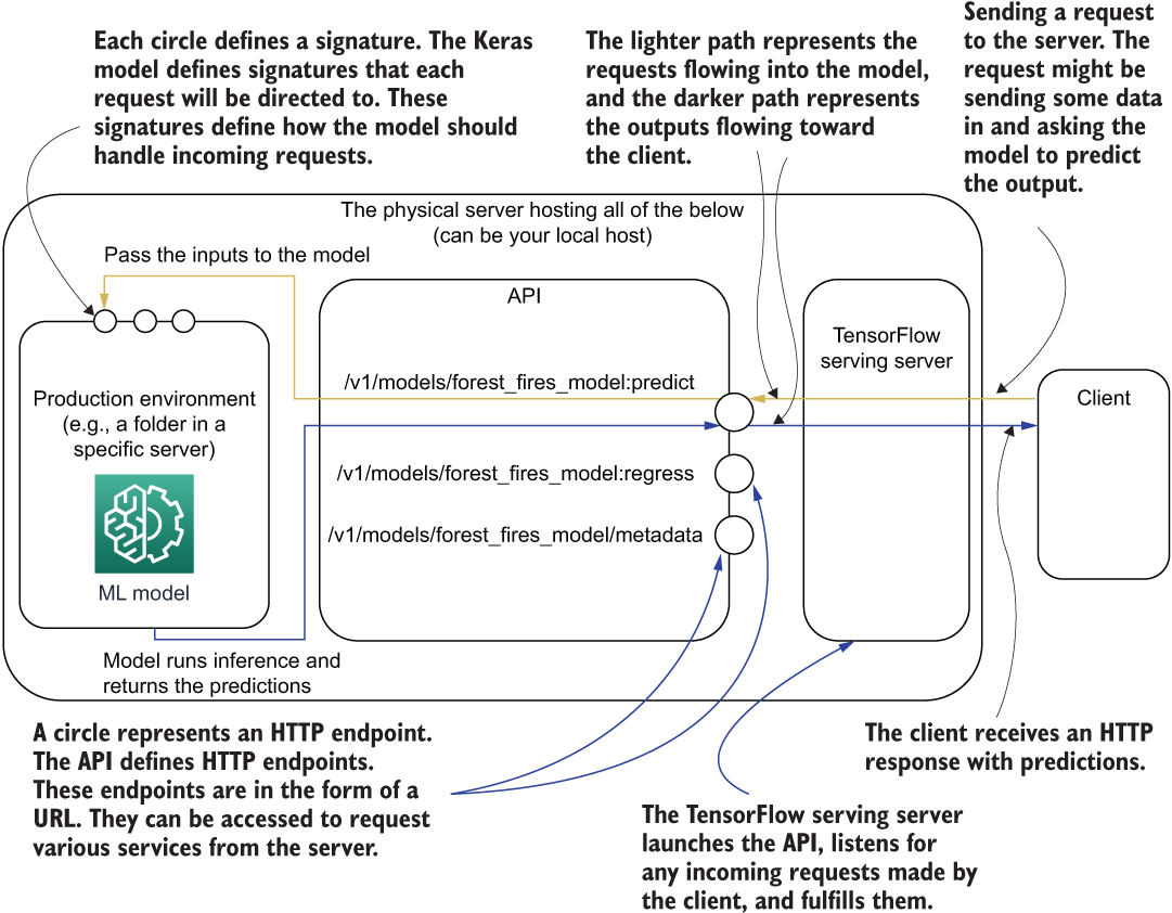
Figure 15.6 How the model interacts with the API, the TensorFlow server, and the client

Let’s understand what is taking place in figure 15.6. First, an HTTP client sends a request to the server. The server (i.e., a TensorFlow serving server) that is listening for any incoming requests will read the request and direct that to the required model signature. Once the data is received by the model signature, it will perform necessary processing on the data, run it through the model, and produce the output (e.g., predictions). Once the predictions are available, they will be returned by the server to the client. We will discuss the API and the server side in detail in a separate section. In this section, our focus is on the model.

We will circle back to signatures in a separate subsection to understand them in more detail. Finally, we will visually inspect model predictions by loading the model and feeding some data into it.

15.2.1 Defining a Keras model

The cornerstone for training the model with TFX is defining a model. There are two ways to define models for TFX: using the Estimator API or using the Keras API. We are going to go with the Keras API, as the Estimator API is not recommended for TensorFlow 2 (see the following sidebar for more details).

We are first going to create a function called _build_keras_model(), which will do two things. First, it will create tf.feature_column-type objects for all the features we have defined in our Transform step. tf.feature_column is a feature representation standard and is accepted by models defined in TensorFlow. It is a handy tool for defining data in a column-oriented fashion (i.e., each feature represented as a column). Columnar representation is very suitable for structured data, where each column typically is an independent predictor for the target variable. Let’s examine a few specific tf.feature_column types that are found in TensorFlow:

• tf.feature_column.numeric_column—Used to represent dense floating-point fields like temperature.

• tf.feature_column.categorical_column_with_identity—Used to represent categorical fields or bucketized fields where the value is an integer index pointing to a category or a bucket, such as day or month. Because the value passed to the column itself is the category ID, the term “identity” is used.

• tf.feature_column.indicator_column—Converts a tf.feature_column.categorical_column_with_identity to a one-hot encoded representation.

• tf.feature_column.embedding_column—Can be used to generate an embedding from an integer-based column like tf.feature_column.categorical_column_with_identity. It maintains an embedding layer internally and will return the corresponding embedding, given an integer ID.

To see the full list, refer to http://mng.bz/6Xeo. Here, we will use the top three types of tf.feature_columns as inputs to our to-be defined model. The following listing outlines how tf.feature_columns are used as inputs.

Listing 15.6 Building the Keras model using feature columns

def _build_keras_model() -> tf.keras.Model:                     ❶
  
  real_valued_columns = [                                       ❷
      tf.feature_column.numeric_column(key=key, shape=(1,))
      for key in _transformed_names(_DENSE_FLOAT_FEATURE_KEYS)
  ]
  
  categorical_columns = [                                       ❸
      tf.feature_column.indicator_column(
          tf.feature_column.categorical_column_with_identity(
              key, 
              num_buckets=len(boundaries)+1
          )
      ) for key, boundaries in zip(
          _transformed_names(_BUCKET_FEATURE_KEYS),
          _BUCKET_FEATURE_BOUNDARIES
      )
  ]
    
  categorical_columns += [                                      ❹
      tf.feature_column.indicator_column(
          tf.feature_column.categorical_column_with_identity( 
              key,
              num_buckets=num_buckets,
              default_value=num_buckets-1
          )
      ) for key, num_buckets in zip(
              _transformed_names(_VOCAB_FEATURE_KEYS),
              _MAX_CATEGORICAL_FEATURE_VALUES
      )      
  ]
 
  model = _dnn_regressor(                                       ❺
      columns=real_valued_columns+categorical_columns,          ❻
      dnn_hidden_units=[128, 64]                                ❼
  )
 
  return model

❶ Define the function signature. It returns a Keras model as the output.

❷ Create tf.feature_column objects for dense features.

❸ Create tf.feature_column objects for the bucketized features.

❹ Create tf.feature_column objects for the categorical features.

❺ Define a deep regressor model using the function.

❻ Uses the columns defined above

❼ It will have two intermediate layers: 128 nodes and 64 nodes.

Let’s look at the first set of feature columns stored in real_valued_columns. We take transformed names of the original keys of dense floating-point valued columns, and for each column, we create a tf.feature_column.numeric_column. You can see that we are passing

• A key (string)—Name of the feature

• A shape (a list/tuple)—Full shape will be derived as [batch size] + shape

For example, the column temp will have the key as temp_xf and shape as (1,), meaning that the full shape is [batch size, 1]. This shape of [batch size, 1] makes sense since each dense feature has a single value per record (meaning that we don’t need a feature dimensionality in the shape). Let’s go through a toy example to see a tf.feature_column.numeric_column in action:

a = tf.feature_column.numeric_column("a")
x = tf.keras.layers.DenseFeatures(a)({'a': [0.5, 0.6]})
print(x)

This will output

tf.Tensor(
[[0.5]
 [0.6]], shape=(2, 1), dtype=float32)

When defining tf.feature_column.categorical_column_with_identity for the bucketized features, you need to pass

• A key (string)—Name of the feature

• num_buckets (int)—Number of buckets in the bucketized feature

For instance, the RH feature that was bucketized will have the key RH_xf and num_buckets = 3, where the buckets are [[-inf, 33), [33, 66), [66, inf]]. Since we defined the bucket boundary for RH as (33, 66), num_buckets is defined as len(boundaries) +1 = 3. Finally, each categorical feature is wrapped in a tf.feature_column.indicator_column to convert each feature to one-hot encoded representation. Again, we can do a quick experiment to see the effects of these feature columns as follows:

b = tf.feature_column.indicator_column(
    tf.feature_column.categorical_column_with_identity('b', num_buckets=10)
)
y = tf.keras.layers.DenseFeatures(b)({'b': [5, 2]})
print(y)

This will produce

tf.Tensor(
[[0. 0. 0. 0. 0. 1. 0. 0. 0. 0.]
 [0. 0. 1. 0. 0. 0. 0. 0. 0. 0.]], shape=(2, 10), dtype=float32)

Finally, the vocabulary-based categorical features are treated similarly to the bucketized features. For each feature, we get the feature name and the maximum number of categories and define a tf.feature_column.categorical_column_with_identity column with

• key (string)—Name of the feature.

• num_buckets (int)—Number of categories.

• default_value (int)—If a previously unseen category is encountered, it will be assigned this value.

Here, default_value is an important part. It will dictate what happens to any unseen categories that might appear in the testing data and that weren’t a part of the training data. The vocabulary-based categorical features in our problem were day and month, which can only have 7 and 12 distinct values. But there could be situations where the training set only has 11 months and the test set has 12 months. To tackle this, we will assign any unseen category to the last category ID (i.e., num_buckets - 1) available to us.

We now have a collection of well-defined data columns that are wrapped in tf.feature_column objects ready to be fed to a model. Finally, we see a function called _dnn_regressor() that will create a Keras model, which is shown in the next listing, and pass the columns we create and some other hyperparameters. Let’s now discuss the specifics of this function.

Listing 15.7 Defining the regression neural network

def _dnn_regressor(columns, dnn_hidden_units):                            ❶
 
 
  input_layers = {
      colname: tf.keras.layers.Input(
          name=colname, shape=(), dtype=tf.float32
      )                                                                   ❷
      for colname in _transformed_names(_DENSE_FLOAT_FEATURE_KEYS)
  }
  input_layers.update({
      colname: tf.keras.layers.Input(
          name=colname, shape=(), dtype='int32'
      )                                                                   ❸
      for colname in _transformed_names(_VOCAB_FEATURE_KEYS)
  })
  input_layers.update({
      colname: tf.keras.layers.Input(
          name=colname, shape=(), dtype='int32'
      )                                                                   ❹
      for colname in _transformed_names(_BUCKET_FEATURE_KEYS)
  })  
 
  output = tf.keras.layers.DenseFeatures(columns)(input_layers)           ❺
  for numnodes in dnn_hidden_units:
    output = tf.keras.layers.Dense(numnodes, activation='tanh')(output)   ❻
  
  output = tf.keras.layers.Dense(1)(output)                               ❼
 
  model = tf.keras.Model(input_layers, output)                            ❽
  model.compile(
      loss='mean_squared_error',                                          ❾
      optimizer=tf.keras.optimizers.Adam(lr=0.001)
  )
  model.summary(print_fn=absl.logging.info)                               ❿
 
  return model

❶ Define a function that takes a bunch of columns and a list of hidden dimensions as the input.

❷ Inputs to the model: an input dictionary where the key is the feature name and the value is a Keras Input layer

❸ Update the dictionary by creating Input layers for vocabulary-based categorical features.

❹ Update the dictionary by creating Input layers for bucketized features.

❺ As input layers are defined as a dictionary, we use the DenseFeatures layer to generate a single tensor output.

❻ We recursively compute the output by creating a sequence of Dense layers.

❼ Create a final regression layer that has one output node and a linear activation.

❽ Define the model using inputs and outputs.

❾ Compile the model. Note how it uses the mean squared error as the loss function.

❿ Print a summary of the model through the absl logger we defined at the beginning.

We have defined the data in a columnar fashion, where each column is a TensorFlow feature column. Once the data defined in this way, we use a special layer called tf.keras.layers.DenseFeatures to process this data. The DenseFeatures layer accepts

• A list of feature columns

• A dictionary of tf.keras.layers.Input layers, where each Input layer is keyed with a column name found in the list of feature columns

With this data, the DenseFeatures layer can map each Input layer to the corresponding feature column and produce a single tensor output at the end (stored in the variable output) (figure 15.7).

Figure 15.7 Overview of the functionality of the DenseFeatures layer

Then we recursively compute the output by flowing the data through several hidden layers. The sizes of these hidden layers (a list of integers) are passed in as an argument to the function. We will use tanh nonlinear activation for the hidden layers. The final hidden output goes to a single node regression layer that has a linear activation.

Finally, we compile the model with the Adam optimizer and mean-squared loss as the loss function. It is important to note that we have to use a regression-compatible loss function for the model. The mean-squared error is a very common loss function chosen for regression problems.

def _build_keras_model() -> tf.keras.Model:

def run_fn(fn_args: tfx.components.FnArgs):

In listing 15.8, we define a function that, given a set of training data filenames and evaluation data filenames, generates tf.data.Dataset objects for training and evaluation data. We define this special function as _input_fn(). _input_fn() takes in three things:

• file_pattern—A set of file paths, where files contain data

• data_accessor—A special object in TFX that creates a tf.data.Dataset by taking in a list of filenames and other configuration

• batch_size—An integer specifying the size of a batch of data

Listing 15.8 A function to generate a tf.data.Dataset using the input files

from typing import List, Text                                ❶
 
def _input_fn(file_pattern: List[Text],                      ❷
              data_accessor: tfx.components.DataAccessor,    ❸
              tf_transform_output: tft.TFTransformOutput,    ❹
              batch_size: int = 200) -> tf.data.Dataset:     ❺
 
  return data_accessor.tf_dataset_factory(
      file_pattern,
      tfxio.TensorFlowDatasetOptions(
          batch_size=batch_size, label_key=_transformed_name(_LABEL_KEY)),
      tf_transform_output.transformed_metadata.schema)

❶ The typing library defines the type of inputs to the function.

❷ List of paths or patterns of input tfrecord files. It is a list of objects of type Text (i.e., strings).

❸ DataAccessor for converting input to RecordBatch

❹ A TFTransformOutput

❺ Represents the number of consecutive elements of the returned data set to combine in a single batch

You can see how we are using type hints for the arguments as well as the return object. The function returns a tf.data.Dataset obtained by calling the tf_dataset_factory() function with a list of file paths and data set options like batch size and label key. The label key is important for the data_accessor to determine input fields and the target. You can see that the data accessor takes in the schema from the Transform step as well. This helps the data_accessor to transform the raw examples to features and then separate the inputs and the label. With all the key functions explained, we now move on to see how all of these will be orchestrated in order to do the model training.

15.2.2 Defining the model training

The main task that’s standing between us and a train model is the actual training of the model. The TFX component responsible for training the model (known as Trainer) expects a special function named run_fn() that will tell how the model should be trained and eventually saved (listing 15.9). This function takes in a special type of object called FnArgs, a utility object in TensorFlow that can be used to declare model training-related user-defined arguments that need to be passed to a model training function.

Listing 15.9 Running the Keras model training with the data

def run_fn(fn_args: tfx.components.FnArgs):                        ❶
 
  absl.logging.info("="*50)
  absl.logging.info("Printing the tfx.components.FnArgs object")   ❷
  absl.logging.info(fn_args)                                       ❷
  absl.logging.info("="*50)
 
  tf_transform_output = tft.TFTransformOutput(
    fn_args.transform_graph_path
  )                                                                ❸
 
  train_dataset = _input_fn(
    fn_args.train_files, fn_args.data_accessor, tf_transform_output, 
➥ 40                                                              ❹
  )
  eval_dataset = _input_fn(
    fn_args.eval_files, fn_args.data_accessor, tf_transform_output, 
➥ 40                                                              ❹
  )
  model = _build_keras_model()                                     ❺
  
  csv_write_dir = os.path.join(
    fn_args.model_run_dir,'model_performance'
)                                                                  ❻
  os.makedirs(csv_write_dir, exist_ok=True)
 
  csv_callback = tf.keras.callbacks.CSVLogger(
    os.path.join(csv_write_dir, 'performance.csv'), append=False   ❼
  )
 
  model.fit(                                                       ❽
      train_dataset,
      steps_per_epoch=fn_args.train_steps,
      validation_data=eval_dataset,
      validation_steps=fn_args.eval_steps,
      epochs=10,
      callbacks=[csv_callback]
  )
 
  signatures = {                                                   ❾
      'serving_default':
          _get_serve_tf_examples_fn(
              model, tf_transform_output
          ).get_concrete_function(
              tf.TensorSpec(
                  shape=[None],
                  dtype=tf.string,
                  name='examples'
              )
          ),
      
  }
  model.save(fn_args.serving_model_dir, save_format='tf', signatures=signatures)                                        ❿

❶ Define a function called run_fn that takes a tfx.components.FnArgs object as the input.

❷ Log the values in the fn_args object.

❸ Load the tensorflow_transform graph.

❹ Convert the data in the CSV files to tf.data.Dataset objects using the function _input_fn (discussed soon).

❺ Build the Keras model using the previously defined function.

❻ Define a directory to store CSV logs produced by the Keras callback CSVLogger.

❼ Define the CSVLogger callback.

❽ Fit the model using the data sets created and the hyperparameters present in the fn_args object.

❾ Define signatures for the model. Signatures tell the model what to do when data is sent via an API call when the model is deployed.

❿ Save the model to the disk.

Let’s first check the method signature of the run_fn(). run_fn() takes in a single argument of type FnArgs as the input. As mentioned earlier, FnArgs is a utility object that stores a collection of key-value pairs that are useful for model training. Most of the elements in this object are populated by the TFX component itself. However, you also have the flexibility to pass some of the values. We will define some of the most important attributes in this object. But we will learn more about the full list of attributes once we see the full output produced by the TFX Trainer component. Table 15.2 provides you a taste of what is stored in this object. Don’t worry if you don’t fully understand the purpose of these elements. It will be clearer as we go through the chapter. Once we run the Trainer component, it will display the values used for every one of these attributes, as we have included logging statements to log the fn_args object. This will help us to contextualize these properties with the example we’re running and understand them more clearly.

Table 15.2 An overview of the attributes stored in the fn_args-type object

The first important task done by this function is generating tf.data.Dataset objects for training and evaluation data. We have defined a special function called _input_fn() that achieves this (listing 15.8).

Once the data sets are defined, we define the Keras model using the _build_keras_model() function we discussed earlier. Then we define a CSVLogger callback to log the performance metrics over epochs, as we did earlier. As a brief review, the tf.keras.callbacks.CSVLogger creates a CSV file with all the losses and metrics defined during model compilation, logged every epoch. We will use the fn_arg object’s model_run_dir attribute to create a path for the CSV file inside the model creation directory. This will make sure that if we run multiple training trials, each will have its own CSV file saved along with the model. After that, we call the model.fit() function as we have done countless times. The arguments we have used are straightforward, so we will not discuss them in detail and lengthen this discussion unnecessarily.

15.2.3 SignatureDefs: Defining how models are used outside TensorFlow

Once the model is trained, we have to store the model on disk so that it can be reused later. The objective of storing this model is to use this via a web-based API (i.e., a REST API) to query the model using inputs and get predictions out. This is typically how machine learning models are used to serve customers in an online environment. For models to understand web-based requests, we need to define things called SignatureDefs. A signature defines things like what an input or target to the model looks like (e.g., data type). You can see that we have defined a dictionary called signatures and passed it as an argument to model.save()(listing 15.9).

The signatures dictionary should have key-value pairs, where key is a signature name and value is a function decorated with the @tf.function decorator. If you want a quick refresher on what this decorator does, read the following sidebar.

It is also important to note that you cannot use arbitrary names as signature names. TensorFlow has a set of defined signature names, depending on your needs. These are defined in a special constant module in TensorFlow (http://mng.bz/o2Kd). There are four signatures to choose from:

• PREDICT_METHOD_NAME (value: 'tensorflow/serving/predict')—This signature is used to predict the target for incoming inputs. This does not expect the target to be present.

• REGRESS_METHOD_NAME (value: 'tensorflow/serving/regress')—This signature can be used to regress from an example. It expects both an input and an output (i.e., target value) to be present in the HTTP request body.

• CLASSIFY_METHOD_NAME (value: 'tensorflow/serving/classify')—This is similar to REGRESS_METHOD_NAME, except for classification. This signature can be used to classify an example. It expects both an input and an output (i.e., target value) to be present in the HTTP.

• DEFAULT_SERVING_SIGNATURE_DEF_KEY (value: 'serving_default')—This is the default signature name. A model should at least have the default serving signature in order to be used via an API. If none of the other signatures are defined, requests will go through this signature.

We will only define the default signature here. Signatures take a TensorFlow function (i.e., a function decorated with @tf.function) as a value. Therefore, we need to define a function (which we will call _get_serve_tf_examples_fn() ) that will tell TensorFlow what to do with an input (see the next listing).

Listing 15.10 Parsing examples sent through API requests and predicting from them

def _get_serve_tf_examples_fn(model, tf_transform_output):            ❶
 
  model.tft_layer = tf_transform_output.transform_features_layer()    ❷
 
  @tf.function
  def serve_tf_examples_fn(serialized_tf_examples):                   ❸
    """Returns the output to be used in the serving signature."""
    feature_spec = tf_transform_output.raw_feature_spec()             ❹
    feature_spec.pop(_LABEL_KEY)                                      ❺
    parsed_features = tf.io.parse_example(serialized_tf_examples, 
➥ feature_spec)                                                      ❻
    transformed_features = model.tft_layer(parsed_features)           ❼
    return model(transformed_features)                                ❽
 
  return serve_tf_examples_fn                                         ❾

❶ Returns a function that parses a serialized tf.Example and applies feature transformations

❷ Get the feature transformations to be performed as a Keras layer.

❸ The function decorated with @tf.function to be returned

❹ Get the raw column specifications.

❺ Remove the feature spec for the label as we do not want that during predictions.

❻ Parse the serialized example using the feature specifications.

❼ Convert raw columns to features using the layer defined.

❽ Return the output of the model after feeding the transformed features.

❾ Return the TensorFlow function.

The first important thing to note is that _get_serve_tf_examples_fn() returns a function (i.e., serve_tf_examples_fn), which is a TensorFlow function. The _get_serve_tf_examples_fn() accepts two inputs:

• Model—The Keras model we built during training time

• tf_transform_output—The transformation graph to convert raw data to features

This returned function should instruct TensorFlow on what to do with the data that came in through an API request once the model is deployed. The returned function takes serialized examples as inputs, parses them to be in the correct format as per the model input specifications, generates the output, and returns it. We will not dive too deeply into what the inputs and outputs are of this function, as we will not call it directly, but rather access TFX, which will access it when an API call is made.

In this process, the function first gets a raw feature specifications map, which is a dictionary of column names mapped to a Feature type. The Feature type describes the type of data that goes in a feature. For instance, for our data, the feature spec will look like this:

{
  'DC': VarLenFeature(dtype=tf.float32), 
  'DMC': VarLenFeature(dtype=tf.float32),
  'RH': VarLenFeature(dtype=tf.int64), 
  ...
  'X': VarLenFeature(dtype=tf.int64), 
  'area': VarLenFeature(dtype=tf.float32), 
  'day': VarLenFeature(dtype=tf.string), 
  'month': VarLenFeature(dtype=tf.string)
}

It can be observed that different data types are used (e.g., float, int, string) depending on the data found in that column. You can see a list of feature types at https://www.tensorflow.org/api_docs/python/tf/io/. Next, we remove the feature having the _LABEL_KEY as it should not be a part of the input. We then use the tf.io.parse_example() function to parse the serialized examples by passing the feature specification map. The results are passed to a TransformFeaturesLayer (http://mng.bz/nNRa) that knows how to convert a set of parsed examples to a batch of inputs, where each input has multiple features. Finally, the transformed features are passed to the model, which returns the final output (i.e., predicted forest burnt area). Let’s revisit the signature definition from listing 15.9:

signatures = {
      'serving_default':
          _get_serve_tf_examples_fn(
              model, tf_transform_output
          ).get_concrete_function(
              tf.TensorSpec(
                  shape=[None],
                  dtype=tf.string,
                  name='examples'
              )
          ),    
  }

You can see that we are not simply passing the returning TensorFlow function of _get_serve_tf_examples_fn(). Instead, we call the get_concrete_function() on the return function (i.e., TensorFlow function). If you remember from our previous discussions, when you execute a function decorated with @tf.function, it does two things:

• Traces the function and creates the data-flow graph to perform the work of the function

• Executes the graph to return outputs

get_concrete_function() does the first task only. In other words, it returns the traced function. You can read more about this at http://mng.bz/v6K7.

15.2.4 Training the Keras model with TFX Trainer

We now have all the bells and whistles to train the model. To reiterate, we first defined a Keras model, defined a function to run the model training, and finally defined signatures that instruct the model how to behave when an HTTP request is sent via the API. Now we will train the model as a part of the TFX pipeline. To train the model, we are going to use the TFX Trainer component:

from tfx.components import Trainer
from tfx.proto import trainer_pb2
import tensorflow.keras.backend as K
 
K.clear_session()
 
n_dataset_size = df.shape[0]
batch_size = 40
 
n_train_steps_mod = 2*n_dataset_size % (3*batch_size)
n_train_steps = int(2*n_dataset_size/(3*batch_size))
if n_train_steps_mod != 0:
    n_train_steps += 1
 
n_eval_steps_mod = n_dataset_size % (3*batch_size)
n_eval_steps = int(n_dataset_size/(3*batch_size))
if n_eval_steps != 0:
    n_eval_steps += 1
 
trainer = Trainer(
    module_file=os.path.abspath("forest_fires_trainer.py"),
    transformed_examples=transform.outputs['transformed_examples'],
    schema=schema_gen.outputs['schema'],
    transform_graph=transform.outputs['transform_graph'],
    train_args=trainer_pb2.TrainArgs(num_steps=n_train_steps),
    eval_args=trainer_pb2.EvalArgs(num_steps=n_eval_steps))
 
context.run(trainer)

The code leading up to the Trainer component simply computes the correct number of iterations required in an epoch. To calculate that, we first get the total size of the data (remember that we stored our data set in the DataFrame df). We then used two hash buckets for training and one for evaluation. Therefore, we would have roughly two-thirds training data and one-third evaluation data. Finally, if the value is not fully divisible, we add +1 to incorporate the remainder of the data.

Let’s investigate the instantiation of the Trainer component in more detail. There are several important arguments to pass to the constructor:

• module_file—Path to the Python module containing the run_fn().

• transformed_examples—Output of the TFX Transform step, particularly the transformed examples.

• schema—Output of the TFX SchemaGen step.

• train_args—A TrainArgs object specifying training-related arguments. (To see the proto message defined for this object, see http://mng.bz/44aw.)

• eval_args—An EvalArgs object specifying evaluation-related arguments. (To see the proto message defined for this object, see http://mng.bz/44aw.)

This will output the following log. Due to the length of the log output, we have truncated certain parts of the log messages:

INFO:absl:Generating ephemeral wheel package for 
➥ '/home/thushv89/code/manning_tf2_in_action/Ch15-TFX-for-MLOps-in-
➥ TF2/tfx/forest_fires_trainer.py' (including modules: 
➥ ['forest_fires_constants', 'forest_fires_transform', 
➥ 'forest_fires_trainer']).
 
...
 
INFO:absl:Training model.
 
...
 
43840.0703WARNING:tensorflow:11 out of the last 11 calls to <function 
➥ recreate_function.<locals>.restored_function_body at 0x7f53c000ea60> 
➥ triggered tf.function retracing. Tracing is expensive and the excessive 
➥ number of tracings could be due to (1) creating @tf.function repeatedly 
➥ in a loop, (2) passing tensors with different shapes, (3) passing 
➥ Python objects instead of tensors. 
 
INFO:absl:____________________________________________________________________________
INFO:absl:Layer (type)                    Output Shape         Param #    
➥ Connected to                     
INFO:absl:=================================================================
➥ ===========
 
...
 
INFO:absl:dense_features (DenseFeatures)  (None, 31)           0           
➥ DC_xf[0][0]                      
INFO:absl:                                                                
➥ DMC_xf[0][0]                     
INFO:absl:                                                               
➥ FFMC_xf[0][0]                    
...
INFO:absl:                                                               
➥ temp_xf[0][0]                    
INFO:absl:                                                               
➥ wind_xf[0][0]                    
INFO:absl:_________________________________________________________________
➥ ___________
 
...
 
INFO:absl:Total params: 12,417
 
...
 
Epoch 1/10
9/9 [==============================] - ETA: 3s - loss: 43840.070 - 1s 
➥ 32ms/step - loss: 13635.6658 - val_loss: 574.2498
Epoch 2/10
9/9 [==============================] - ETA: 0s - loss: 240.241 - 0s 
➥ 10ms/step - loss: 3909.4543 - val_loss: 495.7877
...
Epoch 9/10
9/9 [==============================] - ETA: 0s - loss: 42774.250 - 0s 
➥ 8ms/step - loss: 15405.1482 - val_loss: 481.4183
Epoch 10/10
9/9 [==============================] - 1s 104ms/step - loss: 1104.7073 - 
➥ val_loss: 456.1211
...
 
INFO:tensorflow:Assets written to: 
➥ /home/thushv89/code/manning_tf2_in_action/Ch15-TFX-for-MLOps-in-
➥ TF2/tfx/pipeline/examples/forest_fires_pipeline/Trainer/model/5/Format-
➥ Serving/assets
INFO:absl:Training complete. Model written to 
➥ /home/thushv89/code/manning_tf2_in_action/Ch15-TFX-for-MLOps-in-
➥ TF2/tfx/pipeline/examples/forest_fires_pipeline/Trainer/model/5/Format-
➥ Serving. ModelRun written to 
➥ /home/thushv89/code/manning_tf2_in_action/Ch15-TFX-for-MLOps-in-
➥ TF2/tfx/pipeline/examples/forest_fires_pipeline/Trainer/model_run/5
INFO:absl:Running publisher for Trainer
INFO:absl:MetadataStore with DB connection initialized

In the log message, we can see that the Trainer does a lot of heavy lifting. First, it creates a wheel package using the model training code defined in the forest_fires_trainer.py. wheel (extension .whl) is how Python would package a library. For instance, when you do pip install tensorflow, it will first download the wheel package with the latest version and install it locally. If you have a locally downloaded wheel package, you can use pip install <path to wheel>. You can find the resulting wheel package at the <path to pipeline root>/examples/forest_fires_pipeline/_wheels directory. Then it prints the model summary. It has an Input layer for every feature passed to the model. You can see that the DenseFeatures layer aggregates all these Input layers to produce a [None, 31]-sized tensor. As the final output, the model produces a [None, 1]-sized tensor. Then the model training takes place. You will see warnings such as

out of the last x calls to <function 
➥ recreate_function.<locals>.restored_function_body at 0x7f53c000ea60> 
➥ triggered tf.function retracing. Tracing is expensive and the excessive 
➥ number of tracings could be due to

This warning comes up when TensorFlow function tracing happens too many times. It can be a sign of poorly written code (e.g., the model getting recreated many times within a loop) and is sometimes unavoidable. In our case, it’s the latter. The behavior of the Trainer module is causing this behavior, and there’s not much we can do about that. Finally, the component writes the model as well as some utilities to a folder in the pipeline root. Here’s what our pipeline root directory looks like so far (figure 15.8).

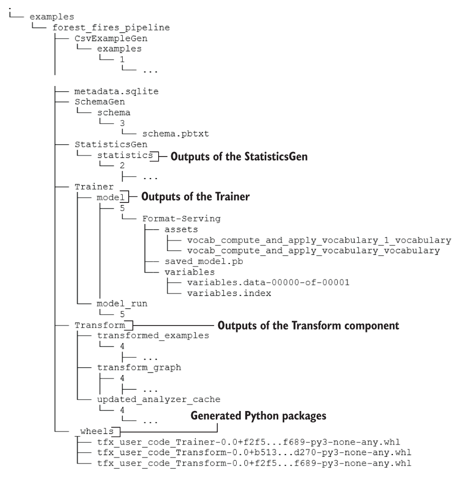
Figure 15.8 The complete directory/file structure after running the Trainer

A major issue we can note in the Trainer’s output log is the training and validation losses. For this problem, they are quite large. We are using the mean-squared error that is computed as

where N is the number of examples, y_i is the i^th example, and ŷ₁ is the predicted value for i^th example. At the end of the training, we have a squared loss of around 481, meaning an error of around 22 hectares (i.e., 0.22 km²) per example. This is not a small error. If you investigate this matter, you will realize this is largely caused by anomalies present in the data. Some anomalies are so large that they can skew the model heavily in the wrong direction. We will address this in an upcoming section in the chapter. You will be able to see the values in the FnArgs object passed to the run_fn():

INFO:absl:==================================================
INFO:absl:Printing the tfx.components.FnArgs object
INFO:absl:FnArgs(
    working_dir=None, 
    train_files=['.../Transform/transformed_examples/16/Split-train/*'], 
    eval_files=['.../Transform/transformed_examples/16/Split-eval/*'], 
    train_steps=100, 
    eval_steps=100, 
    schema_path='.../SchemaGen/schema/15/schema.pbtxt', 
    schema_file='.../SchemaGen/schema/15/schema.pbtxt', 
    transform_graph_path='.../Transform/transform_graph/16', 
    transform_output='.../Transform/transform_graph/16', 
    data_accessor=DataAccessor(
        tf_dataset_factory=<function 
➥ get_tf_dataset_factory_from_artifact.<locals>.dataset_factory at 
➥ 0x7f7a56329a60>, 
        record_batch_factory=<function 
➥ get_record_batch_factory_from_artifact.<locals>.record_batch_factory at 
➥ 0x7f7a563297b8>, 
        data_view_decode_fn=None
    ), 
    serving_model_dir='.../Trainer/model/17/Format-Serving', 
    eval_model_dir='.../Trainer/model/17/Format-TFMA', 
    model_run_dir='.../Trainer/model_run/17', 
    base_model=None, 
    hyperparameters=None, 
    custom_config=None
)
INFO:absl:==================================================

The following sidebar discusses how we can evaluate the model at this point in our discussion.

Next, we will discuss how we can detect anomalies present in the data and remove them to create a clean data set to train our model.

isi_feature = tfdv.get_feature(schema, 'ISI')
isi_feature.float_domain.max = 30.0

Next, we’ll look at a technology called Docker that is used for deploying models in isolated and portable environments. We will see how we can deploy our model in what is known as a Docker container.

Exercise 2

Instead of using one-hot encoding for day and month features and appending them to the categorical_columns variable, let’s imagine you want to use embeddings to represent these features. You can use the feature column tf.feature_column.embedding_column for this. Assume an embedding dimensionality of 32. You have the feature names of day and month columns stored in _VOCAB_FEATURE_KEYS (contains ['day', 'month']) and their dimensionality in _MAX_CATEGORICAL_FEATURE_VALUES (contains [7, 12]).

15.3 Setting up Docker to serve a trained model

You have developed a data pipeline and a robust model that can be used to predict the severity of forest fires based on the weather data. Now you want to go a step further and offer this as a more accessible service by deploying the model on a machine and enabling access through a REST API. This process is also known as productionizing a machine learning model. To do that, you are first going to create an isolated environment dedicated to model serving. The technology you will use is Docker.

CAUTION It is vitally important that you have Docker installed on your machine before proceeding further. To install Docker, follow the guide: https://docs.docker.com/engine/install/ubuntu/.

In TFX, you can deploy your model as a container, where the container is provisioned by Docker. According to the official Docker website, a Docker container is

a standard unit of software that packages up code and all its dependencies so the application runs quickly and reliably from one computing environment to another.

Source: https://www.docker.com/resources/what-container

Docker is a containerization technology that helps you run a software (or a microservice) isolated from the host. In Docker, you can create an image, which will instruct Docker with various specifications (e.g., OS, libraries, dependencies) that you need in the container for it to run the software correctly. Then a container is simply a run time instance of that image. This means you enjoy a higher portability as you can create a container on one computer and run it on another computer easily (as long as Docker is installed on two computers). Virtual machines (VMs) also try to achieve a similar goal. There are many resources out there comparing and contrasting Docker containers and VMs (e.g., http://mng.bz/yvNB).

As we have said, to run a Docker container, you first need a Docker image. Docker has a public image registry (known as Docker Hub) available at https://hub.docker.com/. The Docker image we are looking for is the TensorFlow serving image. This image has everything installed to serve a TensorFlow model, using the TensorFlow serving (https://github.com/tensorflow/serving), a sub-library in TensorFlow that can create a REST API around a given model so that you can send HTTP requests to use the model. You can download this image simply by running the following command:

docker pull tensorflow/serving:2.6.3-gpu

Let’s break down the anatomy of this command. docker pull is the command for downloading an image. tensorflow/serving is the image name. Docker images are version controlled, meaning every Docker image has a version tag (it defaults to the latest if you don’t provide one). 2.6.3-gpu is the image’s version. This image is quite large because it supports GPU execution. If you don’t have a GPU, you can use docker pull tensorflow/serving:2.6.3, which is more lightweight. Once the command successfully executes, you can run

docker images 

to list all the images you have downloaded. With the image downloaded, you can use the docker run <options> <Image> command to stand up a container using a given image. The command docker run is a very flexible command and comes with lots of parameters that you can set and change. We are using several of those:

docker run 
  --rm 
  -it 
  --gpus all 
  -p 8501:8501 
  --user $(id -u):$(id -g) 
  -v ${PWD}/tfx/forest-fires-pushed:/models/forest_fires_model 
  -e MODEL_NAME=forest_fires_model 
  tensorflow/serving:2.6.3-gpu

It’s important to understand the arguments provided here. Typically, when defining arguments in a shell environment, a single-dash prefix is used for single character-based arguments (e.g., -p) and a double-dash prefix is used for more verbose arguments (e.g., --gpus):

• --rm—Containers are temporary runtimes that can be removed after the service has run. --rm implies that the container will be removed after exiting it.

• -it (short for -i and -t)—This means that you can go into the container and interactively run commands in a shell within the container.

• --gpus all—This tells the container to ensure that GPU devices (if they exist) are visible inside the container.

• -p—This maps a network port in the container to the host. This is important if you want to expose some service (e.g., the API that will be up to serve the model) to the outside. For instance, TensorFlow serving runs on 8501 by default. Therefore, we are mapping the container’s 8501 port to the host’s 8501 port.

• --user $(id -u):$(id -g)—This means the commands will be run as the same user you’re logged in as on the host. Each user is identified by a user ID and is assigned to one or more groups (identified by the group ID). You can pass the user and the group following the syntax --user <user ID>:<group ID>. For example, your current user ID is given by the command id -u, and the group is given by id -g. By default, containers run commands as root user (i.e., running via sudo), which can make your services more vulnerable to outside attacks. So, we use a less-privileged user to execute commands in the container.

• -v—This mounts a directory on the host to a location inside the container. By default, things you store within a container are not visible to the outside. This is because the container has its own storage space/volume. If you need to make the container see something on the host or vice versa, you need to mount a directory on the host to a path inside the container. This is known as bind mounting. For instance, here we expose our pushed model (which will be at ./tfx/forest-fires-pushed) to the path /models/forest_fires_model inside the container.

• -e—This option can be used to pass special environment variables to the container. For example, the TensorFlow serving service expects a model name (which will be a part of the URL you need to hit in order to get results from the model).

This command is provided to you in the tfx/run_server.sh script in the Ch15-TFX-for-MLOps-in-TF2 directory. Let’s run the run_server.sh script to see what we will get. To run the script

1. Open a terminal.

2. Move cd into the Ch15-TFX-for-MLOps-in-TF2/tfx directory.

3. Run ./run_server.sh.

It will show an output similar to the following:

2.6.3-gpu: Pulling from tensorflow/serving
Digest: 
➥ sha256:e55c44c088f6b3896a8f66d8736f38b56a8c5687c105af65a58f2bfb0bf90812
Status: Image is up to date for tensorflow/serving:2.6.3-gpu
docker.io/tensorflow/serving:2.6.3-gpu
2021-07-16 05:59:37.786770: I
tensorflow_serving/model_servers/server.cc:88] Building single TensorFlow 
➥ model file config: model_name: forest_fires_model model_base_path: 
➥ /models/forest_fires_model
2021-07-16 05:59:37.786895: I
tensorflow_serving/model_servers/server_core.cc:464] Adding/updating 
➥ models.
2021-07-16 05:59:37.786915: I
tensorflow_serving/model_servers/server_core.cc:587]  (Re-)adding model: 
➥ forest_fires_model
2021-07-16 05:59:37.787498: W
tensorflow_serving/sources/storage_path/file_system_storage_path_source.cc:
➥ 267] No versions of servable forest_fires_model found under base path 
➥ /models/forest_fires_model. Did you forget to name your leaf directory 
➥ as a number (eg. '/1/')?
...

Of course, it will not work fully, as the directory we provided as model’s location is not populated. We still need to do a few things to have the final model in the right location.

In the next section, we will complete the rest of our pipeline. We will see how we can automatically evaluate as new models are trained in the pipeline, deploy the model if the performance is good, and enable prediction from the model using a REST API (i.e., a web-based API).

Exercise 3

Say you want to download the TensorFlow Docker image (it has the name tensorflow/ tensorflow) with version 2.5.0 and stand up a container that mounts the /tmp/inputs directory on your computer to /data volume within the container. Additionally, you would like to map the 5000 port in the container to 5000 on your computer. How would you do this using Docker commands? You can assume you’re running the commands as the root within the container.

15.4 Deploying the model and serving it through an API

You now have a data pipeline, a trained model, and a shell script that can run a Docker container with everything needed to run the model and the API to access the model. Now, using some services provided in TFX, you will deploy the model within a Docker container and make it available to be used through an API. In this process, you will run steps to validate the infrastructure (e.g., the container can be run and is healthy) and the model (i.e., when a new version of the model comes out, check if it is better than the last one), and finally, if everything is good, deploy the model on the infrastructure.

It has been a long journey. Let’s look back and see what we’ve accomplished so far. We have used the following TFX components:

• CsvExampleGen—Load data as TFRecord objects from CSV files.

• StatisticsGen—Basic statistics and visualizations about the distribution of various columns in the CSV data.

• SchemaGen—Generate the schema/template of the data (e.g., data types, domains, minimum/maximum values allowed, etc.).

• Transform—Transform the raw columns to features using the operations available in the tensorflow_transform library (e.g., one-hot encoding, bucketizing).

• Trainer—Define a Keras model, train it using the transformed data, and save to the disk. This model has a signature called serving default, which instructs the model what to do for an incoming request.

• ExampleValidator—This is used to validate that training and evaluation examples used adhere to the defined schema and can be used to detect anomalies.

15.4.1 Validating the infrastructure

Using TFX, you can ensure almost everything works well when you have a fully automated pipeline. We will discuss one such step here: the infrastructure validation step. In this, tfx.components.InfraValidator will automatically

• Create a container using a specific version of the TensorFlow serving image provided

• Load and run the model in it

• Send several requests to make sure the model responds

• Stand down the container

Let’s look at how we can use this component to validate the local Docker configuration we set up in the previous section (see the next listing).

Listing 15.11 Defining the InfraValidator

from tfx.components import InfraValidator
from tfx.proto import infra_validator_pb2
 
infra_validator = InfraValidator(
    model=trainer.outputs['model'],                                        ❶
    
    examples=example_gen.outputs['examples'],                              ❷
    serving_spec=infra_validator_pb2.ServingSpec(                          ❸
        tensorflow_serving=infra_validator_pb2.TensorFlowServing(          ❹
            tags=['2.6.3-gpu']
        ),
        local_docker=infra_validator_pb2.LocalDockerConfig(),              ❺
    ),
    request_spec=infra_validator_pb2.RequestSpec(                          ❻
        tensorflow_serving=infra_validator_pb2.TensorFlowServingRequestSpec(❼
            signature_names=['serving_default']
        ),
        num_examples=5                                                     ❽
    )
)
 
context.run(infra_validator)

❶ InfraValidator needs the location of the model it’s going to validate.

❷ Source for the data that will be used to build API calls to the model

❸ Holds a collection of model serving-related specifications

❹ Defines the version/tag of the TensorFlow serving Docker Image to be used

❺ Says to the InfraValidator that we are going to use the local Docker service to test

❻ Holds a collection of specifications related to the specific call made to the model

❼ Defines which model signature to use

❽ Defines how many requests to make to the model

The InfraValidator, just like any other TFX component, expects several arguments to run accurately:

• model—The Keras model returned by the Trainer component.

• examples—Loaded raw examples given by the CSVExampleGen.

• serving_spec—Expects a ServingSpec protobuf message. It will specify the version of the TensorFlow serving Docker image and whether to use local Docker installation (which is done here).

• request_spec—A RequestSpec protobuf message that will specify the signature that needs to be reached to verify the model is working.

If this step completes error-free, you will see the files shown in figure 15.9 in the pipeline root.

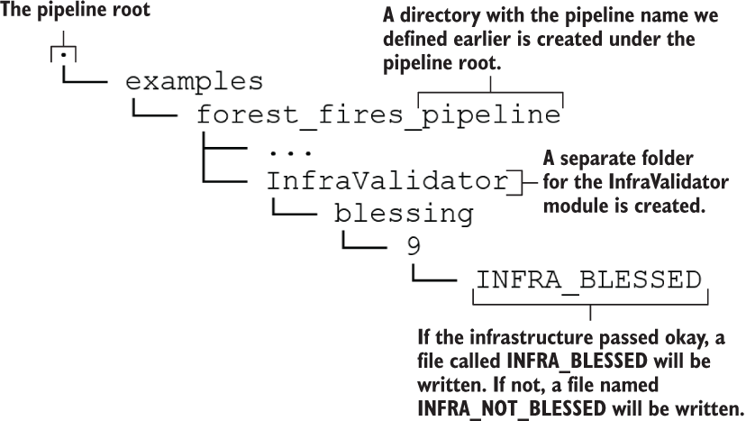
Figure 15.9 The directory/file structure after running the InfraValidator

You can see a file called INFRA_BLESSED appearing in the InfraValidator sub-directory. This brings us to the concept of blessing. TFX will bless certain elements in the pipeline when they run successfully. Once blessed, it will create a file with the suffix BLESSED. If the step fails, then a file with the suffix NOT_BLESSED will be created. Blessing helps to discriminate between things that ran fine and things that failed. For examples, once blessed, we can be sure that the infrastructure is working as expected. This means that things like

• Standing up a container

• Loading the model

• Reaching a defined API endpoint

can be performed without issues.

15.4.2 Resolving the correct model

Moving forward, we will define a resolver. The purpose of the resolver is to resolve a special artifact (like a model) that can evolve over time using a well-defined strategy (e.g., the model with the lowest validation error). Then the resolver informs subsequent components (e.g., the model Evaluator component we will be defining next) which artifact version to use. As you might have guessed, we will use the resolver to resolve the trained Keras model in the pipeline. So, if you run the pipeline multiple times, the resolver will make sure the latest and greatest model is used in the downstream components:

from tfx import v1 as tfx
 
model_resolver = tfx.dsl.Resolver(
      strategy_class=tfx.dsl.experimental.LatestBlessedModelStrategy,
      model=tfx.dsl.Channel(type=tfx.types.standard_artifacts.Model),
      model_blessing=tfx.dsl.Channel(
          type=tfx.types.standard_artifacts.ModelBlessing
      )
).with_id('latest_blessed_model_resolver')
 
context.run(model_resolver)

When defining the resolver to validate a model, we will define three things:

• strategy_class (a class from the tfx.dsl.components.common.resolver.ResolverStrategy namespace)—Defines the resolution strategy. There are two strategies supported currently: the latest blessed model (i.e., the model that has passed a set of defined evaluation checks) and the latest model.

• model (tfx.dsl.Channel)—Wraps a TFX artifact-type model in a tfx.dsl.Channel object. A tfx.dsl.Channel is an TFX-specific abstract concept that connects data consumers and data producers. For example, a channel is required to choose the correct model from a pool of models available in the pipeline.

• model_blessing (tfx.dsl.Channel)—Wraps a TFX artifact of type ModelBlessing in a tfx.dsl.Channel object.

You can look at various artifacts that you can wrap in a tfx.dsl.Channel object at http://mng.bz/2nQX.

15.4.3 Evaluating the model

We will evaluate the model as the last step before pushing it to a designated production environment. Essentially, we will define several evaluation checks that the model needs to pass. When a model is passed, TFX will bless the model. Otherwise, TFX will leave the model unblessed. We will learn later how to check if the model was blessed. To define the evaluation checks, we are going to use the tensorflow_model_analysis library. The first step is to define an evaluation configuration that specifies the checks:

import tensorflow_model_analysis as tfma
 
eval_config = tfma.EvalConfig(
    model_specs=[
        tfma.ModelSpec(label_key='area')                                  ❶
    ],
    metrics_specs=[
        tfma.MetricsSpec(
            metrics=[                                                     ❷
                tfma.MetricConfig(class_name='ExampleCount'),             ❸
                tfma.MetricConfig(
                    class_name='MeanSquaredError',                        ❹
                    threshold=tfma.MetricThreshold(                       ❺
                       value_threshold=tfma.GenericValueThreshold(
                           upper_bound={'value': 200.0}
                       ),
                       change_threshold=tfma.GenericChangeThreshold(      ❻
                           direction=tfma.MetricDirection.LOWER_IS_BETTER,
                           absolute={'value': 1e-10}
                       )
                   )
               )
           ]
        )
    ],
    slicing_specs=[                                                       ❼
        tfma.SlicingSpec(),                                               ❽
        tfma.SlicingSpec(feature_keys=['month'])                          ❾
    ])

❶ Define a model spec containing the label feature name.

❷ Define a list of metric specifications.

❸ Get the number of examples evaluated on.

❹ Define the mean-squared error as a metric.

❺ Define a threshold upper bound as a check.

❻ Define Change in error (compared to previous models) as a check (i.e., the lower the error the better).

❼ Slicing specs define how data needs to be partitioned when evaluating.

❽ Evaluate on the whole data set without slicing (i.e., an empty slice).

❾ Evaluate on partitioned data, where data is partitioned based on the month field.

The EvalConfig is quite a mouthful. Let’s go through it slowly. We have to define three things: model specifications (as a ModelSpec object), metric specifications (as a list of MetricsSpec objects), and slicing specifications (as a list of SlicingSpec objects). The ModelSpec object can be used to define the following:

• name—An alias model name that can be used to identify the model in this step.

• model_type—A string identifying the type of model. Allowed values include tf_keras, tf_estimator, tf_lite, and tf_js, tf_generic. For Keras models like ours, type is automatically derived.

• signature_name—The model signature to be used for inference. By default, serving_default is used.

• label_key—The name of the label feature in the examples.

• label_keys—For multi-output models, a list of label keys is used.

• example_weight_key—An optional key (or feature name) to retrieve example weights if present.

For more information about the ModelSpec object, refer to http://mng.bz/M5wW. In a MetricsSpec object, the following attributes can be set:

• metrics—A list of MetricConfig objects. Each MetricConfig object takes a class_name as an input. You can choose any class defined in tfma.metrics.Metric (http://mng.bz/aJ97) or tf.keras.metrics.Metric (http://mng.bz/gwmV) namespaces.

The SlicingSpec defines how the data needs to be partitioned during evaluation. For example, for time series problems, you will need to see how the model performs across different months or days. For that, SlicingSpec is a handy config. SlicingSpec has the following arguments:

• feature_keys—Can be used to define a feature key on which you can partition the data. For example, for feature key month, it will create a partition of data for each month by selecting data having a specific month. If not passed, it will return the whole data set.

Note that TFX uses the evaluation split you defined at the very beginning of the pipeline (i.e., when implementing the CsvExampleGen component) if not provided. In other words, all the metrics are evaluated on the evaluation split of the data set. Next, it defines two criteria for the evaluation to pass:

• The mean squared error is smaller than 200.

• The mean squared loss has improved by 1e - 10.

A model will be blessed (i.e., marked as passed) if these two conditions are satisfied for a newly trained model. Remember that we have seen a loss of around 150 in our better model, so let’s set the threshold to 200. The metrics added here are in addition to those saved when using the model.compile() step. For example, since the mean-squared error is used as the loss, it will already be a part of the metrics (even without defining it in eval_config).

Finally, we define the Evaluator (http://mng.bz/e7BQ) that will take in a model and run the evaluation checks defined in eval_config. You can define a TFX Evaluator as follows by passing in values for examples, model, baseline_model, and eval_ config arguments. baseline_model is resolved by the Resolver:

from tfx.components import Evaluator
 
evaluator = Evaluator(
    examples=example_gen.outputs['examples'],
    model=trainer.outputs['model'],
    baseline_model=model_resolver.outputs['model'],
    eval_config=eval_config)
context.run(evaluator)

Unfortunately, running the Evaluator will not provide the results you need. It will, in fact, fail the evaluation. At the bottom of the log, you will see an output like this

INFO:absl:Evaluation complete. Results written to 
➥ .../pipeline/examples/forest_fires_pipeline/Evaluator/evaluation/14.
INFO:absl:Checking validation results.
INFO:absl:Blessing result False written to 
➥ .../pipeline/examples/forest_fires_pipeline/Evaluator/blessing/14.

which says Blessing resulted False. It’s still a mystery why the model failed, given it showed only a loss of around 150 and we set the threshold to 200. To understand what happened, we need to look at the results written to the disk. If you look inside the <pipeline root>/ examplesforest_fires_pipelineEvaluator<execution ID> directory, you will see files like validation, metrics, and so forth. Along with the tensorflow_model_analysis library, these can provide invaluable insights to understand what when wrong. The tensorflow_model_analysis library provides several convenient functions to load the results stored in these files:

import tensorflow_model_analysis as tfma
 
validation_path = os.path.join(
    evaluator.outputs['evaluation']._artifacts[0].uri, "validations"
)
validation_res = tfma.load_validation_result(validation_path)
 
print('='*20, " Output stored in validations file ", '='*20)
print(validation_res)
print("="*75)

This will print out

metric_validations_per_slice {
  slice_key {
    single_slice_keys {
      column: "month"
      bytes_value: "sep"
    }
  }
  failures {
    metric_key {
      name: "mean_squared_error"
    }
    metric_threshold {
      value_threshold {
        upper_bound {
          value: 200.0
        }
      }
    }
    metric_value {
      double_value {
        value: 269.11712646484375
      }
    }
  }
}
validation_details {
  slicing_details {
    slicing_spec {
    }
    num_matching_slices: 12
  }
}

You can clearly see what happened. It says that the slice created for the month "sep" resulted in an error of 269, which is why our evaluation failed. If you want details about all of the slices used and their results, you can inspect the metrics file:

metrics_path = os.path.join(
    evaluator.outputs['evaluation']._artifacts[0].uri, "metrics"
)
metrics_res = tfma.load_metrics(metrics_path)
 
print('='*20, " Output stored in metrics file ", '='*20)
for r in metrics_res:
    print(r)
    print('-'*75)
print("="*75)

This would output the following. You will only see a small snippet of the full output here to save space:

slice_key {
  single_slice_keys {
    column: "month"
    bytes_value: "sep"
  }
}
metric_keys_and_values {
  key {
    name: "loss"
  }
  value {
    double_value {
      value: 269.11712646484375
    }
  }
}
metric_keys_and_values {
  key {
    name: "mean_squared_error"
  }
  value {
    double_value {
      value: 269.11712646484375
    }
  }
}
metric_keys_and_values {
  key {
    name: "example_count"
  }
  value {
    double_value {
      value: 52.0
    }
  }
}
 
---------------------------------------------------------------------------
slice_key {
}
metric_keys_and_values {
  key {
    name: "loss"
  }
  value {
    double_value {
      value: 160.19691467285156
    }
  }
}
metric_keys_and_values {
  key {
    name: "mean_squared_error"
  }
  value {
    double_value {
      value: 160.19691467285156
    }
  }
}
metric_keys_and_values {
  key {
    name: "example_count"
  }
  value {
    double_value {
      value: 153.0
    }
  }
}
...

This output sheds more light on what happened. Since we used the example count as one of the metrics, we can see the number of examples in each slice. For example, in month May, there’s only one example present in the evaluation split, which is most probably an outlier. To fix this, we will bump up the threshold to 300. Once you do that, you need to rerun the Evaluator, and you will see from the Evaluator’s logs that our model passes the checks:

INFO:absl:Evaluation complete. Results written to 
➥ .../pipeline/examples/forest_fires_pipeline/Evaluator/evaluation/15.
INFO:absl:Checking validation results.
INFO:absl:Blessing result True written to 
➥ .../pipeline/examples/forest_fires_pipeline/Evaluator/blessing/15.

The best way to address this is to identify why the month of "sep" is giving such a large value while other months are on par with or below the overall loss value. After identifying the issue, we should identify remediation steps to correct this (e.g., reconsidering outlier definitions). On that note, we will move on to the next part of our pipeline.

15.4.4 Pushing the final model

We have reached the last steps in our pipeline. We need to define a Pusher. The Pusher (http://mng.bz/pOZz) is responsible for pushing a blessed model (i.e., a model that passes the evaluation checks) to a defined production environment. The production environment can simply be a local location in your file system:

from tfx.components import Pusher
from tfx.proto import pusher_pb2
 
pusher = Pusher(
  model=trainer.outputs['model'],
  model_blessing=evaluator.outputs['blessing'],
  infra_blessing=infra_validator.outputs['blessing'],
  push_destination=pusher_pb2.PushDestination(
    filesystem=pusher_pb2.PushDestination.Filesystem(
        base_directory=os.path.join('forestfires-model-pushed'))
  )
)
context.run(pusher)

The Pusher takes the following elements as arguments:

• model—The Keras model returned by the Trainer component

• model_blessing—Evaluator component’s blessed state

• infra_blessing—InfraValidator’s blessed state

• push_destination—A destination to be pushed to as a PushDestination protobuf message

If the step runs successfully, you will have a model saved in a directory called forestfires-model-pushed in our pipeline root.

15.4.5 Predicting with the TensorFlow serving API

The very last step is to retrieve the model from the pushed destination and start a Docker container based on the TensorFlow serving image we downloaded. The Docker container will provide an API that we can ping with various requests.

Let’s look at how the API fits into the big picture in more detail (figure 15.10). The machine learning model sits behind an API. The API defines various HTTP endpoints you can ping (through Python or a package like curl). These endpoints will be in the form of a URL and can expect parameters in the URL or data embedded in the request body. The API is served via a server. The server exposes a network port in which clients can communicate with the server. The client can send requests to the server using the format <host name>:<port>/<end point>. We will discuss what the request actually looks like in more detail.

Figure 15.10 How the model interacts with the API, the TensorFlow server, and the client

To start the container, simply

1. Open a terminal

2. Move the cd into the Ch15-TFX-for-MLOps-in-TF2/tfx directory

3. Run ./run_server.sh

Next, in the Jupyter notebook, we will send a HTTP POST request. There are two main types of HTTP requests: GET and POST. Refer the sidebar if you’re interested in the differences. An HTTP POST request is a request that not only contains a URL to reach and header information, but also contains a payload, which is necessary for the API to complete the request. For example, if we are hitting the API endpoint corresponding to the serving_default signature, we have to send an input to predict with.

We will define a request body, which contains the signature name we want to hit and the input we want to predict for. Next, we will use the requests library in Python to send a request to our TensorFlow model server (i.e., Docker container). In this request, we will define the URL to reach (automatically generated by the TensorFlow model server) and the payload to carry. If the request is successful, we should get a valid prediction as the output:

import base64
import json
import requests
 
req_body = {
  "signature_name": "serving_default",
 
  "instances": 
    [
            str(base64.b64encode(
                b"{"X": 7,"Y": 
➥ 4,"month":"oct","day":"fri","FFMC":60,"DMC":30,"DC":200,
➥ "ISI":9,"temp":30,"RH":50,"wind":10,"rain":0}]")
               )
    ]
    
}
 
data = json.dumps(req_body)
 
json_response = requests.post(
    'http:/ /localhost:8501/v1/models/forest_fires_model:predict', 
    data=data, 
    headers={"content-type": "application/json"}
)
predictions = json.loads(json_response.text)

The first thing we do is define a request with a specific request body. The requirements for the request body are defined at https://www.tensorflow.org/tfx/serving/api_rest. It is a dictionary of key-value pairs that should have two keys: signature_name and instances. signature_name defines which signature to invoke in the model, and instances will contain the input data. Note that we’re not passing input data in its raw form. Rather, we use base64 encoding. It encodes a byte stream (i.e., a binary input) to an ASCII text string. You can read more about this at http://mng.bz/1o4g. You can see that we are first converting our dictionary to a byte-stream (i.e., with a b"<data>" format) and then using base64 encoding on that. If you remember from our previous discussion on writing the model serve function (which had the signature def serve_tf_examples_fn(serialized_tf_examples): ), it expects a serialized set of examples. Serialization is done by converting the data to a byte stream.

When the data is ready, we use the requests library to create a POST request for the API. First, we define a header to say that the content or payload we’re passing is JSON. Next, we send a POST request via requests.post() giving the URL, which is in http://<server’s hostname>:<port>/v1/models/<model name>:predict format, data (i.e., the JSON payload), and the header. This is not the only API endpoint available to us. There are other endpoints as well (https://www.tensorflow.org/tfx/serving/api_rest). There are four main endpoints that are available:

• http:/ /<server’s hostname>:<port>/v1/models/<model name>:predict—Predicts the output value using the model and the data passed in the request. Does not require a target to be available for the provided input.

• http:/ /<server’s hostname>:<port>/v1/models/<model name>:regress —Used in regression problems. Used when both inputs and target are available (i.e., an error can be calculated).

• http:/ /<server’s hostname>:<port>/v1/models/<model name>:classify—Used in classification problems. Used when both inputs and target are available (i.e., an error can be calculated).

• http:/ /<server’s hostname>:<port>/v1/models/<model name>/metadata—Provides metadata about available endpoints/model signatures.

This will return some response. If the request was successful, it will have the response; otherwise, it will contain an HTTP error. You can see various HTTP status/error codes at http://mng.bz/Pn2P. In our case, we should get something like

{'predictions': [[2.77522683]]}

This means our model has successfully processed the input and produced a valid prediction. We can see that the model has returned a prediction that is well within the possible range of values we saw during our data exploration. This concludes our discussion of TensorFlow Extended (TFX).

Exercise 4

How would you send multiple inputs in your HTTP request to the model? Assume you have the following two inputs that you want to predict for using the model.

To pass multiple values for that input in an HTTP request, you can append more examples to the instances list in the JSON data.

Summary

• MLOps defines a workflow that will automate most of the steps, from collecting data to delivering a model trained on that data.

• Productionization involves deploying a trained model with a robust API to access the model, enabling customers to use the model for its designed purpose. The API provides several HTTP endpoints, which are in the form of URLs, which clients can use to communicate with the server.

• In TFX, you define a MLOps pipeline as a series of TFX components.

• TFX has components to load data (CsvExampleGen), generate basic statistics and visualizations (StatisticsGen), infer the schema (SchemaGen), and convert raw columns to features (Transform).

• For a Keras model to be served via HTTP requests, signatures are required.

  • Signatures define the data format of inputs and outputs as well as the steps that need to happen in order to produce the output via a TensorFlow function (e.g., a function decorated with @tf.function).

• Docker is a containerization technology that can be used to encapsulate a unit of software as a single container and can be ported easily between different environments (or computers).

• Docker runs a unit of software in a container.

• TFX provides validation components for validating infrastructure and the model. TFX can stand up a container and make sure it’s running as expected, as well as make sure the model passes various evaluation criteria (e.g., loss being smaller than a threshold), ensuring a high-quality model.

• Once the model is pushed to a production environment, we start a Docker container (based on the TensorFlow serving image) that will mount the model into the container and serve it via an API. We can make HTTP requests (with the inputs embedded) to generate predictions.

Answers to exercises

Exercise 1

  outputs = {}
    
  # Treating dense features
  outputs[_transformed_name('DC')] = tft.scale_to_0_1(
        sparse_to_dense(inputs['DC'])
    )
 
 
  # Treating bucketized features
  outputs[_transformed_name('temp')] = tft.apply_buckets(
        sparse_to_dense(inputs['temp']), bucket_boundaries=[(20, 30)])

Exercise 2

categorical_columns = [
      tf.feature_column.embedding_column(
          tf.feature_column.categorical_column_with_identity( 
              key,
              num_buckets=num_buckets,
              default_value=0
          ),
          dimension=32
      ) for key, num_buckets in zip(
              _transformed_names(_VOCAB_FEATURE_KEYS),
              _MAX_CATEGORICAL_FEATURE_VALUES
      )

Exercise 3

docker run -v /tmp/inputs:/data -p 5000:5000 tensorflow/tensorflow:2.5.0

Exercise 4

req_body = {
  "signature_name": "serving_default",
 
  "instances": 
    [
        str(base64.b64encode(
            b"{"X": 9,"Y": 
➥ 6,"month":"aug","day":"fri","FFMC":91,"DMC":248,"DC":553,
➥ "ISI":6,"temp":20.5,"RH":58,"wind":3,"rain":0}]")
        ),
        str(base64.b64encode(
            b"{"X": 7,"Y": 
➥ 4,"month":"aug","day":"fri","FFMC":91,"DMC":248,"DC":553,
➥ "ISI":6,"temp":20.5,"RH":20,"wind":0,"rain":0}]")
        ),
        
    ]
    
}