14 TensorBoard: Big brother of TensorFlow

This chapter covers

• Running and visualizing image data in TensorBoard
• Monitoring model performance and behaviors in real time
• Performance profiling models using TensorBoard
• Using tf.summary to log custom metrics during customized model training
• Visualizing and analyzing word vectors on TensorBoard

Thus far we have focused on various models. We have talked about fully connected models (e.g., autoencoders), convolutional neural networks, and recurrent neural networks (e.g., LSTMs, GRUs). In chapter 13, we talked about Transformers, a powerful family of deep learning models that have paved the way to a new state-of-the-art performance in language understanding. Furthermore, inspired by the achievements in the field of natural language processing, Transformers are making waves in the computer vision field. We are past the modeling step, but we still have to plough through several more steps to reap the final harvest. One such step is making sure the data/features to the model are correct and the models are working as expected.

In this chapter, we will explore a new facet of machine learning: leveraging a visualization tool kit to visualize high-dimensional data (e.g., images, word vectors, etc.) as well as track and monitor model performance. Let’s understand why this is a crucial need. Due to the success demonstrated by using machine learning in many different fields, machine learning has become deeply rooted in many industries and fields of research. Consequently, this means that we need more rapid cycles in training new models and less friction when performing various steps in the data science workflow (e.g., understanding data, model training, model evaluation, etc.). TensorBoard is a step in that direction. It allows you to easily track and visualize data, model performance, and even profile models to understand where data spends the most time.

You typically write data and model metrics or other things you want to visualize to a logging directory. What is written to the logging directory is typically organized into subfolders, which are named to have information like the date, time, and a brief description of the experiment. This will help to identify an experiment quickly in TensorBoard. TensorBoard will constantly search the designated logging directory for changes and visualize them on the dashboard. You will learn the specifics of these steps in the coming sections.

14.1 Visualize data with TensorBoard

Imagine you are working for a fashion company as a data scientist. They have asked you to assess the feasibility of building a model that can identify clothing items in a given photo. For this, you pick the Fashion-MNIST data set, which has images of clothes in black and white belonging to one of 10 categories. Some categories are T-shirt, trouser, and dress. You will first load the data and analyze it through TensorBoard, a visualization tool for visualizing data and models. Here, you will visualize a few images and make sure they have the correct class label assigned after loading to memory.

The first thing we will do is download the Fashion-MNIST data set. Fashion-MNIST is a labeled data set that contains images of various garments and corresponding labels/categories. Fashion-MNIST is primarily inspired by the MNIST data set. To refresh our memories, the MNIST data set consists of 28 × 28-sized images of digits 0-9, and the corresponding digit is the label. Fashion-MNIST emerged as a solution as many were recommending moving away from MNIST as a performance benchmarking data set due to the easiness of the task. Fashion-MNIST is considered a more challenging task compared to MNIST.

Downloading the Fashion-MNIST data set is a very easy step, as it is available through the tensorflow_datasets library:

import tensorflow_datasets as tfds
 
# Construct a tf.data.Dataset
fashion_ds = tfds.load('fashion_mnist')

Now, let’s print to see the format of the data:

print(fashion_ds)

This will return

{'test': <PrefetchDataset shapes: {image: (28, 28, 1), label: ()}, types: 
➥ {image: tf.uint8, label: tf.int64}>, 'train': <PrefetchDataset shapes: 
➥ {image: (28, 28, 1), label: ()}, types: {image: tf.uint8, label: 
➥ tf.int64}>}

The data set has two components, a training data set and a testing data set. The training set has two items: images, each of which is 28 × 28 × 1, and an integer label. The same items are available for the test set. Next, we are going to create three tf.data data sets: training, validation, and testing. We will split the original training data set into two, a training and a validation set, and then keep the test set as it is (see the next listing).

Listing 14.1 Generating training, validation, and test data sets

def get_train_valid_test_datasets(fashion_ds, batch_size, 
➥ flatten_images=False):
        
    train_ds = fashion_ds["train"].shuffle(batch_size*20).map(
        lambda xy: (xy["image"], tf.reshape(xy["label"], [-1]))         ❶
    )
    test_ds = fashion_ds["test"].map(
        lambda xy: (xy["image"], tf.reshape(xy["label"], [-1]))         ❷
    )
    
    if flatten_images:
        train_ds = train_ds.map(lambda x,y: (tf.reshape(x, [-1]), y))   ❸
        test_ds = test_ds.map(lambda x,y: (tf.reshape(x, [-1]), y))     ❸
    
    valid_ds = train_ds.take(10000).batch(batch_size)                   ❹
    
    train_ds = train_ds.skip(10000).batch(batch_size)                   ❺
    
    return train_ds, valid_ds, test_ds

❶ Get the training data set, shuffle it, and output a tuple of (image, label).

❷ Get the testing data set and output a tuple of (image, label).

❸ Flatten the images to a 1D vector for fully connected networks.

❹ Make the validation data set the first 10,000 data points.

❺ Make training data set the rest.

This is a simple data pipeline. Each record in the original data set is provided as a dictionary with two keys: image and label. First, we convert dictionary-based records to a tuple of (<image>, <label>) using the tf.data.Dataset.map() function. Then, we have an optional step of flattening the 2D images to a 1D vector if the data set is to be used for fully connected networks. In other words, the 28 × 28 image will become a 784-sized vector. Finally, we create the valid set as the first 10,000 data points in the train_ds (after shuffling) and keep the rest as the training set.

The way to visualize data on TensorBoard is by logging information to a predefined log directory through a tf.summary.SummaryWriter(). This writer will write the data we’re interested in, in a special format the TensorBoard understands. Next, you spin up an instance of TensorBoard, pointing it to the log directory. Using this approach, let’s visualize some of the training data using the TensorBoard. First, we define a mapping from the label ID to the string label:

id2label_map = {
    0: "T-shirt/top",
    1: "Trouser",
    2:"Pullover",
    3: "Dress",
    4: "Coat",
    5: "Sandal",
    6: "Shirt",
    7: "Sneaker",
    8: "Bag",
    9: "Ankle boot"
}

These mappings are obtained from http://mng.bz/DgdR. Then we will define the logging directory. We are going to use date-timestamps to generate a unique identifier for different runs, as shown:

log_datetimestamp_format = "%Y%m%d%H%M%S"
 
log_datetimestamp = datetime.strftime(datetime.now(), 
➥ log_datetimestamp_format)
image_logdir = "./logs/data_{}/train".format(log_datetimestamp)

If you’re wondering about the strange-looking format found in the log_datetimestamp_format variable, it is a standard format used by Python’s datetime library to define the format of dates and times (http://mng.bz/lxM2), should you use them in your code. Specifically, we are going to the time of running (given by datetime .now()) as a string of digits with no separators in between. We will get the year (%Y), month (%m), day (%d), hour in 24-hour format (%H), minutes (%M), and seconds (%S) of a given time of the day. Then we append the string of digits to the logging directory to create a unique identifier based on the time of running. Next, we define a tf.summary.SummaryWriter() by calling the following function, with the logging directory as an argument. With that, any write we do with this summary writer will be logged in the defined directory:

image_writer = tf.summary.create_file_writer(image_logdir)

Next, we open the defined summary writer as the default writer, using a with clause. Once the summary writer is open, any tf.summary.<data type> object will log that information to the log directory. Here, we use a tf.summary.image object. There are several different objects you can use to log (https://www.tensorflow.org/api_docs/python/tf/summary):

• tf.summary.audio—A type of object used to log audio files and listen to them on TensorBoard

• tf.summary.histogram—A type of object used to log histograms and view them on TensorBoard

• tf.summary.image—A type of object used to log images and view them on TensorBoard

• tf.summary.scalar—A type of object used to log scalar values (e.g., model losses computed over several epochs) and show them on TensorBoard

• tf.summary.text—A type of object used to log raw textual data and show it on TensorBoard

Here, we will use tf.summary.image() to write and display images on TensorBoard. tf.summary.image() takes in several arguments:

• name—A description of the summary. This will be used as a tag when displaying images on TensorBoard.

• data—A batch of images of size [b, h, w, c], where b is the batch size, h is the image height, w is the image width, and c is the number of channels (e.g., RGB).

• step—An integer that can be used to show images belonging to different batches/iterations (defaults to None).

• max_outputs—The maximum number of outputs to display at a given time. If there are more images than max_outputs in the data, the first max_outputs images will be shown, and the rest will be silently discarded (defaults to three).

• description—A detailed description of the summary (defaults to None)

We will write two sets of image data in two ways:

• First, we will take 10 images, one by one, from the training data set and write them with their class label tagged. Then, images with the same class label (i.e., category) are nested under the same section on TensorBoard.

• Finally, we will write a batch of 20 images at once.

with image_writer.as_default():
    for data in fashion_ds["train"].batch(1).take(10):
        tf.summary.image(
            id2label_map[int(data["label"].numpy())], 
            data["image"], 
            max_outputs=10, 
            step=0
        )
 
# Write a batch of 20 images at once
with image_writer.as_default():
    for data in fashion_ds["train"].batch(20).take(1):
        pass
    tf.summary.image("A training data batch", data["image"], max_outputs=20, step=0)

Then we are all set to visualize the TensorBoard. Initializing and loading the TensorBoard can be done simply by running the following commands in a Jupyter notebook code cell. As you know by now, a Jupyter notebook is made of cells, where you can enter text/code. Cells can be code cells, Markdown cells, and so on:

%load_ext tensorboard
%tensorboard --logdir ./logs --port 6006

Figure 14.1 shows how the code will look in a notebook cell.

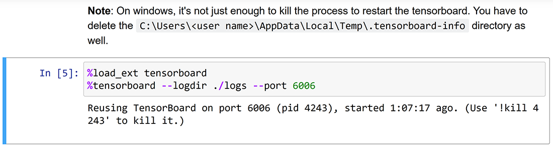
Figure 14.1 Jupyter magic commands in a notebook cell

You might notice that this is not typical Python syntax. Commands such as these that start with a % sign are known as Jupyter magic commands. Remember that Jupyter is the name of the Python library that is producing notebooks that we have our code in. You can see a list of such commands at http://mng.bz/BMd1. The first command loads the TensorBoard Jupyter notebook extension. The second command instantiates a TensorBoard with the provided logging directory (--logdir) argument and a port (--port) argument. If you don’t specify a port, TensorBoard will run on 6006 (or the first unused port greater than 6006) by default. Figure 14.2 shows how the TensorBoard looks with visualized images.

Figure 14.2 The TensorBoard visualizing logged images, displayed inline in the Jupyter notebook. You can perform various operations on images, such as adjusting brightness or contrast. Furthermore, the subdirectories to which the data is logged are shown on the left-hand panel, allowing you to easily show/hide different subdirectories for easier comparison.

Alternatively, you can also visualize the TensorBoard on a browser tab independent of the Jupyter notebook. After you run the two commands in your browser, open http://localhost:6006, which will display the TensorBoard as shown in figure 14.2. In the next section, we will see how TensorBoard can be used to track and monitor model performance as models are trained.

Exercise 1

You have a list of five batches of images in a variable called step_image_batches. Each item in the list corresponds to the first five steps of the training. You want to have these batches shown in the TensorBoard, each with the correct step value. You can name each batch as batch_0, batch_1, and so on. How would you do this?

14.2 Tracking and monitoring models with TensorBoard

With a good understanding of the data in the Fashion-MNIST data set, you will use a neural network to train a model on this data to gauge how accurately you can classify different types of apparel. You are planning to use a dense network and a convolutional neural network. You will train both these models under the same conditions (e.g., data sets) and visualize the model’s accuracy and loss on the TensorBoard.

The primary purpose served by the TensorBoard is the ability to visualize a model’s performance as it is trained. Deep neural networks are notoriously known for their long training times. There is no doubt that identifying problems with a model as early as possible pays off well. The TensorBoard plays a vital role in that. You can pipe model performance (through evaluation metrics) to be displayed in real time on TensorBoard. Therefore, you can spot any abnormal behaviors in the model before spending too much time and take necessary actions quickly.

In this section, we will compare the performance of a fully connected network and a convolutional neural network on the Fashion-MNIST data set. Let’s define a small fully connected model as the first model we want to test with this data set. It will have three layers:

• A layer with 512 neurons and ReLU activation that takes a flattened image from the Fashion-MNIST data set

• A layer with 256 neurons and ReLU activation that takes the previous layer’s output

• A layer with 10 outputs (representing the categories) that has a softmax activation

The model is compiled with sparse categorical cross-entropy loss and the Adam optimizer. Since we’re interested in the model accuracy, we add that to the list of metrics that are tracked:

from tensorflow.keras import layers, models
 
 
dense_model = models.Sequential([
    layers.Dense(512, activation='relu', input_shape=(784,)),
    layers.Dense(256, activation='relu'),
    layers.Dense(10, activation='softmax')
])
 
dense_model.compile(loss="sparse_categorical_crossentropy", optimizer='adam', metrics=['accuracy'])

With the model fully defined, we train it on the training data and evaluate it on the validation data set. First, let’s define the logging directory for the fully connected model:

log_datetimestamp_format = "%Y%m%d%H%M%S"
log_datetimestamp = datetime.strftime(
    datetime.now(), log_datetimestamp_format
)
 
dense_log_dir = os.path.join("logs","dense_{}".format(log_datetimestamp))

As before, you can see that we are not only writing to subdirectories instead of the plain flat directory, but we are also using a unique identifier that is based on the time of running. Each of these subdirectories represents what is called a run in TensorBoard terminology.

./logs/dense/run_2021-05-27-03-14-21_lr=0.01
./logs/dense/run_2021-05-27-09-02-52_lr=0.001
./logs/dense/run_2021-05-27-10-12-09_lr=0.001
./logs/dense/run_2021-05-27-14-43-12_lr=0.0005

./logs/dense/lr=0.01/2021-05-27-03-14-21
./logs/dense/lr=0.001/2021-05-27-09-02-52
./logs/dense/lr=0.001/2021-05-27-10-12-09
./logs/dense/lr=0.0005/2021-05-27-14-43-12

I would like to stress that it is important to time stamp your runs, as explained in the sidebar. This way you will have a unique folder for each run and can always go back to previous runs to compare if needed. Next, let’s generate training/validation/testing data sets using the get_train_valid_test() function. Make sure to set the flatten_ images=True:

batch_size = 64
tr_ds, v_ds, ts_ds = get_train_valid_test_datasets(
    fashion_ds, batch_size=batch_size, flatten_images=True
)

Modeling metrics to the TensorBoard is very easy. There is a special callback for the TensorBoard that you can pass during the model training/evaluation:

tb_callback = tf.keras.callbacks.TensorBoard(
    log_dir=dense_log_dir, profile_batch=0
)

Let’s discuss some of the key arguments you can pass to the TensorBoard callback. The default TensorBoard callback looks as follows:

tf.keras.callbacks.TensorBoard(
    log_dir='logs', histogram_freq=0, write_graph=True,
    write_images=False, write_steps_per_second=False, update_freq='epoch',
    profile_batch=2, embeddings_freq=0, embeddings_metadata=None, 
)

Now we will look at the arguments provided:

• log_dir—The directory to log information to. Once the TensorBoard is spun up using the log dir as this (or a parent of this) directory, the information can be visualized on the TensorBoard (defaults to 'logs').

• histogram_freq—Creates histograms of activation distribution in layers (discussed in detail later). This specifies how frequently (in epochs) these histograms need to be recorded (defaults to 0, meaning it’s disabled).

• write_graph—Determines whether to write the model as a graph to visualize on the TensorBoard (defaults to True).

• write_image—Determines whether to write model weights as an image (i.e., a heat map) to visualize the weights on the TensorBoard (defaults to False).

• write_steps_per_second—Determines whether to write the number of steps performed in a second to the TensorBoard (defaults to False).

• update_freq ('batch', 'epoch' or an integer)—Determines whether to write updates to the TensorBoard every batch (if the value is set to batch) or epoch (if value is set to epoch). Passing an integer, TensorFlow will interpret it as “write to the TensorBoard every x batches.” By default, updates will be written every epoch. Writing to the disk is expensive; therefore, writing too frequently will slow your training down.

• profile_batch (an integer or a list of two numbers)—Determines which batches to use for profiling the model. Profiling computes computational and memory profiles of the model (discussed in detail later). If an integer is passed, it will profile a single batch. If a range (i.e., a list of two numbers) is passed, it will profile batches in that range. If set to zero, profiling will not happen (defaults to 2).

• embedding_freq—If the model has an embedding layer, this parameter specifies the interval (in epochs) to visualize the embedding layer. If set to zero, this is disabled (defaults to 0).

• embedding_metadata—A dictionary that maps the embedding layer name to a file name. The file should consist of the tokens corresponding to each row in the embedding matrix (in that order; defaults to None).

Finally, we will train the model as we have done before. The only difference is that we pass tb_callback as a callback to the model:

dense_model.fit(tr_ds, validation_data=v_ds, epochs=10, callbacks=[tb_callback])

The model should reach a validation accuracy of around 85%. Now open the TensorBoard by visiting http:/ /localhost:6006. It will display a dashboard similar to figure 14.3. The dashboard will be refreshed automatically as new data appears in the log directory.

Figure 14.3 How tracked metrics are displayed on the TensorBoard. You can see the training and validation accuracy and the loss are plotted as line graphs. Furthermore, you have various controls, such as maximizing the graph, switching to a log-scale y-axis, and so on.

The TensorBoard dashboard has many controls that help users understand their models in great depth with the help of logged metrics. You can turn different runs on or off depending on what you want to analyze. For example, if you only want to look at validation metrics, you can switch off dense/train run, and vice versa. Data/train run does not affect this panel as it contains images we logged from the training data. To view them, you can click on the IMAGES panel.

Next, you can change the smoothing parameter to control the smoothness of the line. It helps to remove localized small changes in metrics and focus on global trends by having a smoother version of the line. Figure 14.4 depicts the effect of the smoothing parameter on line plots.

Figure 14.4 How the smoothing parameter changes the line plot. Here, we are showing the same line plot under different smoothing parameters. You can see how the line gets smoother as the smoothing parameter increases. The original line is shown in faded colors.

Additionally, you have other controls such as switching to a log-scale y-axis instead of a linear one. This is useful if metrics observe large changes over time. In log scale, such large changes will become smaller. You can also toggle between standard-sized plots and full-sized plots if you need to examine the graphs in more detail. Figure 14.3 highlights these controls.

After that, we will define a simple convolutional neural network and do the same. That is, we will define the network first, and then train the model while using a callback to the TensorBoard.

Let’s define the next model we will compare our fully connected network to: a convolutional neural network (CNN). Again, we are defining a very simple CNN that encompasses

• A 2D convolution layer with 32 filters with a 5 × 5 kernel, 2 × 2 strides, and ReLU activation that takes a 2D 28 × 28-sized image from the Fashion-MNIST data set

• A 2D convolution layer with 16 filters with a 3 × 3 kernel, 1 × 1 strides, and ReLU activation that takes the previous layer’s output

• A Flatten layer that will flatten the convolutional output to a 1D vector suitable for a Dense layer

• A layer with 10 outputs (representing the categories) that has a softmax activation

conv_model = models.Sequential([
    layers.Conv2D(
       filters=32, 
       kernel_size=(5,5), 
       strides=(2,2), 
       padding='same', 
       activation='relu', 
       input_shape=(28,28,1)
    ),
    layers.Conv2D(
        filters=16, 
        kernel_size=(3,3), 
        strides=(1,1), 
        padding='same', 
        activation='relu'
    ),
    layers.Flatten(),
    layers.Dense(10, activation='softmax')
])
 
conv_model.compile(
    loss="sparse_categorical_crossentropy", optimizer='adam', 
➥ metrics=['accuracy']
)
conv_model.summary()

Moving onto the model training, we will log the CNN-related metrics to a separate directory called ./logs/conv_{datetimestamp}. This way, we can plot the evaluation metrics of the fully connected network and the CNN under two separate runs. We will generate training and validation data sets and a TensorBoard callback, as we did earlier. These are then passed to the model when calling the fit() method to train the model:

log_datetimestamp_format = "%Y%m%d%H%M%S"
log_datetimestamp = datetime.strftime(
    datetime.now(), log_datetimestamp_format
)
 
conv_log_dir = os.path.join("logs","conv_{}".format(log_datetimestamp))
 
batch_size = 64
tr_ds, v_ds, ts_ds = get_train_valid_test_datasets(
    fashion_ds, batch_size=batch_size, flatten_images=False
)
 
tb_callback = tf.keras.callbacks.TensorBoard(
    log_dir=conv_log_dir, histogram_freq=2, profile_batch=0
)
 
conv_model.fit(
    tr_ds, validation_data=v_ds, epochs=10, callbacks=[tb_callback]
)

Notice the changes we have made when training the CNN. First, we do not flatten the images like we did when training the fully connected network (i.e., we set flatten_ images=False in the get_train_valid_test_datasets() function). Next, we introduce a new argument to the TensorBoard callback. We will use the histogram_freq argument to log layer activation histograms of the model during the training process. We will discuss layer activation histograms in more depth shortly. This will display the accuracy and loss metrics of both models (i.e., dense model and convolutional model) in the same graph, so they can be easily compared (figure 14.5).

Figure 14.5 Viewing metrics of both the dense model and the convolutional model. You can switch different runs off/on depending on what you want to compare.

Let’s come back to activation histograms again. Activation histograms let us visualize the neuron activation distribution of different layers as the training progresses. This is an important check that allows you to see whether or not the model is converging during the optimization, giving insights into problems in model training or data quality.

Let’s look at what these histograms show in more depth. Figure 14.6 illustrates the histograms generated for the CNN we have trained. We have plotted histograms every two epochs. Weights represented as histograms are stacked behind each other so we can easily understand how they evolved over time. Each slice in the histogram shows the weight distribution in a given layer and a given epoch. In other words, it will provide information such as “there were x number of outputs, having a value of y, approximately.”

Figure 14.6 Activation histograms displayed by the TensorBoard. These graphs indicate how the distribution of activations in a given layer changed over time (lighter ones represent more recent epochs).

Typically, if you have a vector of values, it is quite straightforward to create the histogram. For example, assume the values are [0.1, 0.3, 0.35, 0.5, 0.6, 0.61, 0.63], and say that you have four bins: [0.0, 0.2), [0.2, 0.4), [0.4, 0.6), and [0.6, 0.8). You’d get the histogram shown in figure 14.7. If you look at the line connecting the midpoints of the bars, it’s similar to what you see in the dashboard.

Figure 14.7 A histogram generated for the sequence [0.1, 0.3, 0.35, 0.5, 0.6, 0.61, 0.63]

However, computing histograms involves more complex data manipulations when data is large and sparse, like in a weight matrix. For example, computing histograms in TensorBoard involves using exponential bin sizes (as opposed to uniform bin sizes, as in the example), which gives more fine-grained bins near zero and wider bins as you move away from zero. Then it resamples these uneven-sized bins to uniformly sized bins for easier and more meaningful visualizations. The specific details of these computations are beyond the scope of this book. If you want more details, refer to http://mng.bz/d26o.

We can see in the graphs that the weights are converging to an approximate normal distribution as the training progresses. But the bias converges to a multi-modal distribution, with spikes appearing in many different places.

This section elucidated how you can use the TensorBoard for some of the primary data visualization and model performance tracking. These are vital parts of the core checkpoints you have to set up in your data science project. Visualizing data needs to be done early in your project to help you understand the data and its structure. Model performance tracking is important as deep learning models take longer to train, and you need to complete that training within a limited budget (of both time and cost). In the next section, we will discuss how we can log custom metrics to the TensorBoard and visualize them.

Exercise 2

You have a binary classification model represented by classif_model. You’d like to track precision and recall for this model in the TensorBoard. Furthermore, you’d like to visualize the activation histograms every epoch. How would you compile the model and fit it with data using the TensorBoard callback to achieve this? TensorFlow provides tf.keras.metrics.Precision() and tf.keras.metrics.Recall() to compute precision and recall, respectively. You can assume that you are logging directly to the ./logs directory. Assume that you have been provided training data (tr_ds) and validation data (v_ds) as tf.data.Dataset objects.

14.3 Using tf.summary to write custom metrics during model training

Imagine you are a PhD student researching the effects of batch normalization. Particularly, you need to analyze how the weights’ mean and standard deviation in a given layer change over time, with and without batch normalization. For this, you will use a fully connected network and log the weights’ mean and standard deviation at every step on the TensorBoard. As this is not a typical metric that you can produce using the Keras model, you will log it (for every step) during model training in a custom training loop.

In order to compare the effects of batch normalization, we need to define two different models: one without batch normalization and one with batch normalization. Both these models will have the same specifications, apart from using batch normalization. First, let’s define a model without batch normalization:

from tensorflow.keras import layers, models
import tensorflow.keras.backend as K
 
K.clear_session()
dense_model = models.Sequential([
    layers.Dense(512, activation='relu', input_shape=(784,)),    
    layers.Dense(256, activation='relu', name='log_layer'),    
    layers.Dense(10, activation='softmax')
])
 
dense_model.compile(loss="sparse_categorical_crossentropy", optimizer='adam', metrics=['accuracy'])

The model is quite straightforward and identical to the fully connected model we defined earlier. It has three layers, with 512, 256, and 10 nodes, respectively. The first two layers use ReLU activation, whereas the last layer uses softmax activation. Note that we name the second Dense layer log_layer. We will use this layer to compute the metrics we’re interested in. Finally, the model is compiled with sparse categorical cross-entropy loss, the Adam optimizer, and accuracy as metrics. Next, we define the same model with batch normalization:

dense_model_bn = models.Sequential([
    layers.Dense(512, activation='relu', input_shape=(784,)),
    layers.BatchNormalization(),
    layers.Dense(256, activation='relu', name='log_layer_bn'),
    layers.BatchNormalization(),
    layers.Dense(10, activation='softmax')
])
 
dense_model_bn.compile(
    loss="sparse_categorical_crossentropy", optimizer='adam', 
➥ metrics=['accuracy']
)

Introducing batch normalization means adding tf.keras.layers.BatchNormalization() layers between the Dense layers. We name the layer of interest in the second model as log_layer_bn, as we cannot have two layers with the same name at once.

With the models defined, our task is to compute the mean and standard deviation of weights at every step. To do that, we will observe the mean and standard deviation of the weights in the second layer of both networks (log_layer and log_layer_bn). As we have already discussed, we cannot simply pass a TensorBoard callback and expect these metrics to be available. Since the metrics we’re interested in are not commonly used, we have to do the heavy lifting and make sure the metrics are logged every step.

We will define a train_model() function, to which we can pass the defined model and train it on the data. While training, we will compute the mean and the standard deviation of the weights in every step and log that to the TensorBoard (see the next listing).

Listing 14.2 Writing a tf.summary object while training the model in a custom loop

def train_model(model, dataset, log_dir, log_layer_name, epochs):    
    
    writer = tf.summary.create_file_writer(log_dir)                        ❶
    step = 0
    
    with writer.as_default():                                              ❷
        
        for e in range(epochs):
            print("Training epoch {}".format(e+1))
            for batch in tr_ds:
                
                model.train_on_batch(*batch)                               ❸
                
                weights = model.get_layer(log_layer_name).get_weights()[0] ❹
                                
                tf.summary.scalar("mean_weights",np.mean(np.abs(weights)), ❺
➥ step=step)                                                              ❺
                tf.summary.scalar("std_weights", np.std(np.abs(weights)),  ❺
➥ step=step)                                                              ❺
                
                writer.flush()                                             ❻
                
                step += 1
            print('	Done')
    
    print("Training completed
")

❶ Define the writer.

❷ Open the writer.

❸ Train with one batch.

❹ Get the weights of the layer. It’s a list of arrays [weights, bias] in that order. Therefore, we’re only taking the weights (index 0).

❺ Log mean and std of absolute weights (which are two scalars for a given epoch).

❻ Flush to the disk from the buffer.

Note how we open a tf.summary.writer() and then log the metrics in every step using the tf.summary.scalar() call. We are giving the metrics meaningful names to make sure we know which is which when visualizing them on the TensorBoard. With the function defined, we call it for the two different models we have compiled:

batch_size = 64
tr_ds, _, _ = get_train_valid_test_datasets(
    fashion_ds, batch_size=batch_size, flatten_images=True
)
train_model(dense_model, tr_ds, exp_log_dir + '/standard', "log_layer", 5)
 
tr_ds, _, _ = get_train_valid_test_datasets(
    fashion_ds, batch_size=batch_size, flatten_images=True
)
train_model(dense_model_bn, tr_ds, exp_log_dir + '/bn', "log_layer_bn", 5)

Note that we are specifying different logging subdirectories to make sure the two models that appear are different runs. After running this, you will see two new additional sections called mean_weights and std_weights (figure 14.8). It seems that the mean and variance of weights change more drastically when batch normalization is used. This could be because, as batch normalization introduces explicit normalization between layers, weights of layers have more freedom to move around.

Figure 14.8 The mean and standard deviation of weights plotted in the TensorBoard

The next section expands on how the TensorBoard can be used to profile models and provides in-depth analysis of how time spent and memory are consumed when models are executed.

Exercise 3

You are planning to compute Fibonacci numbers (i.e., 0, 1, 1, 2, 3, 5, 8, 13, 21, 34, 55, etc.), where the n^th number x_n is given by x_n = x_{n - 1} + x_{n - 2}. Write a code to compute the Fibonacci series for 100 steps and plot it as a line graph in TensorBoard. You can use the name “fibonacci” as the name for the metric.

14.4 Profiling models to detect performance bottlenecks

You are starting off as a data scientist at a bio-tech company that is identifying endangered flower species. One of the previous data scientists developed a model, and you are continuing that work. First, you want to determine if there are any performance bottlenecks. To analyze such issues, you plan to use the TensorBoard profiler. You will be using a smaller flower data set for the purpose of training the model so that the profiler can capture various computational profiles.

We start with the model in listing 14.3. It is a CNN model that has four convolutional layers, with pooling layers in between and three fully connected layers, including a final softmax layer with 17 output classes.

Listing 14.3 The CNN model available to you

def get_cnn_model():
    
    conv_model = models.Sequential([                                ❶
        layers.Conv2D(                                              ❷
            filters=64, 
            kernel_size=(5,5), 
            strides=(1,1), 
            padding='same', 
            activation='relu', 
            input_shape=(64,64,3)
        ),
        layers.BatchNormalization(),                                ❸
        layers.MaxPooling2D(pool_size=(3,3), strides=(2,2)),        ❹
        layers.Conv2D(                                              ❺
            filters=128, 
            kernel_size=(3,3), 
            strides=(1,1), 
            padding='same', 
            activation='relu'
        ),
        layers.BatchNormalization(),                                ❺
        layers.Conv2D(                                              ❺
            filters=256, 
            kernel_size=(3,3), 
            strides=(1,1), 
            padding='same', 
            activation='relu'
        ),
        layers.BatchNormalization(),                                ❺
        layers.Conv2D(                                              ❺
            filters=512, 
            kernel_size=(3,3), 
            strides=(1,1), 
            padding='same', 
            activation='relu'
        ),
        layers.BatchNormalization(),                                ❺
        layers.AveragePooling2D(pool_size=(2,2), strides=(2,2)),    ❻
        layers.Flatten(),                                           ❼
        layers.Dense(512),                                          ❽
        layers.LeakyReLU(),                                         ❽
        layers.LayerNormalization(),                                ❽
        layers.Dense(256),                                          ❽
        layers.LeakyReLU(),                                         ❽
        layers.LayerNormalization(),                                ❽
        layers.Dense(17),                                           ❽
        layers.Activation('softmax', dtype='float32')               ❽
    ])
    return conv_model

❶ Define a Keras model using the sequential API.

❷ Define the first convolutional layer that takes a 64 × 64 × 3-sized input.

❸ A batch normalization layer

❹ A max pooling layer

❺ A series of alternating convolution and batch normalization layers

❻ An average pooling layer that marks the end of convolutional/pooling layers

❼ Flatten the output of the last pooling layer.

❽ A set of Dense layers (with leaky ReLU activation), followed by a layer with softmax activation

The data set we’re going to use is a flower data set found at https://www.robots.ox.ac.uk/~vgg/data/flowers, specifically, the 17-category data set. It has a single folder with images of flowers, and each image filename has a number. The images are numbered in such a way that, when sorted by the filename, the first 80 images belong to class 0, the next 80 images belong to class 1, and so on. You have been provided the code to download the data set in the notebook Ch14/14.1_Tensorboard.ipynb, which we will not discuss here. Next, we will write a simple tf.data pipeline to create batches of data by reading these images in:

def get_flower_datasets(image_dir, batch_size, flatten_images=False):
 
    # Get the training dataset, shuffle it, and output a tuple of (image, 
➥ label)
    dataset = tf.data.Dataset.list_files(
        os.path.join(image_dir,'*.jpg'), shuffle=False
    )
 
    def get_image_and_label(file_path):
 
        tokens = tf.strings.split(file_path, os.path.sep)
        label = (
            tf.strings.to_number(
                tf.strings.split(
                    tf.strings.split(tokens[-1],'.')[0], '_'
                )[-1]
            ) -1
        )//80
 
        # load the raw data from the file as a string
        img = tf.io.read_file(file_path)
        img = tf.image.decode_jpeg(img, channels=3)
 
        return tf.image.resize(img, [64, 64]), label
 
    dataset = dataset.map(get_image_and_label).shuffle(400)
 
    # Make the validation dataset the first 10000 data
    valid_ds = dataset.take(250).batch(batch_size)
    # Make training dataset the rest
    train_ds = dataset.skip(250).batch(batch_size)
    )
 
    return train_ds, valid_ds

Let’s analyze what we’re doing here. First, we read the files which have a .jpg extension from a given folder. Then we have a nested function called get_image_and_label(), which takes a file path of an image and produces the image by reading it from the disk and the label. The label can be computed by

• Extracting the image ID

• Subtracting 1 (i.e., to make IDs zero-based indices) and dividing by 80

After that, we shuffle the data and take the first 250 as validation data and the rest as training data. Next, we use these functions defined and train the CNN model while creating various computational profiles of the model. In order for the profiling to work, you need two main prerequisites:

• Install the Python package tensorboard_plugin_profile.

• Install libcupti, the CUDA Profiling Toolkit Interface.

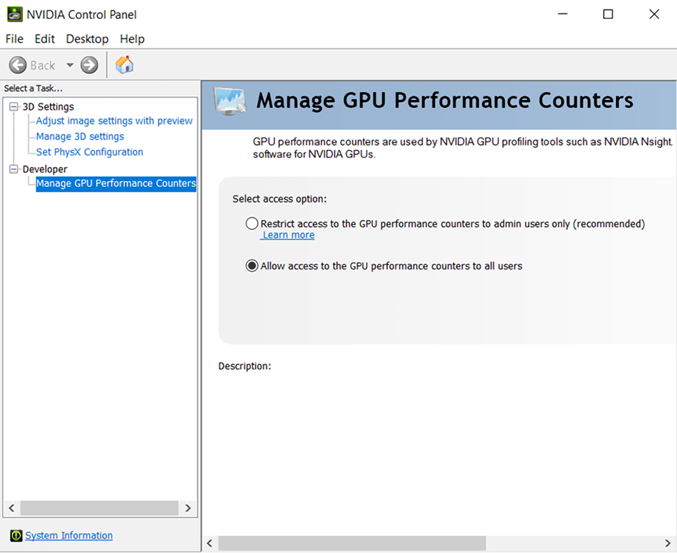
Make sure you have libcupti installed properly in the environment you are using (e.g., Ubuntu or Windows). Otherwise, you will not see the expected results. Then, to enable profiling, all you need to do is pass the argument profile_batch to the TensorBoard callback. The value is a list of two numbers: the starting step and the ending step. Profiling is typically done across a span of several batches and therefore requires a range as the value. However, profiling can be done for a single batch too:

batch_size = 32
tr_ds, v_ds = get_flower_datasets(
    os.path.join(
        'data', '17flowers','jpg'), batch_size=batch_size, 
➥ flatten_images=False
)
 
tb_callback = tf.keras.callbacks.TensorBoard(
    log_dir=profile_log_dir, profile_batch=[10, 20]
)
 
conv_model.fit(
    tr_ds, validation_data=v_ds, epochs=2, callbacks=[tb_callback]
)

Once the training finishes, you can view the results on the TensorBoard. TensorBoard provides a large collection of valuable information and insights on model performance. It breaks down the computation into smaller subtasks and provides fine-grained computational time decomposition based on those subtasks. Furthermore, TensorBoard provides recommendations on where there is room for improvement (figure 14.10). Let’s now delve into more details about the information provided on this page.

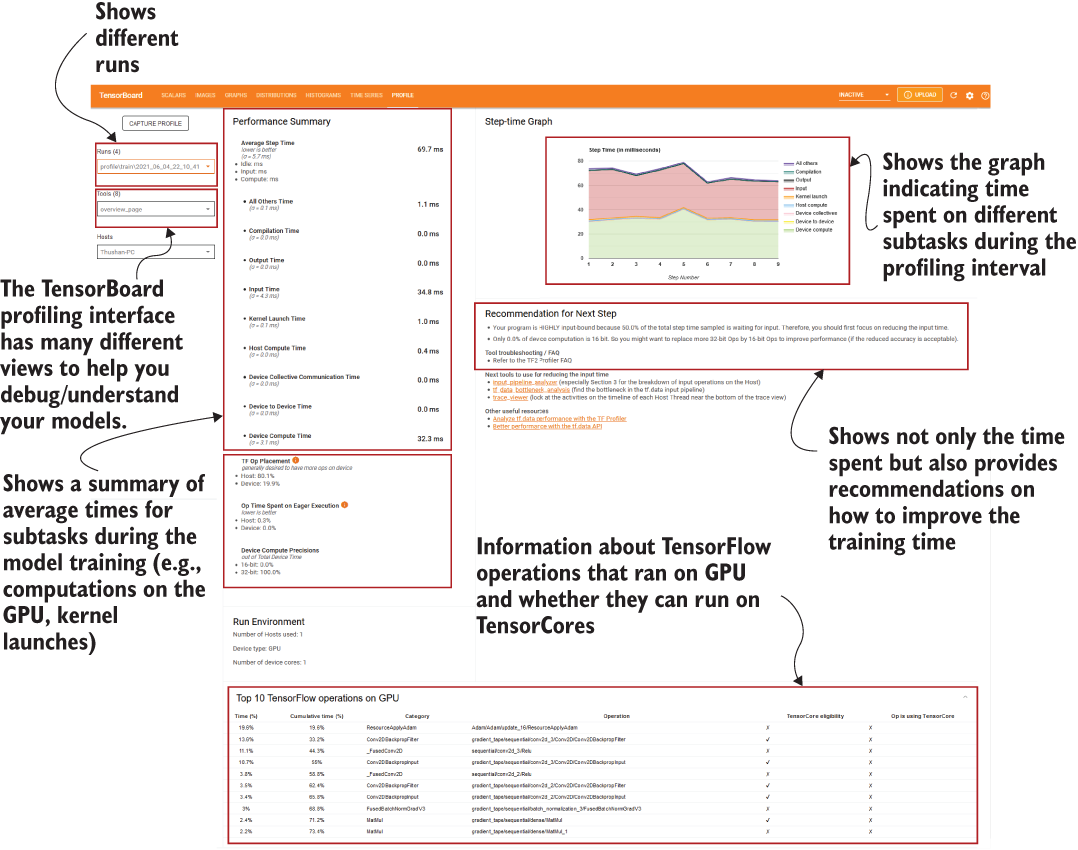
Figure 14.10 TensorBoard profiling interface. It gives a valuable collection of information on various subtasks involved in running models on the GPU. In addition, it provides recommendations on how to improve the performance of the models.

The average step time is a summation of several smaller tasks:

• Input time—Time spent on reading data-related operations (e.g., tf.data.Dataset operations).

• Host compute time—Model-related computations done on the host (e.g., CPU).

• Device-to-device time—To run things on the GPU, data first needs to be transferred to the GPU. This subtask measures the time taken for such transfers.

• Kernel launch time—For the GPU to execute operations on the transferred data, the CPU needs to launch the kernels for the GPU. A kernel encapsulates a primitive computation performed on data (e.g., matrix multiplication). This measures the time taken for launching kernels.

• Device compute time—Model-related computations that happen on the device (e.g., GPU).

• Device collective communication time—Relates to time spent on communicating in multi-device (e.g., multiple GPUs) or multi-node environments.

• All the other times (e.g., compilation time, output time, all other remaining time).

Here we can see that the most time is spent on device computations. This is, in a way, good, as it means that most computations happen on the GPU. The next-biggest time consumer is the input time. This makes sense as we are not using any optimizations for our tf.data pipeline and it is a highly disk-bound pipeline as images are read from the disk.

Then, right below that, you can see some more information. Close to 80% of the TensorFlow ops were placed on this host, whereas only 20% ran on the GPU. Furthermore, all the operations were 32-bit operations, and none were 16-bit; 16-bit (half-precision floating point) operations run faster and save a lot of memory compared to 32-bit (single-precision floating point) data types. GPUs and Tensor Processing Units (TPUs) are optimized hardware that can run 16-bit operations much faster than 32-bit operations. Therefore, they must be incorporated whenever possible. Having said that, we must be careful how we use 16-bit operations, as incorrect usage can hurt model performance (e.g., model accuracy) significantly. Incorporating 16-bit operations along with 32-bit operations to train the model is known as mixed precision training.

If you look at the recommendation section, you can see two main recommendations:

• Optimize the input data pipeline.

• Utilize more 16-bit operations in model training.

Let’s see how we can use these recommendations to reduce model training time.

14.4.1 Optimizing the input pipeline

To optimize the data pipeline, we will introduce two changes to our get_flower_ datasets() function:

• Use data prefetching to avoid the model having to wait for the data to become available.

• Use the parallelized map function when calling the get_image_and_label() function.

In terms of how these changes are reflected in the code, they are minor changes. In the following listing, the changes are in bold.

Listing 14.4 The function generating training/validation data sets from flower data set

def get_flower_datasets(image_dir, batch_size, flatten_images=False):
 
    dataset = tf.data.Dataset.list_files(
        os.path.join(image_dir,'*.jpg'), shuffle=False          ❶
    )
 
    def get_image_and_label(file_path):                         ❷
 
        tokens = tf.strings.split(file_path, os.path.sep)       ❸
        label = (tf.strings.to_number(
            tf.strings.split(
                tf.strings.split(tokens[-1],'.')[0], '_')[-1]   ❸
            ) - 1
        )//80
 
        img = tf.io.read_file(file_path)                        ❹
        img = tf.image.decode_jpeg(img, channels=3)             ❹
 
        return tf.image.resize(img, [64, 64]), label
 
    dataset = dataset.map(
        get_image_and_label,
        num_parallel_calls=tf.data.AUTOTUNE                     ❺
    ).shuffle(400)
 
    # Make the validation dataset the first 10000 data
    valid_ds = dataset.take(250).batch(batch_size)
    # Make training dataset the rest
    train_ds = dataset.skip(250).batch(batch_size).prefetch(
        tf.data.experimental.AUTOTUNE                           ❻
    )
 
    return train_ds, valid_ds

❶ Get the training data set, shuffle it, and output a tuple of (image, label).

❷ Define a function to get the image and the label given a file name.

❸ Get the tokens in the file path and compute the label from the image ID.

❹ Read the image and convert to a tensor.

❺ Parallelize the map function.

❻ Incorporate prefetching.

To parallelize the dataset.map() function, we add the num_parallel_calls=tf.data .AUTOTUNE argument, which will cause TensorFlow to execute the map function in parallel, where the number of threads will be determined by the workload carried out by the host at the time. Next, we invoke the prefetch() function on the data after batching to make sure the model training is not hindered by waiting for the data to become available.

Next, we will set a special environment variable called TF_GPU_THREAD_MODE. To understand the effects of this variable, you first need to grok how GPUs execute instructions at a high level. When you run deep learning models on a machine with a GPU, most of the data-parallel operations (i.e., operations that can be parallelly executed on data) get executed on the GPU. But how do data and instructions get to the GPU? Assume use of a GPU to execute an element-wise multiplication between two matrices. Since individual elements can be multiplied in parallel, this is a data-parallel operation. To execute this operation (defined as a set of instructions and referred to as a kernel) on the GPU, the host (CPU) first needs to launch the kernel in order for the GPU to use that function on data. Particularly, a thread in the CPU (a modern Intel CPU has around two threads per core) will need to trigger this. Think about what will happen if all the threads in the CPU are very busy. In other words, if there are a lot of CPU-bound operations happening (e.g., doing lot of reads from the disk), it can create CPU contention, causing these GPU kernel launches to be delayed. This, in turn, delays code getting executed on the GPU. With the TF_GPU_THREAD_MODE variable, you can alleviate the delays on the GPU caused by CPU contention. More concretely, this variable controls how CPU threads are allocated to launch kernels on the GPU. It can take three different values:

• Global—There is no special preference as to how threads are allocated for the different processes (default).

• gpu_private—A number of dedicated threads are allocated to launch kernels for the GPU. This way, kernel launch will not be delayed, even when a CPU is executing a significant load. If there are multiple GPUs, they will have their own private threads. The number of threads defaults to two and can be changed by setting the TF_GPU_THREAD_COUNT variable.

• shared—Same as gpu_private, except in multi-GPU environments, a pool of threads will be shared between the GPUs.

We will set this variable to gpu_private. We will keep the number of dedicate threads to two, so it will not create the TF_GPU_THREAD_COUNT variable.

It is important to restart the notebook server after changing environment variables in your operating system or the conda environment. Refer to the following sidebar for more details.

We introduced three optimizations to our tf.data pipeline:

• Prefetching batches of data

• Using the parallelized map() function instead of the standard map() function

• Using dedicated kernel launch threads by setting TF_GPU_THREAD_MODE=gpu_ private

14.4.2 Mixed precision training

As explained earlier, mixed precision training refers to employing a combination of 16-bit and 32-bit operations in model training. For example, the trainable parameters (i.e., variables) are kept as 32-bit floating point values and operations (e.g., matrix multiplication) and produce 16-bit floating point outputs.

In Keras, it’s very easy to enable mixed precision training. You simply import the mixed_precision namespace from Keras and create a policy that uses mixed precision data types by passing mixed_float16. Finally, you set it as a global policy. Then, whenever you define a new model, it will use this policy to determine the data types for the model:

from tensorflow.keras import mixed_precision
policy = mixed_precision.Policy('mixed_float16')
mixed_precision.set_global_policy(policy)

Let’s redefine the CNN model we defined and do a quick check on data types to understand how this new policy has changed the model data types:

conv_model = get_cnn_model()

Now we will pick a layer and check the data types of the inputs/internal parameters (e.g., trainable weights) and outputs:

print("Input to the layers have the data type: {}".format(
    conv_model.get_layer("conv2d_1").input.dtype)
)
print("Variables in the layers have the data type: {}".format(
    conv_model.get_layer("conv2d_1").trainable_variables[0].dtype)
)
print("Output of the layers have the data type: {}".format(
    conv_model.get_layer("conv2d_1").output.dtype)
)

This will print

Input to the layers have the data type: <dtype: 'float16'>
Variables in the layers have the data type: <dtype: 'float32'>
Output of the layers have the data type: <dtype: 'float16'>

As you can see, the inputs and outputs have the float16 data type, whereas the variables have the float32 type. This is a design principle incorporated by mixed precision training. The variables are kept as type float32 to make sure the precision is preserved as the weights are updated.

With that, rerun the model training:

batch_size = 32
tr_ds, v_ds = get_flower_datasets(
    os.path.join('data', '17flowers','jpg'), batch_size=batch_size, 
➥ flatten_images=False
)
 
# This tensorboard call back does the following
# 1. Log loss and accuracy
# 2. Profile the model memory/time for 10  batches
tb_callback = tf.keras.callbacks.TensorBoard(
    log_dir=profile_log_dir, profile_batch=[10, 20]
)
 
conv_model.fit(
    tr_ds, validation_data=v_ds, epochs=2, callbacks=[tb_callback]
)

After running the model training with the various optimization steps that we introduced, we can compare the results by changing the run on the TensorBoard. For example, we show a side-by-side comparison of the elements on the overview page with and without optimizations. We can see that the time has reduced significantly after introducing the tf.data pipeline-related optimizations (figure 14.11).

Figure 14.11 Side-by-side comparison of the profiling overview with and without data- and model-related optimizations. We can see a significant reduction of the input time after introducing the optimizations.

You might be thinking that the device compute time has not gone down much after incorporating the 16-bit operations. The largest benefit of using 16-bit operations is in the memory consumption of the GPU. The TensorBoard provides a separate view called the memory profile to analyze the memory profile of the model (figure 14.12). You can use this view to analyze memory bottlenecks or memory leaks of the model.

Figure 14.12 Memory profile with and without the optimizations. The difference from using 16-bit operations is very clear, as it has reduced the memory consumption of the model significantly.

You can clearly see how the memory requirements have taken a plunge after incorporating mixed precision training. The model’s appetite for memory has gone down by approximately 76% when mixed precision training is used (from 5.48 GB to 1.25 GB).

The graph specifically refers to two types of memory: heap and stack. These are fundamental memory spaces used by programs to keep track of variables a function calls when a program is executed. From these, the heap will help us to learn about memory usage patterns or memory-related issues, as that’s where various objects and variables created during program execution are kept. For example, if memory leaks are present, you will see an increasing amount of memory used by the heap. Here, we can see that the memory usage is quite linear and can assume that there are no significant memory leaks. You can read more about heaps and stacks in the sidebar on the next page.

We also can see fine-grained details about which operations used how much memory. For example, we know that the main bottleneck of a CNN is the first Dense layer after a series of convolutional/pooling layers. Table 14.1 confirms that. That is, it shows that the Dense layer, with a shape of [115200, 512] (i.e., first Dense layer), uses the most memory.

Table 14.1 Memory breakdown table. The table shows the memory usage of various TensorFlow operations along with their data shape.

Finally, you have the trace viewer. This gives a longitudinal view of how various operations were executed on the CPU or GPU and how much time it took. This gives a very detailed view of when and how various operations were scheduled and executed.

On your left, you can see what was executed on your CPU versus on the GPU. For example, you can see that most model-related operations (e.g., convolution) were executed on the GPU, whereas tf.data operations (e.g., decoding images) were executed on the GPU. You can also note that the trace viewer shows GPU private threads separately.

TensorBoard has far more uses than what we have listed here. To know more about these, please refer the following sidebar.

In the next section, we will discuss how we can visualize and interact with word vectors on the TensorBoard.

Exercise 4

You have a model that you have already profiled. You have seen the following overview of times:

• Input time: 1.5 ms

• Device compute time: 6.7 ms

• Kernel launch time: 9.8 ms

• Output time: 10.1 ms

• Host compute time: 21.2 ms

For this scenario, assume a time recorded more than 5 ms is an opportunity for improvement. List three code/environment change recommendations to improve the model performance.

14.5 Visualizing word vectors with the TensorBoard

You are working as an NLP engineer for a movie recommendation company and have been tasked with developing a movie recommendation model that can be trained on small devices. To reduce the training overhead, one of the techniques used is using pretrained word vectors and freezing them (i.e., not training them). You think GloVe word vectors will give a good initial point and plan to use them. But before that, you have to make sure the vectors capture the semantics/relationships in the movie-specific terminology/words adequately. For that, you need to visualize word vectors for these words on TensorBoard and analyze whether GloVe vectors represent sensible relationships between words.

The first thing we need to do is download the GloVe word vectors. You have been provided the code to download GloVe vectors in the notebook, and it is very similar to how we have downloaded datasets in the past. Therefore, we will not discuss the download in detail. The GloVe word vectors are obtained from https://nlp.stanford.edu/projects/glove/. There are several different versions of GloVe vectors; they have different dimensionalities and vocabulary sizes:

• Trained on Wikipedia 2014 + Gigaword 5 data sets with 6 billion tokens; 400,000 vocabulary; uncased tokens; and 50D, 100D, 200D, and 300D vectors

• Trained on the Common Crawl data set with 42 billion tokens, 1,900,000 vocabulary, uncased tokens, and 300D vectors

• Trained on the Common Crawl data set with 840 billion tokens, 2,200,000 vocabulary, cased tokens, and 300D vectors

• Trained on the Twitter data set with 2 billion tweets; 27 billion tokens; 1,200,000 vocabulary; uncased tokens; and 25D, 50D, 100D, and 200D vectors

We will use the 50-dimensional word vectors from the first category (which is the smallest). A 50-dimensional word vector will have 50 values in each word vector designated for each token in the corpus. Once the data is extracted by running the code in the notebook, you will see a file with the name glove.6B.50d.txt in the data folder. Let’s load that as a pandas DataFrame using the pd.read_csv() function:

df = pd.read_csv(
    os.path.join('data', 'glove.6B.50d.txt'), 
    header=None, 
    index_col=0, 
    sep=None, 
    error_bad_lines=False, 
    encoding='utf-8'
)
df.head()

This will return table 14.2. Now we will download the IMDB movie reviews data set (https://ai.stanford.edu/~amaas/data/sentiment/). Since this data set is readily available as a TensorFlow data set (through the tensorflow_datasets library), we can use that:

review_ds = tfds.load('imdb_reviews')
train_review_ds = review_ds["train"]

Once we download the data, we will create a corpus that contains all the reviews (text) in the training set as a list of strings:

corpus = []
for data in train_review_ds:      
    txt = str(np.char.decode(data["text"].numpy(), encoding='utf-8')).lower()
    corpus.append(str(txt))

Next, we want to get the most common 5,000 words in this corpus so that we can compare the GloVe vectors of these common words to see if they contain sensible relationships. To get the most common words, we will use the built-in Counter object. The Counter object counts the frequencies of the words in the vocabulary:

from collections import Counter
 
corpus = " ".join(corpus)
 
cnt = Counter(corpus.split())
most_common_words = [w for w,_ in cnt.most_common(5000)]
print(cnt.most_common(100))

This will print

[('the', 322198), ('a', 159953), ('and', 158572), ('of', 144462), ('to', 
➥ 133967), ('is', 104171), ('in', 90527), ('i', 70480), ('this', 69714), 
➥ ('that', 66292), ('it', 65505), ('/><br', 50935), ('was', 47024), 
➥ ('as', 45102), ('for', 42843), ('with', 42729), ('but', 39764), ('on', 
➥ 31619), ('movie', 30887), ('his', 29059), 
➥ ... ,
➥ ('other', 8229), ('also', 8007), ('first', 7985), ('its', 7963), 
➥ ('time', 7945), ('do', 7904), ("don't", 7879), ('me', 7722), ('great', 
➥ 7714), ('people', 7676), ('could', 7594), ('make', 7590), ('any', 
➥ 7507), ('/>the', 7409), ('after', 7118), ('made', 7041), ('then', 
➥ 6945), ('bad', 6816), ('think', 6773), ('being', 6390), ('many', 6388), 
➥ ('him', 6385)]

With both the GloVe vectors and the corpus containing the most common 5,000 words in the IMDB movie reviews data set, we find the common tokens between the two sets for visualization:

df_common = df.loc[df.index.isin(most_common_words)]

This will give a list of roughly 3,600 tokens that appear in both sets.

Next, we can visualize these vectors on the TensorBoard. To reiterate, word vectors are numerical representations of tokens in a given corpus. The specialty of these word vectors (as opposed to one-hot encoding words) is that they capture the semantics of words. For example, if you compute the distance between the word vector of “cat” and “dog,” they will be a lot closer than “cat” and “volcano.” But when analyzing relationships between a larger set of tokens, we prefer a visual aid. It would be great if there was a way to visualize these word vectors on a 2D or 3D plane, which is much easier to visualize and understand. There are dimensionality-reduction algorithms such as Principal Component Analysis (PCA) (http://mng.bz/PnZw) or t-SNE (https://distill.pub/2016/misread-tsne/) that can achieve this. The specific algorithms used for this are out of scope for this book. The good news is that with TensorBoard, you can do this. TensorBoard can map these high-dimensional vectors to a smaller projection space. To do that, we have to first load these weights as a TensorFlow variable and then save it to the disk as a TensorFlow checkpoint. Then we also save the words or tokens as a new file, with one token per line, corresponding to each vector in the set of word vectors we just saved. With that, you can visualize the word vectors on the TensorBoard (see the next listing).

Listing 14.5 Visualizing word vectors on TensorBoard

from tensorboard.plugins import projector
 
log_dir=os.path.join('logs', 'embeddings')
weights = tf.Variable(df_common.values)                          ❶
 
checkpoint = tf.train.Checkpoint(embedding=weights)              ❷
checkpoint.save(os.path.join(log_dir, "embedding.ckpt"))         ❷
 
with open(os.path.join(log_dir, 'metadata.tsv'), 'w') as f:      ❸
    for w in df_common.index:
        f.write(w+'
')
        
 
config = projector.ProjectorConfig()                             ❹
embedding = config.embeddings.add()
embedding.metadata_path = 'metadata.tsv'                         ❺
projector.visualize_embeddings(log_dir, config)

❶ Create a tf.Variable with the embeddings we captured.

❷ Save the embeddings as a TensorFlow checkpoint.

❸ Save the metadata (a TSV file), where each word corresponding to the embeddings is appended as a new line.

❹ Create a configuration specific to the projector and embeddings (details are discussed in the text).

❺ Set the metadata path so that TensorBoard can incorporate that in the visualization.

To visualize the word vectors from the saved TensorFlow checkpoint and the metadata (i.e., tokens corresponding to the word vectors saved), we use the tensorboard.plugins .projector object. We then define a ProjectorConfig object and an embedding config. We will keep them with the default configurations, which suit our problem. When config.embeddings.add() is invoked, it will generate an embedding config (of type EmbeddingInfo object) with default configuration. The ProjectorConfig contains information such as the following:

• model_checkpoint_directory—The directory to which the checkpoint containing embeddings was saved

The EmbeddingInfo contains

• tensor_name—If a special tensor name was used for embeddings

• metadata_path—The path to a TSV file that contains the labels of the embeddings

To see a full list of available configurations, refer to the file at http://mng.bz/J2Zo. In its current state, the projector’s config does not support a lot of customizations. For this reason, we will keep them as default. One config we will set in the EmbeddingInfo config is the metadata_path. We will set the metadata_path to the file containing the tokens and finally pass it to the projecter.visualize_embeddings() function. We give it a logging directory, and the projector will automatically detect the TensorFlow checkpoint and load it.

We’re all good to go. On your notebook, execute the following line to bring up the TensorBoard:

%tensorboard --logdir logs/embeddings/ --port 6007

To visualize word vectors, they need to be in the exact directory the --logdir is pointing to (i.e., not in a nested folder). Therefore, we need a new TensorBoard server. This line will open a new TensorBoard server on port 6007. Figure 14.13 depicts what is displayed in the TensorBoard.

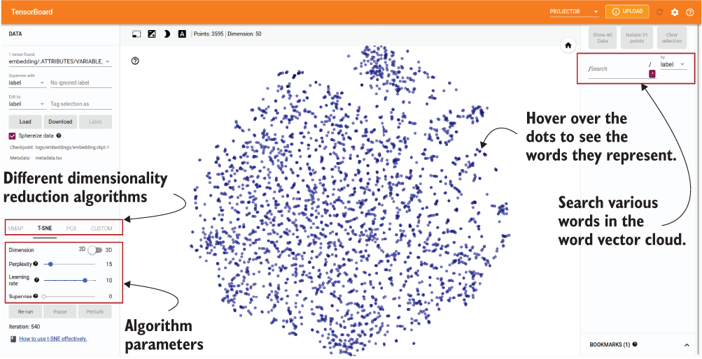
Figure 14.13 The word vector view on the TensorBoard. You have the ability to pick which dimensionality-reduction algorithm (along with parameters) to use in order to get a 2D or 3D representation of the word vectors. Hovering over the dots in the visualization will show the word represented by the dot.

You can hover over the dots shown in the visualization, and they will show which word in the corpus they represent. You have the ability to visualize the word vectors in a 2D or a 3D space by toggling the dimensionality controller. You might be wondering about the word vectors that we chose. They initially had 50 dimensions—how can we visualize such high-dimensional data in a 2D or 3D space? There’s a suite of dimensionality-reduction algorithms that can do this for us. A few examples are t-SNE (http://mng.bz/woxO), PCA (principal component analysis; http://mng.bz/ZAmZ), and UMAP (Uniform Manifold Approximation and Projection; https://arxiv.org/pdf/1802.03426.pdf). Refer to the accompanied links to learn more about these algorithms.

You can do more than a plain visualization of word vectors on the TensorBoard. You can do more detailed analysis by highlighting specific words in the visualization. For that, you can employ regular expressions. For example, the visualization shown in figure 14.14 is generated using the regular expression (?:fred|larry|mrs.|mr .|michelle|sea|denzel|beach|comedy|theater|idiotic|sadistic|marvelous| loving|gorg|bus|truck|lugosi).

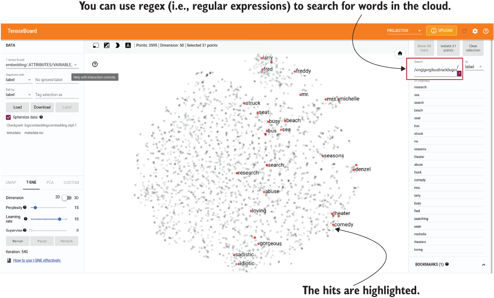
Figure 14.14 Searching words in the visualizations. You can use regular expressions to search combinations of words.

This concludes our discussion about the TensorBoard. In the next chapter, we will discuss how TensorFlow can help us to create machine learning pipelines and deploy models with ease.

Exercise 5

Instead of just the word, say you want to include a unique ID when displaying word vectors in the TensorBoard. For example, instead of the word “loving” you want to see “loving; 218,” where 218 is the unique ID given to the word. To do this, you need to change what’s written to the metadata.tsv file. Instead of just the word, write an incrementing ID separated by a semicolon on each line. For example, if the words are [“a”, “b”, “c”], in that order, then the new lines should be [“a;1”, “b;2”, “c;3”]. How would you make changes?

Summary

• TensorBoard is a great visualization aid for visualizing data (e.g., images) and tracking model performance in real time.

• When building models with Keras, you can use the convenient tf.keras.callbacks.TensorBoard() callback to log model performance, layer activation histograms, and much more.

• If you have custom metrics that you want to log to the TensorBoard, you can use the corresponding data type in the tf.summary namespace (e.g., use tf.summary.scalar() if you want to log a scalar value, like model accuracy over time).

• Each session where you log information to the TensorBoard is called a run. You should incorporate a readable and robust naming convention for the different runs. A good naming convention should capture major changes you did and the date/time the run was executed.

• TensorBoard Profile provides a diverse collection of profiling (using libcupti library by NVIDIA) results such as time taken by various subtasks during model training (e.g., device compute time, host compute time, input time, etc.), memory used by the model, and a sequential view of when and how various operations are carried out.

• TensorBoard is a great tool for visualizing high-dimensional data like images and word vectors.

Answers to exercises

Exercise 1

image_writer = tf.summary.create_file_writer(image_logdir)
 
with image_writer.as_default():
    for bi, batch in enumerate(steps_image_batches):
        tf.summary.image(
            “batch_{}”.format(bi), 
            batch, 
            max_outputs=10, 
            step=bi
        )

Exercise 2

log_dir = "./logs "
 
classif_model.compile(
    loss=’binary_crossentropy', 
    optimizer=’adam’, 
    metrics=[tf.keras.metrics.Precision(), tf.keras.metrics.Recall()]
)
    
tb_callback = tf.keras.callbacks.TensorBoard(
    log_dir=log_dir, histogram_freq=1, profile_batch=0
)
 
classif_model.fit(tr_ds, validation_data=v_ds, epochs=10, callbacks=[tb_callback])

Exercise 3

 writer = tf.summary.create_file_writer(log_dir)
    
 x_n_minus_1 = 1
 x_n_minus_2 = 0
 
 with writer.as_default():        
     for i in range(100):
         x_n = x_n_minus_1 + x_n_minus_2
         x_n_minus_1 = x_n
      x_n_minus_2 = x_n_minus_1
      
      tf.summary.scalar("fibonacci", x_n, step=i)
      
      writer.flush()

Exercise 4

1. There are a lot of computations happening on the host. This could be because the device (e.g., GPU) does not have enough memory. Using mixed precision training will help to alleviate the issue. Furthermore, there might be too much non-TensorFlow code that cannot run on the GPU. For that, using more TensorFlow operations and converting such code to TensorFlow will gain speed-ups.

2. The Kernel launch time has increased. This could be because the workload is heavily CPU-bound. In this case, we can incorporate the TF_GPU_THREAD_MODE environment variable and set it to gpu_private. This will make sure there will be several dedicated threads to launch kernels for the GPU.

3. Output time is significantly high. This could be because of writing too many outputs too frequently to the disk. To solve that, we can incorporate keeping data in memory for longer and flushing it to the disk only a few times.

Exercise 5

log_dir=os.path.join('logs', 'embeddings')
 
weights = tf.Variable(df_common.values)
   checkpoint = tf.train.Checkpoint(embedding=weights)
checkpoint.save(os.path.join(log_dir, "embedding.ckpt"))
 
with open(os.path.join(log_dir, 'metadata.tsv'), 'w') as f:
    for i, w in enumerate(df_common.index):
        f.write(w+'; '+str(i)+'
')