9 Natural language processing with TensorFlow: Sentiment analysis

This chapter covers

• Preprocessing text with Python
• Analyzing text-specific attributes important for the model
• Creating a data pipeline to handle text sequences with TensorFlow
• Analyzing sentiments with a recurrent deep learning model (LSTM)
• Training the model on imbalanced product reviews
• Implementing word embeddings to improve model performance

In the previous chapters, we looked at two compute-vision-related applications: image classification and image segmentation. Image classification focuses on recognizing if an object belonging to a certain class is present in an image. Image segmentation tasks look not only at recognizing the objects present in the image, but also which pixels in the image belong to a certain object. We also anchored our discussions around learning the backbone of complex convolutional neural networks such as Inception net (image classification) and DeepLab v3 (image segmentation) models. If we look beyond images, text data is also a prominent modality of data. For example, the world wide web is teeming with text data. We can safely assume that it is the most common modality of data available in the web. Therefore, natural language processing (NLP) has been and will be a deeply rooted topic, enabling us to harness the power of the freely available text (e.g., through language modeling) and build machine learning products that can leverage textual data to produce meaningful outcomes (e.g., sentiment analysis).

NLP is a term that we give to the overarching notion that houses a plethora of tasks having to do with text. Everything from simple tasks, such as changing the case of text (e.g., converting uppercase to lowercase), to complex tasks, such as translating languages and word sense disambiguation (inferring the meaning of a word with the same spelling depending on the context) falls under the umbrella of NLP. Following are some of the notable tasks that you will experience if you enter the realm of NLP:

• Stop word removal—Stop words are uninformative words that frequent text corpora (e.g., “and,” “it,” “the,” “am,” etc.). Typically, these words add very little or nothing to the semantics (or meaning) of text. To reduce the feature space, many tasks remove stop words in early stages before feeding text to the model.

• Lemmatization—This is another technique to reduce the feature space the model has to deal with. Lemmatization will convert a given word to its base form (e.g., buses to bus, walked to walk, went to go, etc.), which reduces the size of the vocabulary and, in turn, the dimensionality of data the model needs to learn from.

• Part of speech (PoS) tagging—PoS tagging does exactly what it says: it tags every word in a given text with a part of speech (e.g., noun, verb, adjective, etc.). The Penn Treebank project provides one of the most popular and comprehensive list of PoS tags available. To see the full list, go to http://mng.bz/mO1W.

• Named entity recognition (NER)—NER is responsible for extracting various entities (e.g., Names of people/companies, geo locations, etc.) from text.

• Language modeling—Language modeling is the task of predicting the n^th word given 1, . . . , w -1^th word. Language modeling can be used to generate songs, movie scripts, and stories by training the model on relevant data. Due to the highly accessible nature of the data needed for language modeling (i.e., it does not require any labeled data), it commonly serves as a pretraining method to inject language understanding for decision-support NLP models.

• Sentiment analysis—Sentiment analysis is the task of identifying the sentiment given a piece of text. For example, a sentiment analyzer can analyze product/ movie reviews and automatically produce a score to indicate how good the product is.

• Machine translation—Machine translation is the task of converting a phrase/ sentence in a source language to a phrase/sentence in a target language. These models are trained using bilingual parallel text corpora.

It is rare that you will not come across an NLP task as a data scientist or a ML researcher. To solve NLP tasks quickly and successfully, it is important to understand processing data, standard models used, and so on.

In this chapter, you will learn how to develop a sentiment analyzer for video game review classification. You will start by exploring the data and learn about some common NLP preprocessing steps. You will also note that the data set is imbalanced (i.e., does not have a roughly equal number of samples for all the classes) and learn what can be done about that. We will then develop a TensorFlow data pipeline with which we will pipe data to our model to train. Here, you’ll encounter a new machine learning model known as a long short-term memory (LSTM) model that has made its mark in the NLP domain. LSTM models can process sequences (e.g., a sentence—a sequence of words in a particular order) by going through each element iteratively to produce some outcome at the end. In this task, the model will output a binary value (0 for negative reviews and 1 for positive reviews). While traversing the sequence, an LSTM model maintains the memory of what it has seen so far. This makes LSTM models very powerful and able to process long sequences and learn patterns in them. After the model is trained, we will evaluate it on some test data to make sure it performs well and then save it. The high-level steps we will follow to develop this model include the following:

1. Download the data. We will use a video game review corpus from Amazon.

2. Explore and clean the data. Incorporate some text cleaning steps (e.g., lemmatization) to clean the data and prepare the corpus for the modeling task.

3. Create a data pipeline to convert raw text to a numerical format understood by machine learning models.

4. Train the model on the data produced by the data pipeline.

5. Evaluate the model on validation, and test data to ensure model’s generalizability.

6. Save the trained model, and write the performance results.

9.1 What the text? Exploring and processing text

You are building a sentiment analyzer for a popular online video game store. They want a bit more than the number of stars, as the number of stars might not reflect the sentiment accurately due to the subjectivity of what a star means. The executives believe the text is more valuable than the number of stars. You’ve been asked to develop a sentiment analyzer that can determine how positive or negative a review is, given the text.

You have decided to use an Amazon video game review data set for this. It contains various reviews posted by users along with the number of stars. Text can be very noisy due to the complexity of language, spelling mistakes, and so on. Therefore, some type of preprocessing will act as the gatekeeper for producing clean data. In this section, we will examine the data and some basic statistics. Then we will perform several preprocessing steps: comprising, lowering the case (e.g., convert “John” to “john”), removing punctuation/numbers, removing stop words (i.e., uninformative words like “to,” “the,” “a,” etc.) and lemmatization (converting words to their base form; e.g., “walking” to “walk”).

As the very first step, let’s download the data set in the next listing.

Listing 9.1 Downloading the Amazon review data set

import os
import requests
import gzip
import shutil
 
# Retrieve the data
if not os.path.exists(os.path.join('data','Video_Games_5.json.gz')):      ❶
    url = 
➥ "http:/ /deepyeti.ucsd.edu/jianmo/amazon/categoryFilesSmall/Video_Games_
➥ 5.json.gz"
    # Get the file from web
    r = requests.get(url)
 
    if not os.path.exists('data'):
        os.mkdir('data')
    
    # Write to a file
    with open(os.path.join('data','Video_Games_5.json.gz'), 'wb') as f:
        f.write(r.content)
else:                                                                     ❷
    print("The tar file already exists.")
    
if not os.path.exists(os.path.join('data', 'Video_Games_5.json')):        ❸
    with gzip.open(os.path.join('data','Video_Games_5.json.gz'), 'rb') as f_in:
        with open(os.path.join('data','Video_Games_5.json'), 'wb') as f_out:
            shutil.copyfileobj(f_in, f_out)
else:
    print("The extracted data already exists")

❶ If the gzip file has not been downloaded, download it and save it to the disk.

❷ If the gzip file is located in the local disk, don’t download it.

❸ If the gzip file exists but has not been extracted, extract it.

This code will download the data to a local folder if it doesn’t already exist and extract the content. It will have a JSON file that will contain the data. JSON is a format for representing data and is predominately used to transfer data in web requests. It allows us to define data as key-value pairs. If you look at the JSON file, you will see that it has one record per line, where each record is a set of key-value pairs, and key is the column name and value is the value of that column for that record. You can see a few records extracted from the data:

{"overall": 5.0, "verified": true, "reviewTime": "10 17, 2015", 
➥ "reviewerID": "xxx", "asin": "0700026657", "reviewerName": "xxx", 
➥ "reviewText": "This game is a bit hard to get the hang of, but when you 
➥ do it's great.", "summary": "but when you do it's great.", 
➥ "unixReviewTime": 1445040000}
{"overall": 4.0, "verified": false, "reviewTime": "07 27, 2015", 
➥ "reviewerID": "xxx", "asin": "0700026657", "reviewerName": "xxx", 
➥ "reviewText": "I played it a while but it was alright. The steam was a 
➥ bit of trouble. The more they move ... looking forward to anno 2205 I 
➥ really want to play my way to the moon.", "summary": "But in spite of 
➥ that it was fun, I liked it", "unixReviewTime": 1437955200}
{"overall": 3.0, "verified": true, "reviewTime": "02 23, 2015", 
➥ "reviewerID": "xxx", "asin": "0700026657", "reviewerName": "xxx", 
➥ "reviewText": "ok game.", "summary": "Three Stars", "unixReviewTime": 
➥ 1424649600}

Next, we will further explore the data we have:

import pandas as pd
 
# Read the JSON file
review_df = pd.read_json(
    os.path.join('data', 'Video_Games_5.json'), lines=True, orient='records'
)
# Select on the columns we're interested in 
review_df = review_df[["overall", "verified", "reviewTime", "reviewText"]]
review_df.head()

The data is in JSON format. pandas provides a pd.read_json() function to read JSON data easily. When reading JSON data, you have to make sure that you set the orient argument correctly. This is because the orient argument enables pandas to understand the structure of JSON data. JSON data is unstructured compared to CSV files, which have a more consistent structure. Setting orient='records' will enable pandas to read data structured in this way (one record per line) correctly into a pandas DataFrame. Running the previous code snippet will produce the output shown in table 9.1.

Table 9.1 Sample data from the Amazon review data set

We will now remove any records that have an empty or null value in the reviewText column:

review_df = review_df[~review_df["reviewText"].isna()]
review_df = review_df[review_df["reviewText"].str.strip().str.len()>0]

As you may have already noticed, there’s a column that says whether the review is from a verified buyer. To preserve the integrity of our data, let’s only consider the reviews from verified buyers. But before that, we have to make sure that we have enough data after filtering unverified reviews. To do that, let’s see how many records there are for different values (i.e., True and False) of the verified column. For that, we will use panda’s built-in value_counts() function as follows:

review_df["verified"].value_counts()

This will return

True     332504
False    164915
Name: verified, dtype: int64

That’s great news. It seems we have more data from verified buyers than unverified users. Let’s create a new DataFrame called verified_df that only contains verified reviews:

verified_df = review_df.loc[review_df["verified"], :]

Next, out of the verified reviews, we will evaluate the number of reviews for each different rating in the overall column:

verified_df["overall"].value_counts()

This will give

5    222335
4     54878
3     27973
1     15200
2     12118
Name: overall, dtype: int64

This is an interesting finding. Typically, we want to have equal amounts of data for each different rating. But that’s never the case in the real world. For example, here, we have four times more 5-star reviews than 4-star reviews. This is known as class imbalance. Real-world data is often noisy, imbalanced, and dirty. We will see these characteristics as we look further into the data. We will circle back to the issue of class imbalance in the data when we are developing our model.

Sentiment analysis is designed as a classification problem. Given the review (as a sequence of words, for example), the model predicts a class out of a set of discrete classes. We are going to focus on two classes: positive or negative. We will make the assumption that 5 or 4 stars indicate a positive sentiment, whereas 3, 2, or 1 star mean a negative sentiment. Astute problem formulation, such as reducing the number of classes, can make the classification task easier. To do this, we can use the convenient built-in pandas function map(). map() takes a dictionary, where the key indicates the current value, and the value indicates the value the current value needs to be mapped to:

verified_df["label"]=verified_df["overall"].map({5:1, 4:1, 3:0, 2:0, 1:0})

Now let’s check the number of instances for each class after the transformation

verified_df["label"].value_counts()

which will return

1    277213
0     55291
Name: label, dtype: int64

There’s around 83% positive samples and 17% negative samples. That’s a significant discrepancy in terms of the number of samples. The final step of our simple data exploration is to make sure there’s no order in the data. To shuffle the data, we will use panda’s sample() function. sample()is technically used to sample a small fraction of data from a large data set. But by setting frac=1.0 and a fixed random seed, we can get the full data set shuffled in a random manner:

verified_df = verified_df.sample(frac=1.0, random_state=random_seed)

Finally, we will separate the inputs and labels into two separate variables, as this will make processing easier for the next steps:

inputs, labels = verified_df["reviewText"], verified_df["label"]

Next, we will focus on an imperative task, which will ultimately improve the quality of the data that is going into the model: cleaning and preprocessing the text. Here we will focus on performing the following subtasks. You will learn more details about every subtask in the coming discussion:

• Lower the case of words.

• Treat shortened forms of words (e.g., “aren’t,” “you’ll,” etc.).

• Tokenize text into words (known as tokenization).

• Remove uninformative text, such as numbers, punctuation, and stop words. Stop words are words that are frequent in text corpora but do not justify the value of their presence enough for most NLP tasks (e.g., “and,” “the,” “am,” “are,” “it,” “he,” “she,” etc.).

• Lemmatize words. Lemmatization is the process of converting words to their base-form (e.g., plural nouns to singular nouns and past-tense verbs to present-tense verbs).

To do most of these tasks, we will rely on a famous and well-known Python library for text processing known as NLTK (Natural Language Toolkit). If you have set up the development environment, you should have the NLTK library installed. But our job is not done yet. To perform some of the subtasks, we need to download several external resources provided by NLTK:

• averaged_perceptron_tagger—Identifies part of speech

• wordnet and omw-1.4-_Will be used to lemmatize (i.e., convert words to their base form)

• stopwords—Provides the list of stop words for various languages

• punkt—Used to tokenize text to smaller components (e.g., words, sentences, etc.)

Let’s first do that:

import nltk
 
nltk.download('averaged_perceptron_tagger', download_dir='nltk')
nltk.download('wordnet', download_dir='nltk')
nltk.download('omw-1.4', download_dir='nltk')
nltk.download('stopwords', download_dir='nltk')
nltk.download('punkt', download_dir='nltk')
nltk.data.path.append(os.path.abspath('nltk'))

We can now continue with our project. To understand the various preprocessing steps that’ll be laid out here, we will zoom in on a single review, which is simply a Python string (i.e., a sequence of characters). Let’s call this single review doc.

First we can convert a string to lowercase simply by calling the function lower() on a string. lower() is a Python built-in function available for strings that will convert characters in a given string to lowercase characters:

    doc = doc.lower()

Next, we will expand the "n't" to "not" if it’s present:

import re
    
doc = re.sub(pattern=r"w+n't ", repl="not ", string=doc)

To do so, we will use regular expressions. Regular expressions give us a way to match arbitrary patterns and manipulate them in various ways. Python has a built-in library to handle regular expressions, known as re. Here, re.sub() will substitute words that match a certain pattern (i.e., any sequence of alphabetical characters followed by "n't; e.g., “don’t,” “can’t”) and replace them with a string passed as repl (i.e., “not “) in the string doc. For example, “won’t” will be replaced with “not.” We do not care about the prefix “will,” as it will be removed anyway during the stop word removal we will perform later. If you’re interested, you can read more about regular expression syntax at https://www.rexegg.com/regex-quickstart.html.

We will remove shortened forms such as ’ll, ’re, ’d, and ’ve. You might notice that this will result in uncomprehensive phrases like “wo” (i.e., “won’t” becomes “wo” + “not”); we can safely ignore them. Notice that we are treating the shortened form of “not” quite differently from other shortened forms. This is because, unlike the other shortened forms, if present, “not” can have a significant impact on what a review actually conveys. We will talk about this again in just a little while:

doc = re.sub(pattern=r"(?:'ll |'re |'d |'ve )", repl=" ", string=doc)

Here, to replace the shortened forms of ’ll, ’re, ’d, and ’ve, we are again using regular expressions. Here, r"(?:'ll|'re|'d|'ve)" is a regular expression in Python that essentially identifies any occurrence of 'll/'re/'d/'ve in doc. Then we will remove any digits in doc using the re.sub() function like before:

    doc = re.sub(pattern=r"/d+", repl="", string=doc)

We will remove stop words and any punctuation as our next step. As mentioned earlier, stop words are words that appear in text but add very little value to the meaning of the text. In other words, even if the stop words are missing from the text, you’ll still be able to infer the meaning of what’s being said. The library NLTK provides a list of stop words, so we don’t have to come up with them:

from nltk.corpus import stopwords
from nltk import word_tokenize
import string
 
EN_STOPWORDS = set(stopwords.words('english')) - {'not', 'no'}
 
(doc) if w not in EN_STOPWORDS and w not in string.punctuation]  

Here, to access the stop words, all you have to do is call from nltk.corpus import stopwords and then call stopwords.words('english'). This will return a list. If you look at the words present in the list of stop words, you’ll observe almost all the common words (e.g., “I,” “you,” “a,” “the,” “am,” “are,” etc.) you’d encounter while reading a text. But as we stressed earlier, the word “not” is a special word, especially in the context of sentiment analysis. The presence of words like “no” and “not” can completely flip the meaning of a text in our case.

Also note the use of the function word_tokenize(). This is a special processing step known as tokenization. Here, passing a string to word_tokenize() returns a list, with each word being an element. Word tokenization might look very trivial for a language like English, where words are delimited by a space character or a period. But this can be a complex task in other languages (e.g., Japanese) where separation between tokens is not explicit.

Next, we have another treatment known as lemmatization. Lemmatization truncates/ stems a given word to a base form, for example, converting plural nouns to singular nouns or past tense verbs to present tense, and so on. This can be done easily using a lemmatizer object shipped with the NLTK package:

lemmatizer = WordNetLemmatizer()

Here we are downloading the WordNetLemmatizer. WordNetLemmatizer is a lemmatizer built on the well-renowned WordNet database. If you haven’t heard of WordNet, it is a famous lexical database (in the form of a network/graph) that you can utilize for tasks such as information retrieval, machine translation, text summarization, and so on. WordNet comes in many sizes and flavors (e.g., Multilingual WordNet, Non-English WordNet, etc.). You can explore more about WordNet and browse the database online at https://wordnet.princeton.edu/:

pos_tags = nltk.pos_tag(tokens)
    clean_text = [
        lemmatizer.lemmatize(w, pos=p[0].lower()) 
        if p[0]=='N' or p[0]=='V' else w 
        for (w, p) in pos_tags
    ]

By calling the function lemmatizer.lemmatize(), you can convert any given word to its base form (if it is not already in base form). But when calling the function, you need to pass in an important argument called pos. pos refers to the PoS tag (part-of-speech tag) of that word. PoS tagging is a special NLP task, where the task is to classify a given word to a PoS tag from a given set of discrete PoS tags. Here are a few examples of PoS tags:

• DT—Determiner (e.g., a, the)

• JJ—Adjective (e.g., beautiful, delicious)

• NN—Noun, singular or mass (e.g., person, dog)

• NNS—Noun, plural (e.g., people, dogs)

• NNP—Proper noun, singular (e.g., I, he, she)

• NNPS—Proper noun, plural (e.g., we, they)

• VB—Verb, base form (e.g., go, eat, walk)

• VBD—Verb, past tense (e.g., went, ate, walked)

• VBG—Verb, gerund or present participle (e.g., going, eating, walking)

• VBN—Verb, past participle (e.g., gone, eaten, walked)

• VBP—Verb, non-third-person singular present

• VBZ—Verb, third-person singular present

You can find the full list of PoS tags at http://mng.bz/mO1W. A note-worthy observation is how the tags are organized. You can see that if you consider only the first two characters of the tags, you get a broader set of classes (e.g., NN, VB), where all the nouns will be classified with NN and verbs will be classified with VB, and so on. We will use this property to make our lives easier.

Back to our code: let’s assimilate how we are using PoS tags to lemmatize words. When lemmatizing words, you have to pass in the PoS tag for the word you are lemmatizing. This is important as the lemmatization logic is different for different types of words. We will first get a list that has (<word>, <pos>) elements for the words in tokens (returned by the tokenization process). Then we iterate through the pos_tags list and call the lemmatizer.lemmatize() function with the word and the PoS tag. We will only lemmatize verbs and nouns to save computational time.

This concludes the series of steps we are incorporating to build the preprocessing workflow for our text. We will encapsulate these steps in a function called clean_ text(), as in the following listing.

Listing 9.2 Preprocessing logic for reviews in the dataset

def clean_text(doc):
    """ A function that cleans a given document (i.e. a text string)"""
    
    doc = doc.lower()                                        ❶
    doc = doc.replace("n't ", ' not ')                      ❷
    doc = re.sub(r"(?:'ll |'re |'d |'ve )", " ", doc)    ❸
    doc = re.sub(r"/d+","", doc)                             ❹
     
    tokens = [
        w for w in word_tokenize(doc) if w not in EN_STOPWORDS and w not in 
➥ string.punctuation
    ]                                                        ❺
    
    pos_tags = nltk.pos_tag(tokens)                          ❻
    clean_text = [
        lemmatizer.lemmatize(w, pos=p[0].lower())           ❼
        if p[0]=='N' or p[0]=='V' else w                    ❼
        for (w, p) in pos_tags                               ❼
    ]
 
    return clean_text

❶ Turn to lower case.

❷ Expand the shortened form n’t to “not.”

❸ Remove shortened forms like ’ll, ’re, ’d, ’ve, as they don’t add much value to this task.

❹ Remove digits.

❺ Break the text into tokens (or words); while doing that, ignore stop words from the result.

❻ Get the PoS tags for the tokens in the string.

❼ To lemmatize, get the PoS tag of each token; if it is N (noun) or V (verb) lemmatize, else keep the original form.

You can check the processing done in the function by calling it on a sample text

sample_doc = 'She sells seashells by the seashore.'
print("Before clean: {}".format(sample_doc))
print("After clean: {}".format(clean_text(sample_doc)))

which returns

Before clean: She sells seashells by the seashore.
After clean: [“sell”, “seashell”, “seashore”]

We will leverage this function along with panda’s apply function to apply this processing pipeline on each row of text that we have in our data DataFrame:

inputs = inputs.apply(lambda x: clean_text(x))

You might want to leave your computer for a while to grab a coffee or to check on your friends. It might take close to an hour to run this one-liner. The final result looks like table 9.2.

Table 9.2 Original text versus preprocessed text

Finally, to avoid overdosing on coffee or pestering your friends by running this too many times, we will save the data to the disk:

inputs.to_pickle(os.path.join('data','sentiment_inputs.pkl'))
labels.to_pickle(os.path.join('data','sentiment_labels.pkl'))

Now, we are going to define a data pipeline to transform the data to a format that is understood by the model and can be used to train and evaluate the model.

Exercise 1

Given the string s, “i-purchased-this-game-for-99-i-want-a-refund,” you’d like to replace the dash “-” with a space and then lemmatize only the verbs in the text. How would you do that?

9.2 Getting text ready for the model

You have a clean data set with text stripped of any unnecessary or unwarranted linguistic complexities for the problem we’re solving. Additionally, the binary labels have been generated from the number of stars given for each review. Before pushing ahead with the model training and evaluation, we have to do some further processing of our data set. Specifically, we will create three subsets of data—training, validation and testing—which will be used to train and evaluate the model. Next, we will look at two important characteristics of our data sets: the vocabulary size and the distribution of the sequence length (i.e., the number of words) in the examples we have. Finally, you will convert the words to numbers (or numerical IDs), as machine learning models do not understand strings but numbers.

In this section, we will further prepare the data to be consumed by the model. Right now, we have a very nice layout of processing steps to go from a noisy, inconsistent review to a simple, consistent text string that preserves the semantics of the review. But we haven’t addressed the elephant in the room! That is, machine learning models understand numerical data, not textual data. The string “not a great game” does not mean anything to a model if you present it as is. We have to further refine our data so that we end up with a number sequence instead of a word sequence. In our journey to get the data ready for the model, we will perform the following subtasks:

• Check the size of the vocabulary/word frequency after preprocessing. This will later be used as a hyperparameter of the model.

• Check the summary statistics of the sequence length (mean, median, and standard deviation). This will later be used as a hyperparameter of the model.

• Create a dictionary that will map each unique word to a unique ID (we will call this a tokenizer).

9.2.1 Splitting training/validation and testing data

A word of caution! When performing these tasks, you might inadvertently create oozing data leakages in our model. We have to make sure we perform these tasks using only the training data set and keep the validation and testing data separate. Therefore, our first goal should be separating training/validation/test data.

We know we have an imbalanced data set. Despite having an imbalanced data set, we have to make sure our model is good at identifying both positive and negative reviews. This means the data sets we’ll be evaluating on need to be balanced. To achieve this, here’s what we will do:

• Create balanced (i.e., equal count of positive and negative samples) validation and test sets

• Assign the remaining datapoints to the training set

Figure 9.1 depicts this process.

Figure 9.1 The process for splitting training/valid/test data

We will now see how we can do this in Python. First, we start by identifying the indices that correspond to positive labels and negative labels separately:

neg_indices = pd.Series(labels.loc[(labels==0)].index)
pos_indices = pd.Series(labels.loc[(labels==1)].index)

Next, we will define the size of our validation/test set as a function of train_fraction (a user-defined argument that determines how much data to leave for the training set). We will use a default value of 0.8 for the train_fraction:

n_valid = int(
    min([len(neg_indices), len(pos_indices)]) * ((1-train_fraction)/2.0)
)

It might look like a complex computation, but it is, in fact, a simple one. We will use the valid fraction as half of the fraction of data left for training data (the other half is used for the testing set). And finally, to convert the fractional value to the actual number of samples, we multiply the fraction by the smallest of counts of positive and negative samples. This way, we make sure the underrepresented class stays as the focal point during the data split. We keep the validation set and the test set equal. Therefore

n_test = n_valid

Next, we define the three sets of indices (for train/validation/test datasets) for each label type (positive and negative). We will create a funneling process to assign data points to different data sets. First, we do the following:

1. Randomly sample n_test number of indices from the negative indices (neg_ test_indices).

2. Then randomly sample n_valid indices from the remaining indices (neg_ valid_inds).

3. The remaining indices are kept as the training instances (neg_train_inds).

The same process is then repeated for positive indices to create three index sets for training/validation/test data sets:

neg_test_inds = neg_indices.sample(n=n_test, random_state=random_seed)
neg_valid_inds = neg_indices.loc[
    ~neg_indices.isin(neg_test_inds)
].sample(n=n_test, random_state=random_seed)
neg_train_inds = neg_indices.loc[
    ~neg_indices.isin(neg_test_inds.tolist()+neg_valid_inds.tolist())
]
    
pos_test_inds = pos_indices.sample(n=n_test, random_state=random_seed
)
pos_valid_inds = pos_indices.loc[
    ~pos_indices.isin(pos_test_inds)
].sample(n=n_test, random_state=random_seed)
pos_train_inds = pos_indices.loc[        
    ~pos_indices.isin(pos_test_inds.tolist()+pos_valid_inds.tolist())
]

With the negative and positive indices to slice the inputs and labels, now it’s time to create actual data sets:

tr_x = inputs.loc[
    neg_train_inds.tolist() + pos_train_inds.tolist()
].sample(frac=1.0, random_state=random_seed)
tr_y = labels.loc[
    neg_train_inds.tolist() + pos_train_inds.tolist()
].sample(frac=1.0, random_state=random_seed)
 
v_x = inputs.loc[
    neg_valid_inds.tolist() + pos_valid_inds.tolist()
].sample(frac=1.0, random_state=random_seed)
v_y = labels.loc[
    neg_valid_inds.tolist() + pos_valid_inds.tolist()
].sample(frac=1.0, random_state=random_seed)
 
ts_x = inputs.loc[
    neg_test_inds.tolist() + pos_test_inds.tolist()
].sample(frac=1.0, random_state=random_seed)
ts_y = labels.loc[
    neg_test_inds.tolist() + pos_test_inds.tolist()
].sample(frac=1.0, random_state=random_seed)

Here, (tr_x, tr_y), (v_x, v_y), and (ts_x, ts_y) represent the training, validation, and testing data sets, respectively. Here, the data sets suffixed with _x come from the inputs, and the data sets suffixed with _y come from the labels. Finally, we can wrap the logic we discussed in a single function as in the following listing.

Listing 9.3 Splitting training/validation/testing data sets

def train_valid_test_split(inputs, labels, train_fraction=0.8):
    """ Splits a given dataset into three sets; training, validation and test """
    
    neg_indices = pd.Series(labels.loc[(labels==0)].index)                   ❶
    pos_indices = pd.Series(labels.loc[(labels==1)].index)                   ❶
    
    n_valid = int(min([len(neg_indices), len(pos_indices)]) 
       * ((1-train_fraction)/2.0))                                           ❷
    n_test = n_valid                                                         ❷
    
    neg_test_inds = neg_indices.sample(n=n_test, random_state=random_seed)   ❸
    neg_valid_inds = neg_indices.loc[~neg_indices.isin(
       neg_test_inds)].sample(n=n_test, random_state=random_seed)            ❹
    neg_train_inds = neg_indices.loc[~neg_indices.isin(
        neg_test_inds.tolist()+neg_valid_inds.tolist())]                     ❺
    
    pos_test_inds = pos_indices.sample(n=n_test)                             ❻
    pos_valid_inds = pos_indices.loc[
        ~pos_indices.isin(pos_test_inds)].sample(n=n_test)                   ❻
    pos_train_inds = pos_indices.loc[
        ~pos_indices.isin(pos_test_inds.tolist()+pos_valid_inds.tolist())    ❻
    ]
    
    tr_x = inputs.loc[neg_train_inds.tolist() + 
➥ pos_train_inds.tolist()].sample(frac=1.0, random_state=random_seed)       ❼
    tr_y = labels.loc[neg_train_inds.tolist() + 
➥ pos_train_inds.tolist()].sample(frac=1.0, random_state=random_seed)       ❼
    v_x = inputs.loc[neg_valid_inds.tolist() + 
➥ pos_valid_inds.tolist()].sample(frac=1.0, random_state=random_seed)       ❼
    v_y = labels.loc[neg_valid_inds.tolist() + 
➥ pos_valid_inds.tolist()].sample(frac=1.0, random_state=random_seed)       ❼
    ts_x = inputs.loc[neg_test_inds.tolist() + 
➥ pos_test_inds.tolist()].sample(frac=1.0, random_state=random_seed)        ❼
    ts_y = labels.loc[neg_test_inds.tolist() + 
➥ pos_test_inds.tolist()].sample(frac=1.0, random_state=random_seed)        ❼
    
    print('Training data: {}'.format(len(tr_x)))
    print('Validation data: {}'.format(len(v_x)))
    print('Test data: {}'.format(len(ts_x)))
    
    return (tr_x, tr_y), (v_x, v_y), (ts_x, ts_y)

❶ Separate indices of negative and positive data points.

❷ Compute the valid and test data set sizes (for minority class).

❸ Get the indices of the minority class that goes to the test set.

❹ Get the indices of the minority class that goes to the validation set.

❺ The rest of the indices in the minority class belong to the training set.

❻ Compute the majority class indices for the test/validation/train sets

❼ Get the training/valid/test data sets using the indices created.

Then simply call the function to generate training/validation/testing data:

(tr_x, tr_y), (v_x, v_y), (ts_x, ts_y) = train_valid_test_split(data, labels)

Next, we’re going to examine the corpus a bit more to explore the vocabulary size and sequence length with respect to the reviews we have in the training set. These will be used as hyperparameters to the model later on.

9.2.2 Analyze the vocabulary

Vocabulary size is an important hyperparameter for the model. Therefore, we have to find the optimal vocabulary size that will allow us to capture enough information to solve the task accurately. To do that, we will first create a long list, where each element is a word:

data_list = [w for doc in tr_x for w in doc]

This line goes through each doc in tr_x and then through each word (w) in that doc and creates a flattened sequence of words that are present in all the documents. Because we have a Python list, where each element is a word, we can utilize Python’s built-in Counter objects to get a dictionary, where each word is mapped to a key and the value represents the frequency of that word in the corpus. Note how we are using the training data set only for this analysis in order to avoid data leakage:

from collections import Counter
cnt = Counter(data_list)

With our word frequency dictionary out of the way, let’s look at some of the most common words in our corpus:

freq_df = pd.Series(
    list(cnt.values()), 
    index=list(cnt.keys())
).sort_values(ascending=False)
 
print(freq_df.head(n=10))

This will return the following result, where you can see the top words that appear in the text. Looking at the results, it makes sense. It’s no surprise that words like “game,” “like,” and “play” get priority in terms of frequency over the other words:

game     407818
not      248244
play     128235
's       127844
get      108819
like     100279
great     97041
one       89948
good      77212
time      63450
dtype: int64

Going a step forward, let’s compute the summary statistics on the text corpus. By doing this, we can see the average frequency of words, standard deviation, minimum, maximum, and so on:

print(freq_df.describe())

This will give some important basic statistics about the frequency of words. For example, from this we can say the average frequency of words is ~76 with a standard deviation of ~1754:

count    133714.000000
mean         75.768207
std        1754.508881
min           1.000000
25%           1.000000
50%           1.000000
75%           4.000000
max      408819.000000
dtype: float64

We will then create a variable called n_vocab that will hold the size of the vocabulary containing the words appearing at least 25 times in the corpus. You should get a value close to 11,800 for n_vocab:

n_vocab = (freq_df >= 25).sum()

9.2.3 Analyzing the sequence length

Remember that tr_x is a pandas Series object, where each row contains a review and each review is a list of words. When the data is in this format, we can use the pd.Series.str.len() function to get the length of each row (or the number of words in each review):

seq_length_ser = tr_x.str.len()

When computing the basic statistics, we will do things a bit differently. Our goal here is to find three bins of sequence lengths so we can bin them to short, medium, and long sequences. We will use these bucket boundaries when defining our TensorFlow data pipeline. To do that, we will first identify the cut-off points (or quantiles) to remove the top and bottom 10% of data. This is because top and bottom slices are full of outliers, and, as you know, they will skew the statistics like mean. In pandas, you can get the quantiles with the quantile() function, where you pass a fractional value to indicate which quantile you’re interested in:

p_10 = seq_length_ser.quantile(0.1)
p_90 = seq_length_ser.quantile(0.9)

Then you simply filter the data between those quantiles. Next, we use the describe function with the 33% percentile and 66% percentile, as we want to bin to three different categories:

seq_length_ser[(seq_length_ser >= p_10) & (seq_length_ser < p_90)].describe(percentiles=[0.33, 0.66])

If you run this code, you’ll get the following output:

count    278675.000000
mean         15.422596
std          16.258732
min           1.000000
33%           5.000000
50%          10.000000
66%          16.000000
max          74.000000
Name: reviewText, dtype: float64

Following the results, we will use 5 and 15 as our bucket boundaries. In other words, reviews are classified according to the following logic:

• Review length in [0, 5) are short reviews.

• Review length in [5, 15) are medium reviews.

• Review length in [15, inf) are long reviews.

The last two subsections conclude our analysis to find the vocabulary size and sequence length. The outputs presented here provided all the information to pick our hyperparameters with a principled mind-set.

9.2.4 Text to words and then to numbers with Keras

We have a clean, processed corpus of text as well as the vocabulary size and sequence length parameters we’ll use later. Our next task is to convert text to numbers. There are two standard steps in converting text to numbers:

1. Split text to tokens (e.g., characters/words/sentences).

2. Create a dictionary that maps each unique token to a unique ID.

For example, if you have the sentence

the cat sat on the mat

we will first tokenize this into words, resulting in

[the, cat, sat, on, the, mat]

and have the dictionary

{the: 1, cat: 2, sat: 3, on: 4, mat: 5}

Then you can create the following sequence to represent the original text:

[1,2,3,4,1,5]

The Keras Tokenizer object supports exactly this functionality. It takes a corpus of text, tokenizes it with some user-defined parameters, builds the dictionary automatically, and saves it as a state. This way, you can use the Tokenizer to convert any arbitrary text as many times as you like to numbers. Let’s look at how we can do this using the Keras Tokenizer:

from tensorflow.keras.preprocessing.text import Tokenizer
 
tokenizer = Tokenizer(
    num_words=n_vocab, 
    oov_token='unk', 
    lower=False, 
    filters='!"#$%&()*+,-./:;<=>?@[\]^_`{|}~	
',
    split=' ', 
    char_level=False
)

You can see there are several arguments passed to the Tokenizer. Let’s look at these arguments in a bit more detail:

• num_words—This defines the vocabulary size to limit the size of the dictionary. If num_words is set to 1,000, it will consider the most common 1,000 words in the corpus and assign them unique IDs.

• oov_token—This argument treats the words that fall outside the defined vocabulary size. The words that appear in the corpus but are not captured within the most common num_words words will be replaced with this token.

• lower—This determines whether to perform case lowering on the text. Since we have already done that, we will set it to False.

• filter—This defines any character(s) you want removed from the text before tokenizing.

• split—This is the separator character that will be used to tokenize your text. We want individual words to be tokens; therefore, we will use space, as words are usually separated by a space.

• char_level—This indicates whether to perform character-level tokenization (i.e., each character is a token).

Before we move forward, let’s remind ourselves what our data looks like in the current state. Remember that we have

• Cleaned data

• Preprocessed data

• Split each review into individual words

By the end of this process, we have data as shown. First, we have the input, which is a pd.Series object that contains the list of clean words. The number in front of the text is the index of that record in the pd.Series object:

122143    [work, perfectly, wii, gamecube, issue, compat...
444818    [loved, game, collectible, come, well, make, m...
79331     ['s, okay, game, honest, bad, type, game, --, ...
97250                        [excellent, product, describe]
324411        [level, detail, great, feel, love, car, game]
...
34481     [not, actually, believe, write, review, produc...
258474    [good, game, us, like, movie, franchise, hard,...
466203    [fun, first, person, shooter, nice, combinatio...
414288                       [love, amiibo, classic, color]
162670    [fan, halo, series, start, enjoy, game, overal...
Name: reviewText, dtype: object

Next, we have the labels, where each label is a binary label to indicate whether the review is a positive review or a negative review:

122143    1
444818    1
79331     0
97250     1
324411    1
...
34481     1
258474    1
466203    1
414288    1
162670    0
Name: label, dtype: int64

In a way, that first step of tokenizing the text has already happened. The Keras Tokenizer is smart enough to skip that step if it has already happened. To build the dictionary of the Tokenizer, you can call the tf.keras.preprocessing.text.Tokenizer.fit_on_texts() function, as shown:

tokenizer.fit_on_texts(tr_x.tolist())

The fit_on_texts() function accepts a list of strings, where each string is a single entity of what you’re processing (e.g., a sentence, a review, a paragraph, etc.) or a list of lists of tokens, where a token can be a word, a character, or even a sentence. As you fit the Tokenizer on some text, you can inspect some of the internal state variables. You can check the word to ID mapping using

tokenizer.word_index[“game”]

which will return

2

You also can check the ID to word mapping (i.e., the reverse operation of mapping a word to an ID) using

tokenizer.index_word[4]

which will return

“play”

To convert a text corpus to a sequences of indices, you can use the texts_to_sequences() function. It takes a list of lists of tokens and returns a list of lists of IDs:

tr_x = tokenizer.texts_to_sequences(tr_x.tolist())
v_x = tokenizer.texts_to_sequences(v_x.tolist())
ts_x = tokenizer.texts_to_sequences(ts_x.tolist())

Let’s see some of the results of the text_to_sequences() function that converted some samples:

Text: ['work', 'perfectly', 'wii', 'gamecube', 'issue', 'compatibility', 
➥ 'loss', 'memory']
Sequence: [14, 295, 83, 572, 121, 1974, 2223, 345]
Text: ['loved', 'game', 'collectible', 'come', 'well', 'make', 'mask', 
➥ 'big', 'almost', 'fit', 'face', 'impressive']
Sequence: [1592, 2, 2031, 32, 23, 16, 2345, 153, 200, 155, 599, 1133]
 
Text: ["'s", 'okay', 'game', 'honest', 'bad', 'type', 'game', '--', "'s", 
➥ 'difficult', 'always', 'die', 'depresses', 'maybe', 'skill', 'would', 
➥ 'enjoy', 'game']
Sequence: [5, 574, 2, 1264, 105, 197, 2, 112, 5, 274, 150, 354, 1, 290, 
➥ 400, 19, 67, 2]
 
Text: ['excellent', 'product', 'describe']
Sequence: [109, 55, 501]
 
Text: ['level', 'detail', 'great', 'feel', 'love', 'car', 'game']
Sequence: [60, 419, 8, 42, 13, 265, 2]

Great! We can see that text is converted to ID sequences perfectly. We will now proceed to defining the TensorFlow pipeline using the data returned by the Keras Tokenizer.

Exercise 2

Given the string s, "a_b_B_c_d_a_D_b_d_d", can you define a tokenizer, tok, that lowers the text, splits by the underscore character “_”, has a vocabulary size of 3, and fits the Tokenizer on s. If the Tokenizer ignores the out-of-vocabulary index words starting from 1, what would be the output if you call tok.texts_to_sequences([s])?

9.3 Defining an end-to-end NLP pipeline with TensorFlow

You have defined a clean data set that is in the numerical format the model expects it to be in. Here, we will define a TensorFlow data set pipeline to produce batches of data from the data we have defined. In the data pipeline, you will generate a batch of data, where the batch consists of a tuple (x,y). x represents a batch of text sequences, where each text sequence is an arbitrarily long sequence of token IDs. y is a batch of labels corresponding to the text sequences in the batch. When generating a batch of examples, first the text sequences are assigned to buckets depending on the sequence length. Each bucket has a predefined allowed sequence length interval. Examples in a batch consist only of examples in the same bucket.

We are now in a great position. We have done quite a lot of preprocessing on the data and have converted text to machine readable numbers. In the next step, we will build a tf.data pipeline to convert the output of the Tokenizer to a model-friendly output.

As the first step, we are going to concatenate the target label (having a value of 0/1) to the input. This way, we can shuffle the data in any way we want and still preserve the relationship between inputs and the target label:

    data_seq = [[b]+a for a,b in zip(text_seq, labels) ]

Next, we will create a special type of tf.Tensor object known as a ragged tensor (i.e., tf.RaggedTensor). In a standard tensor, you have fixed dimensions. For example, if you define a 3 × 4-sized tensor, every single row needs to have four columns (i.e., four values). Ragged tensors are a special type of tensor that supports variable-sized tensors. For example, it is perfectly fine to have data like this as a ragged tensor:

[
  [1,2],
  [3,2,5,9,10],
  [3,2,3]
]

This tensor has three rows, where the first row has two values, the second five values, and the final row three values. In other words, it has a variable second dimension. This is a perfect data structure for our problem because each review has a different number of words, leading to variable-sized ID sequences corresponding to each review:

max_length = 50    
tf_data = tf.ragged.constant(data_seq)[:,:max_length]

a = tf.ragged.constant([[1, 2, 3], [1,2], [1]])

b = tf.RaggedTensor.from_row_splits([1,2,3,4,5,6,7], row_splits=[0, 3, 3, 6, 7])

<tf.RaggedTensor [[1, 2, 3], [], [4, 5, 6], [7]]>

[4, None]

c = tf.RaggedTensor.from_nested_row_splits(
    flat_values=[1,2,3,4,5,6,7,8,9], 
    nested_row_splits=([0,2,3],[0,4,6,9]))

<tf.RaggedTensor [[[1, 2, 3, 4], [5, 6]], [[7, 8, 9]]]>

print(c[:1, :, :])

<tf.RaggedTensor [[[1, 2, 3, 4], [5, 6]]]>

print(c[:,:1,:])

<tf.RaggedTensor [[[1, 2, 3, 4]], [[7, 8, 9]]]>

print(c[:, :, :2])

<tf.RaggedTensor [[[1, 2], [5, 6]], [[7, 8]]]>

We will limit the maximum length of the reviews to max_length. This is done under the assumption that max_length words are adequate to capture the sentiment in a given review. This way, we can avoid final data being excessively long because of one or two extremely long comments present in the data. The higher the max_length, the better, in terms of capturing the information in the review. But a higher max_length value comes with a hefty price tag in terms of required computational power:

    text_ds = tf.data.Dataset.from_tensor_slices(tf_data)

We will create a data set using the tf.data.Dataset.from_tensor_slices() function. This function on the ragged tensor, which we just created, will extract one row (i.e., a single review) at a time. It’s important to remember that each row will have a different size. We will filter any reviews that are empty. You could do this using the tf.data.Dataset.filter() function:

text_ds = text_ds.filter(lambda x: tf.size(x)>1)

Essentially, we are saying here that any review that has a size smaller than or equal to 1 will be discarded. Remember that each record will have at least a single element (which is the label). This is an important step because having empty reviews can cause problems in the model down the track.

Next, we will address an extremely important step and the highlight of our impressive data pipeline. In sequence processing, you might have heard the term bucketing (or binning). Bucketing refers to, when batching data, using similar-sized inputs. In other words, a single batch of data includes similar-sized reviews and will not have reviews with drastically different lengths in the same batch. The following sidebar explains the process of bucketing in more detail.

[r1, r3, r4]
[r2, r5, r6]
[r7, r8, r9]

[[0,11), [11, 21), [21, inf)) 

[10, 12, 48, 21,  5]
[ 1, 93, 28,  8, 20, 10]
[32, 20,  1,  2]

[10, 12, 48, 21,  5,  0]
[ 1, 93, 28,  8, 20, 10]
[32, 20,  1,  2,  0,  0]

Fortunately, all we need to worry about in order to use bucketing is understanding the syntax of a convenient TensorFlow function that is already provided: tf.data .experimental.bucket_by_sequence_length(). The experimental namespace is a special namespace allocated for TensorFlow functionality that has not been fully tested. In other words, there might be edge cases where these functions might fail. Once the functionality is well tested, these cases will move out of the experimental namespace into a stable one. Note that this function returns another function that performs the bucketing on a data set. Therefore, you have to use this function in conjunction with tf.data.Dataset.apply() in order to execute the returned function. The syntax can be slightly cryptic at first glance. But things will be clearer when we take a deeper look at the arguments. You can see that we’re using the bucket boundaries we identified earlier when analyzing the sequence lengths of the reviews:

bucket_boundaries=[5,15]
batch_size = 64
bucket_fn = tf.data.experimental.bucket_by_sequence_length(
        element_length_func = lambda x: tf.cast(tf.shape(x)[0],'int32'), 
        bucket_boundaries=bucket_boundaries, 
        bucket_batch_sizes=[batch_size,batch_size,batch_size], 
        padding_values=0, 
        pad_to_bucket_boundary=False
    )

Let’s examine the arguments provided to this function:

• elment_length_func—This is at the heart of the bucketing function as it tells the function how to compute the length of a single record or instance coming in. Without the length of the record, bucketing is impossible.

• bucket_boundaries—Defines the upper bound of bucket boundaries. This argument accepts a list of values in increasing order. If you provided bucket_bounderies [x, y, z], where x < y < z, then the bucket intervals would be [0, x), [x, y), [y, z), [z, inf).

• bucket_batch_sizes—Batch size for each bucket. You can see that we have defined the same batch size for all the buckets. But you can also use other strategies, such as higher batch size for shorter sequences.

• padded_values—This defines, when bringing sequences to the same length, what to pad the short sequences with. Padding with zero is a very common method. We will stick with that.

• pad_to_bucket_boundary—This is a special Boolean argument that will decide the final size of the variable dimension of each batch. For example, assume you have a bucket with the interval [0, 11) and a batch of sequences with lengths [4, 8, 5]. If pad_to_bucket_boundary=True, the final batch will have the variable dimension of 10, which means every sequence is padded to the maximum limit. If pad_to_bucket_boundary=False, you’ll have the variable dimension of 8 (i.e., the length of the longest sequence in the batch).

Remember that we had a tf.RaggedTensor initially fed to the tf.data.Dataset.from_tensor_slices function. When returning slices, it will return slices with the same data type. Unfortunately, tf.RaggedTensor objects are not compatible with the bucketing function. Therefore, we perform the following hack to convert slices back to tf.Tensor objects. We simply call the map function with the lambda function lambda x: x. With that, you can call the tf.data.Dataset.apply() function with the bucket_fn as the argument:

text_ds = text_ds.map(lambda x: x).apply(bucket_fn)

At this point, we have done all the hard work. By now, you have implemented the functionality to accept a data set with arbitrary length sequences and to sample a batch of sequences from that using the bucketing strategy. The bucketing/binning strategy used here makes sure that we don’t group sequences with large differences in their lengths, which will lead to excessive padding.

As we have done many times, let’s shuffle the data to make sure we observe enough randomness during the training phase:

if shuffle:
    text_ds = text_ds.shuffle(buffer_size=10*batch_size)

Remember that we combined the target label and the input to ensure correspondence between inputs and targets. Now we can safely split the target and input into two separate tensors using tensor slicing syntax as shown:

text_ds = text_ds.map(lambda x: (x[:,1:], x[:,0]))    

Now we can let out a sigh of relief. We have completed all the steps of the journey from raw unclean text to clean semi-structured text that can be consumed by our model. Let’s wrap this in a function called get_tf_pipeline(), which takes a text_seq (list of lists of word IDs), labels (list of integers), batch_size (int), bucket_boundaries (list of ints), max_length (int), and shuffle (Boolean) arguments (see the following listing).

Listing 9.4 The tf.data pipeline

def get_tf_pipeline(
    text_seq, labels, batch_size=64, bucket_boundaries=[5,15], 
➥ max_length=50, shuffle=False
):
    """ Define a data pipeline that converts sequences to batches of data """
        
    data_seq = [[b]+a for a,b in zip(text_seq, labels) ]               ❶
    
    tf_data = tf.ragged.constant(data_seq)[:,:max_length]              ❷
    
    text_ds = tf.data.Dataset.from_tensor_slices(tf_data)              ❸
    
    bucket_fn = tf.data.experimental.bucket_by_sequence_length(        ❹
        lambda x: tf.cast(tf.shape(x)[0],'int32'), 
        bucket_boundaries=bucket_boundaries,                           ❺
        bucket_batch_sizes=[batch_size,batch_size,batch_size], 
        padded_shapes=None,
        padding_values=0, 
        pad_to_bucket_boundary=False
    )
 
    text_ds = text_ds.map(lambda x: x).apply(bucket_fn)                ❻
    
    if shuffle:
        text_ds = text_ds.shuffle(buffer_size=10*batch_size)           ❼
        
    text_ds = text_ds.map(lambda x: (x[:,1:], x[:,0]))                 ❽
    
    return text_ds

❶ Concatenate the label and the input sequence so that we don’t mess up the order when we shuffle.

❷ Define the variable sequence data set as a ragged tensor.

❸ Create a data set out of the ragged tensor.

❹ Bucket the data (assign each sequence to a bucket depending on the length).

❺ For example, for bucket boundaries [5, 15], you get buckets [0, 5], [5, 15], [15,inf].

❻ Apply bucketing.

❼ Shuffle the data.

❽ Split the data to inputs and labels.

It’s been a long journey. Let’s reflect on what we have done so far. With the data pipeline done and dusted, let’s learn about the models that can consume this type of sequential data. Next, we will define the sentiment analyzer model that we’ve been waiting to implement.

Exercise 3

If you want have the buckets (0, 10], (10, 25], (25, 50], [50, inf) and always return padded to the boundary of the bucket, how would you modify this bucketing function? Note that the number of buckets has changed from the number we have in the text.

9.4 Happy reviews mean happy customers: Sentiment analysis

Imagine you have converted the reviews to numbers and defined a data pipeline that generates batches of inputs and labels. Now it’s time to crunch them using a model to train a model that can accurately identify sentiments in a posted review. You have heard that long short-term memory models (LSTMs) are a great starting point for processing textual data. The goal is to implement a model based on LSTMs that produces one of two possible outcomes for a given review: a negative or a positive sentiment.

If you have reached this point, you should be happy. You have ploughed through a lot. Now it’s time to reward yourself with information about a compelling family of models known as deep sequential models. Some example models of this family are as follows:

• Simple recurrent neural networks (RNNs)

• Long short-term memory (LSTM) networks

• Gated recurrent units (GRUs)

9.4.1 LSTM Networks

Previously we discussed a simple recurrent neural network and its application in predicting CO2 concentration levels in the future. In this chapter, we will look at the mechanics of LSTM networks. LSTMs models were very popular for almost a decade. They are a great choice for processing sequential data and typically have three important dimensions:

• A batch dimension

• A time dimension

• A feature dimension

If you think about the data returned by the NLP pipeline we discussed, it has all these dimensions. The batch dimension is represented by each different review sampled into that batch. The time dimension is represented by the sequence of word IDs appearing in a single review. Finally, you can think of feature dimension being 1, as a single feature is represented by a single numerical value (i.e., an ID; see figure 9.2). The feature dimension has values corresponding to features on that dimension. For example, if you have a weather model that has three features (e.g., temperature, precipitation, wind speed), the input to the model would be [<batch size>, <sequence length>, 3]-sized input.

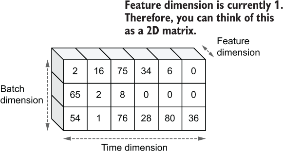
Figure 9.2 3D view of sequential data. Typically, sequential data is found with three dimensions; batch size, sequence/time, and feature.

The LSTM takes an input with the three dimensions discussed. Let’s zoom in a bit more to see how an LSTM operates on such data. To keep the discussion simple, assume a batch size of 1 or a single review. If we assume a single review r that has n words it can be written as

r = w_1,w_2,...,w_t,...,w_n, where w_t represents the ID of the word in the t^th position.

At time step t, the LSTM model starts with

• The previous output state vector h_t-1

• The previous cell state vector c_t-1

and computes

• The current cell state c_t using the current input w_t and the previous cell state c_t-1 and output state h_t-1 and

• The current output state h_t using the current input w_t and the previous state h_t-1 and the current cell state c_t

This way, the model keeps iterating over all the timesteps (in our example, it’s word IDs in the sequence) until it reaches the end. While iterating this way, the model keeps producing a cell state and an output state (figure 9.3).

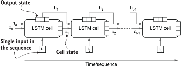
Figure 9.3 High-level longitudinal view of an LSTM cell. At a given time step t, the LSTM cell takes in two previous states (h_t-1 and c_t-1), along with the input, and produces two states (h_t and c_t).

With a good high-level understanding of the LSTM cell, let’s look at the equations that are cranking the gears of this model. The LSTM takes three inputs:

• x_t—The input at timestep t

• h_t-1—The output state at timestep t-1

• c_t-1—The cell state at timestep t-1

With that, the LSTM produces two outputs:

• (c_t)—The cell state at timestep t

• (h_t)—The output state at timestep t

To produce these outputs, the LSTM model leverages a gating mechanism. These gates determine how much information flows through them to the next stage of computations. The LSTM cell has three gates:

• An input gate (i_t)—Determines how much of the current input will affect the subsequent computations

• A forget gate (f_t)—Determines how much of the previous cell state is discarded when computing the new cell state

• An output gate (o_t)—Determines how much of the current cell state contributes to the final output

These gates are made of trainable weights. This means that when training an LSTM model on a certain task, the gating mechanism will be jointly optimized to produce the optimal flow of information required to solve that task.

You might still be wondering, “What is this gating mechanism actually achieving?” Let me illustrate that with a sentence. To solve almost all NLP tasks, capturing syntactic and semantic information as well parsing dependencies correctly in a given text input is imperative. Let’s see how an LSTM can help us to achieve that. Assume you’ve been given the sentence:

the dog ran after the green ball and it got tired and barked at a plane

In your mind, picture an LSTM model hopping from one word to another, processing them. Then assume you query the model for answers to questions at various stages of processing the sentence. Say you ask the question “Who ran?” while it’s processing the phrase “the dog ran.” The model will probably have its input gate widely open to absorb as much information as the model can, because the model starts with no prior knowledge about what language looks like. And if you think about it, the model does not really need to pay attention to its memory because the answer is one word away from the word “ran.”

Next, you ask “Who got tired?” When processing “it got tired,” the model might want to tap into its cell state instead of focusing on the input, as the only clue in this phrase is “it.” If the model is to identify the relationship between it and dog, it will need to close the input gate slightly and open the forget gate so that more information flows from the past memory (about the dog) into the current memory.

Finally, let’s say you ask “What was barked at?” by the time the model reaches the “barked at a plane” section. To produce the final output, you don’t need much information from past memory, so you might tighten the output gate to avoid too much information coming from the past memory. I hope these walkthroughs were useful in order to grok the purpose of these gates. Remember that this is just an analogy to understand the purpose of these gates. But in practice, the actual behavior can differ. It is also worth noticing that these gates are not binary; rather, the output of the gate is controlled by a sigmoidal function, meaning that it leads to a soft open/close state at a given time rather than a hard open/close state.

To complete our discussion, let’s inspect the equations that drive the computations in an LSTM cell. But you don’t have to memorize or understand these equations in detail, as it’s not a requirement to use LSTMs. But to make our discussion holistic, let’s look at them. The first computation computes the input gate:

i_t = σ(W_ihh_t-1 + W_ixx_t + b_f)

Here, W_ih and W_ix are trainable weights that produce the gate value, where b_i is the bias. The computations here closely resemble the computations of a fully connected layer. This gate results in a vector for a given input whose values are between 0 and 1. You can see its resemblance to a gate (assuming 0 means closed and 1 means open). The rest of the gates follow a similar pattern of computations. The forget gate is computed as

f_t = σ(W_fhh_t-1 + W_fxx_t + b_f)

Then the cell state is computed. Cell state is computed from a two-fold computation:

C̃_t = tanh(W_ch h_t-1 + W_cxx_t = b_c)

c_t = f_th_t-1 + i_tC̃_t

The computation is quite intuitive. It uses the forget gate to control the previous cell state, where it uses the input gate to control C̃_t computed using x_t (the current input). Finally, the output gate and the state are computed as

o_t = σ(W_ohh_t-1 + W_oxx_t + b₀)

h_t = o_ttanh(c_t)

Here, c_t is computed using the inputs controlled via the forget gate and the input gate. Therefore, in a way, o_t gets to control how much the current input, the current cell state, the previous cell state, and the previous output state contribute to the final state output of the LSTM cell. In TensorFlow and Keras, you can define an LSTM with

import tensorflow as tf
tf.keras.layers.LSTM(units=128, return_state=False, return_sequences=False)

The first argument units is a hyperparameter of the LSTM layer. Similar to how the number of units defines the output size of a fully connected layer, the units argument defines the output, state, and gate vector dimensionality. The higher this number, the more representative power the model possesses. Next, the return_state=False means only the output state will be returned when the layer is called on an input. If return_state=True, both the cell state and the output state are returned. Finally, return_sequences=False means that only the final state(s) after processing the whole sequence is returned. If return_sequences=True, all the state(s) returned during processing every element in the sequence are returned. Figure 9.4 depicts the differences in these arguments’ results.

Figure 9.4 The changes to the output of the LSTM layer resulted in changes to the return_state and return_sequences arguments.

Next, let’s define the final model.

9.4.2 Defining the final model

We will define the final model using the Sequential API. Our model will have the following layers (figure 9.5):

• A masking layer—This layer plays an important role in which input elements in the sequence will contribute to the training. We will learn more about this soon.

• A one-hot encoding layer—This layer will convert the word IDs to one-hot encoded sequences. This is an important transformation we have to perform before feeding our inputs to the model.

• An LSTM layer—The LSTM layer will return the final output state as the output.

• A Dense layer with 512 nodes (ReLU activation)—A Dense layer takes the output of the LSTM cell and produces an interim hidden output.

• A Dropout layer—Dropout is a regularization technique that randomly switches outputs during the training process. We discussed the purpose of Dropout and how it works in chapter 7.

• A final output layer with a single node (sigmoid activation)—Note that we only need a single node to represent the output. If the value of the output is 0, it’s a negative sentiment. If the value is 1, it’s a positive sentiment.

Figure 9.5 The high-level model architecture of the sentiment analyzer

Our tf.data pipeline produces a [<batch size>, <sequence length>]-shaped 2D tensor. In practice, they would both be None. In other words, it will be a [None, None]-sized tensor as we have to support variable-sized batches and variable-sized sequence lengths in our model. A dimension of size None means that the model can accept any sized tensor on that dimension. For example, with a [None, None] tensor, when actual data is retrieved, it can be a [5, 10]-, [12, 54]-, or [102, 14]-sized tensor. As the entry point to the model, we will use a reshaping layer wrapped in a lambda layer as follows:

tf.keras.layers.Lambda(lambda x: tf.expand_dims(x, axis=-1), input_shape=(None,)),

This layer takes our [None, None] input produced by the data pipeline and reshapes it to a [None, None, 1]-sized tensor. This reshaping is necessary for the next layer in line, making it a perfect opportunity to discuss the next layer. The next layer is a masking layer that serves a very special purpose. We have not seen a masking layer used in previous chapters. However, masking is commonly used in NLP problems. The need for masking arises from the padding operation we perform on the inputs during the bucketing of input sequences. In NLP data sets, you will seldom see text appearing with a fixed length. Typically, each text record has a different length. To batch these variable-sized text records together for the model, padding plays an essential role. Figure 9.6 illustrates what the data looks like after padding.

Figure 9.6 Text sequences before and after padding

But this introduces an extra burden. The values introduced by padding (typically zero) do not carry any information. Therefore, they should be ignored in any computation that happens in the model. For example, the LSTM model should halt processing and return that last state just before encountering padded values when padding is used in the input. The tf.keras.layers.Masking layer helps us to do exactly that. The input to the masking layer must be a [batch size, sequence length, feature dimension]-sized 3D tensor. This alludes to our last point about reshaping the output of our tf.data pipeline to a 3D tensor. In TensorFlow you define a mask as follows:

tf.keras.layers.Masking(mask_value=0)

The masking layer creates a special mask, and this mask is propagated to the subsequent layers in the model. Layers like the LSTM layer know what to do if a mask is passed from a layer below. More specifically, the LSTM model will output its state values just before it encountered zeros (if a mask is provided). It is also worth paying attention to the input_shape argument. The input to our model will be a two-dimensional tensor: an arbitrary-sized batch with an arbitrary-sized sequence length (due to bucketing). Therefore, we cannot specify a sequence length in the input_shape argument, so the model expects a (None, None, 1)-sized tensor as the input (the extra None is added automatically to represent the batch dimension).

With the mask defined, we will convert the word IDs to one-hot vectors using a custom layer. This is an essential step before feeding data to the LSTM. This can be achieved as follows:

class OnehotEncoder(tf.keras.layers.Layer):
    def __init__(self, depth, **kwargs):
        super(OnehotEncoder, self).__init__(**kwargs)
        self.depth = depth
 
 
    def build(self, input_shape):
        pass
 
 
    def call(self, inputs):        
        
        inputs = tf.cast(inputs, 'int32')
        
        if len(inputs.shape) == 3:
            inputs = inputs[:,:,0]
  
        return tf.one_hot(inputs, depth=self.depth)
 
            
    def compute_mask(self, inputs, mask=None):
        return mask
 
 
    def get_config(self):
        config = super().get_config().copy()
        config.update({'depth': self.depth})
        return config

Then call it with

OnehotEncoder(depth=n_vocab),

The layer is a mouthful, so let’s break it down. First you define a user-defined parameter called depth. This defines the feature dimension of the final result. Next, you have to define the call() function. The call() function takes in the inputs, casts them to 'int32', and then removes the final dimension if the input is three-dimensional. This is because the masking layer we defined has a dimension of size 1 to represent the feature dimension. This dimension is not understood by the tf.one_hot() function that we use to generate one-hot encoded vectors. Therefore, it must be removed. Finally, we return the result of the tf.one_hot() function. Remember to provide the depth parameter when using tf.one_hot(). If it is not provided, TensorFlow tries to automatically infer the value, which leads to inconsistently sized tensors between different batches. We define the compute_mask() function to make sure we propagate the mask to the next layer. The layer simply takes the mask and passes it to the next layer. Finally, we define a get_config() function to update the parameters in that layer. It is essential for config to return the correct set of parameters; otherwise, you will run into problems saving the model. We define the LSTM layer as the next layer of the model:

tf.keras.layers.LSTM(units=128, return_state=False, return_sequences=False)

We have to be extra careful here. Depending on the arguments you provide when defining this layer, you will get vastly different outputs. To define our sentiment analyzer, we only want the final output state of the model. This means we’re not interested in the cell state, nor all the output states computed during processing the sequence. Therefore, we have to set the arguments accordingly. According to our requirements, we must set return_state=False and return_sequences=False. Finally, the final state output goes to a Dense layer with 512 units and ReLU activation:

tf.keras.layers.Dense(512, activation='relu'),

The dense layer is followed by a Dropout layer that will drop 50% of the inputs of the previous Dense layer during training.

tf.keras.layers.Dropout(0.5)

Finally, the model is crowned with a Dense layer having a single unit and sigmoidal activation, which will produce the final prediction. If the produced value is less than 0.5, it is considered label 0 and 1 otherwise:

tf.keras.layers.Dense(1, activation='sigmoid')

We can define the full model as shown in the next listing.

Listing 9.5 Implementation of the full sentiment analysis model

model = tf.keras.models.Sequential([
    
    tf.keras.layers.Masking(mask_value=0.0, input_shape=(None,1)),         ❶
    OnehotEncoder(depth=n_vocab),                                          ❷
    tf.keras.layers.LSTM(128, return_state=False, return_sequences=False), ❸
    tf.keras.layers.Dense(512, activation='relu'),                         ❹
    tf.keras.layers.Dropout(0.5),                                          ❺
    tf.keras.layers.Dense(1, activation='sigmoid')                         ❻
])

❶ Create a mask to mask out zero inputs.

❷ After creating the mask, convert inputs to one-hot encoded inputs.

❸ Define an LSTM layer that returns the last state output vector (from unmasked inputs).

❹ Define a Dense layer with ReLU activation.

❺ Define a Dropout layer with 50% dropout.

❻ Define a final prediction layer with a single node and sigmoidal activation.

Next, we’re off to compiling the model. Again, we have to be careful about the loss function we will be using. So far, we have used the categorical_crossentropy loss. This loss is used for multiclass classification problems (greater than two classes). Since we’re solving a binary classification problem, we must switch to binary_crossentropy instead. Using the wrong loss function can lead to numerical instabilities and inaccurately trained models:

model.compile(loss='binary_crossentropy', optimizer='adam', metrics=['accuracy'])

Finally, let’s examine the model by printing out the summary by running model.summary():

Model: "sequential"
_________________________________________________________________
Layer (type)                 Output Shape              Param #   
=================================================================
masking (Masking)            (None, None)              0         
_________________________________________________________________
lambda (Lambda)              (None, None, 11865)       0         
_________________________________________________________________
lstm (LSTM)                  (None, 128)               6140928   
_________________________________________________________________
dense (Dense)                (None, 512)               66048     
_________________________________________________________________
dropout (Dropout)            (None, 512)               0         
_________________________________________________________________
dense_1 (Dense)              (None, 1)                 513       
=================================================================
Total params: 6,207,489
Trainable params: 6,207,489
Non-trainable params: 0
_________________________________________________________________

This is our first encounter with a sequential model. Let’s review the model summary in more detail. First, we have a masking layer that returns an output of the same size as the input (i.e., [None, None]-sized tensor). Then a one-hot encoding layer returns a tensor with a feature dimension of 11865 (which is the vocabulary size). This is because, unlike the input that had a word represented by a single integer, one-hot encoding converts it to a vector of zeros, of the size of the vocabulary, and sets the value indexed by the word ID to 1. The LSTM layer returns a [None, 128]-sized tensor. Remember that we are only getting the final state output vector, which will be a [None, 128]-sized tensor, where 128 is the number of units. This last output returned by the LSTM goes to a Dense layer with 512 nodes and ReLU activation. A dropout layer with 50% dropout follows it. Finally, a Dense layer with one node produces the final prediction: a value between 0 and 1.

In the following section, we will train the model on training data and evaluate it on validation and testing data to assess the performance of the model.

Exercise 4

Define a model that has a single LSTM layer and a single Dense layer. The LSTM model has 32 units and accepts a (None, None, 30)-sized input (this includes the batch dimension) and produces all the state outputs (instead of the final one). Next, a lambda layer should sum up the states on the time dimension to produce a (None, 32)-sized output. This output goes to the Dense layer with 10 nodes and softmax activation. You can use the tf.keras.layers.Add layer to sum up the state vectors. You will need to use the functional API to implement this.

9.5 Training and evaluating the model

We’re all set to train the model we just defined. As the first step, let’s define two pipelines: one for the training data and one for the validation data. Remember that we split our data and created three different sets: training (tr_x and tr_y), validation (v_x and v_y), and testing (ts_x and ts_y). We will use a batch size of 128:

# Using a batch size of 128
batch_size =128
 
train_ds = get_tf_pipeline(tr_x, tr_y, batch_size=batch_size, shuffle=True)
valid_ds = get_tf_pipeline(v_x, v_y, batch_size=batch_size)

Then comes a very important calculation. In fact, doing or not doing this computation can decided whether your model is going to work or not. Remember that we noticed a significant class imbalance in our data set in section 9.1. Specifically, there are more positive classes than negative classes in the data set. Here we will define a weighing factor to assign a greater weight to negative samples when computing the loss and updating weights of the model. To do that, we will define the weighing factor:

weight_neg= count(positive samples)/count(negative samples)

This will result in a > 1 factor as there are more positive samples than negative samples. We can easily compute this using the following logic:

neg_weight = (tr_y==1).sum()/(tr_y==0).sum()

This results in weight_neg~6 (i.e., approximately 6). Next, we will define the training step as follows:

model.fit(
    x=train_ds, 
    validation_data=valid_ds, 
    epochs=10, 
    class_weight={0:neg_weight, 1:1.0}
)

Here, train_ds is passed to x, but in fact contains both the inputs and targets. valid_ds, containing validation samples, is passed to validation_data argument. We will run this for 10 epochs. Finally, note that we are using the class_weight argument to tell the model that negative samples must be prioritized over positive samples (due to the under-representation in the data set). class_weight is defined as a dictionary, where the key is the class label and the value represents the weight given to the samples of that class. When passed, during the loss computations the losses resulting from negative classes will be multiplied by a factor of neg_weight, leading to more attention being given to negative samples during the optimization process. In practice, we are going to follow the same pattern as in other chapters and run the training process with three callbacks:

• A CSV logger

• A learning rate scheduler

• Early stopping

The full code looks like the following listing.

Listing 9.6 Training procedure for the sentiment analyzer

os.makedirs('eval', exist_ok=True)
 
csv_logger = tf.keras.callbacks.CSVLogger(
       os.path.join('eval','1_sentiment_analysis.log'))                       ❶
 
monitor_metric = 'val_loss'
mode = 'min'
print("Using metric={} and mode={} for EarlyStopping".format(monitor_metric, mode))
 
lr_callback = tf.keras.callbacks.ReduceLROnPlateau(
    monitor=monitor_metric, factor=0.1, patience=3, mode=mode, min_lr=1e-8    ❷
) 
 
es_callback = tf.keras.callbacks.EarlyStopping(
    monitor=monitor_metric, patience=6, mode=mode, restore_best_weights=False ❸
)
 
model.fit(
    train_ds,                                                                 ❹
    validation_data=valid_ds, 
    epochs=10, 
    class_weight={0:neg_weight, 1:1.0}, 
    callbacks=[es_callback, lr_callback, csv_logger])

❶ Log the performance metrics to a CSV file.

❷ The learning rate reduction callback

❸ The early stopping callback

❹ Train the model.

You should get similar results:

Using metric=val_loss and mode=min for EarlyStopping
Epoch 1/10
2427/2427 [==============================] - 72s 30ms/step - loss: 0.7640 - accuracy: 0.7976 - val_loss: 0.4061 - val_accuracy: 0.8193 - lr: 0.0010
 
...
 
Epoch 7/10
2427/2427 [==============================] - 73s 30ms/step - loss: 0.2752 - accuracy: 0.9393 - val_loss: 0.7474 - val_accuracy: 0.8026 - lr: 1.0000e-04
Epoch 8/10
2427/2427 [==============================] - 74s 30ms/step - loss: 0.2576 - accuracy: 0.9439 - val_loss: 0.8398 - val_accuracy: 0.8041 - lr: 1.0000e-04

It seems that by the end of the training, we have reached above 80% validation accuracy. That’s great news, because we made sure that the validation data set is a balanced data set. But we can’t be too sure. We will need to test our model on a data set that it hasn’t had the chance to see: the testing set. Before that, let’s save the model:

os.makedirs('models', exist_ok=True)
tf.keras.models.save_model(model, os.path.join('models', '1_sentiment_analysis.h5'))

We have already created the test data set and have defined the NLP pipeline to process the data, so it’s a matter of calling the get_tf_pipeline() function with the data:

test_ds = get_tf_pipeline(ts_x, ts_y, batch_size=batch_size)

It’s now as simple as calling the following one-liner to get the test performance of the model:

model.evaluate(test_ds)

The final result looks like this:

87/87 [==============================] - 2s 27ms/step - loss: 0.8678 - accuracy: 0.8038

We can now go to sleep knowing our model’s performance on unseen data is on par with the validation performance we saw during training.

In the next section, we will further enhance our model by using word vectors to represent tokens fed into the model. Word vectors help machine learning models understand language better.

Exercise 5

Assume you have three classes in your training data set: A, B and C. You have 10 records for A, 25 for B, and 50 for C. What do you think will be good weights for the three classes? Remember that the majority class should get a smaller weight.

9.6 Injecting semantics with word vectors

You have built a model that can measure sentiments with ~80% accuracy, but you want to improve further. You believe word embeddings will provide the edge required to attain a higher accuracy. Word embeddings are a way to encode words as a feature vector. Word embeddings learn feature vectors for the words in the vocabulary jointly with the model training. An embedding layer introduces a trainable matrix, where each row represents a trainable vector for a single word in the vocabulary. This is much better than one-hot encoding because one-hot encoding suffers from the curse of dimensionality, which means that as the number of words grows, so does the dimensionality of the inputs to the model.

You should feel proud about having a reasonable model that can accurately classify positive and negative sentiments; 80% accuracy is a great starting point. But let’s see what we can improve in the already good model we have.

A bottleneck that’s staring us right in the face is the one-hot encoding layer that’s in our model. One-hot encoding, despite its simplicity, is a very inefficient representation of words. It is a localized representation of words, meaning only one element (set to value 1) in the representation carries information. In other words, it’s a very sparse representation that has a very large number of elements set to zero and does not contribute with information. One-hot encoding also suffers from the curse of dimensionality. Finally, one-hot encoding completely disregards the valuable semantics present in the text. With one-hot encoding, you can’t say if a cat is more similar to a dog than it is to a volcano. Now the question is, are there better ways to represent words?

9.6.1 Word embeddings

It’s time to usher in a new era of word representations known as word embeddings. Word embeddings, sometimes called word vectors, are a very information-rich and efficient representation of words. As opposed to the localized representations like one-hot vectors, word vectors provide a distributed representation. This means that all the elements in the vector play a role in defining the word represented by the vector. In other words, word vectors have dense representations, in contrast to the sparse representation of one-hot vectors. The dimensionality of word vectors does not depend on the size of vocabulary, which allows you to save memory and computational time. Finally, but most importantly, word vectors capture the semantics or similarity of words. With word vectors, you know that a cat is more similar to a dog than to a volcano. Before understanding word vectors, you have to understand the important role played by the context around a word. Word vectors heavily rely on the context of words to generate rich representations of words. The importance of the context is subliminally captured by a famous quote by J.R. Firth, an English linguist:

You shall know a word by the company it keeps.

To expand on this a little more, the context of a word plays an important role in defining the semantics of that word. For example, take the following sentence:

Our pet Toby is a ____; he enjoys playing with a ball.

What do you think is the right word here? We see words like “pet,” “playing,” and “ball” in the context. Most likely it’s a cat or a dog. This means that only a certain type of words (i.e., a type of pet) will appear in this context. Using this property, word vectors can generate vectors that preserve the semantics of the text. In this example, word vectors will capture that cats and dogs are very similar (not biologically, of course, but in the way we interact with or perceive them). In a more technical stance, the objective of word vector algorithms is as follows: if word w_i and w_j appear in the same context, for some distance measure Dist(a,b), that measures the distance between two vectors a and b:

Dist(w_i, w_j) ~ 0

The actual word vector algorithms are out of scope for this book. A few note-worthy algorithms are Skip-gram, CBoW (Continuous Bag-of-Words), GloVe (global vectors) and ELMo (Embeddings from Language Models). You can read more details about the Skip-gram and CBoW algorithms by reading the paper “Efficient Estimation of Word Representations in Vector Space” by Tomas Mikolov et al. (https://arxiv.org/pdf/1301.3781.pdf).

The final output of a word vector algorithm is a V × d-sized embedding matrix. The i^th row of this matrix represents the word vector for the word represented by the ID i. d is typically < 300 and is selected using a hyperparameter algorithm. Figure 9.7 depicts the word embedding matrix.

Figure 9.7 An overview of how the embedding matrix is used to obtain word vectors. A lookup is performed using the input word IDs to fetch the vectors corresponding to those indices. The actual values of the vectors are learned during the model training.

We will now enhance our sentiment analyzer model with word embeddings.

9.6.2 Defining the final model with word embeddings

In general, any deep sequential model can benefit from word embeddings. As an added benefit, most of the time you don’t need to worry about the word vector algorithms themselves and can enjoy good performance by introducing a randomly initialized embedding space. Then the embeddings can be trained jointly with the other parts of the models during the specific NLP task we’re solving. Following the same pattern, let’s introduce a randomly initialized embedding space to our sentiment analyzer.

Let’s remind ourselves of the previous model we implemented. The model consisted of a masking layer, a one-hot encoder layer, and an LSTM layer followed by two Dense layers (with dropout in between):

model = tf.keras.models.Sequential([
    # Create a mask to mask out zero inputs
    tf.keras.layers.Masking(mask_value=0.0, input_shape=(None,1)),
    # After creating the mask, convert inputs to onehot encoded inputs
    OnehotEncoder(depth=n_vocab),
    # Defining an LSTM layer
    tf.keras.layers.LSTM(128, return_state=False, return_sequences=False),
    # Defining a Dense layer
    tf.keras.layers.Dense(512, activation='relu'),
    tf.keras.layers.Dropout(0.5),
    tf.keras.layers.Dense(1, activation='sigmoid')
])

The model will remain more or less the same, except for two changes:

• We will replace the one-hot encoder layer with an tf.keras.layers.Embedding layer.

• The masking functionality will be absorbed into the tf.keras.layers.Embedding layer by setting the mask_zero=True in the layer.

The tf.keras.layers.Embeddings layer introduces a large trainable matrix into the model. This matrix is a (V+1) x d-sized matrix, where V is the vocabulary size. The additional one is required as we use the special reserved ID zero. d is chosen through a hyperparameter optimization algorithm. In the following model, we will set d = 128 empirically. The line that has changed has been highlighted in bold in the listing.

Listing 9.7 Implementing the sentiment analyzer with word embeddings

model = tf.keras.models.Sequential([                                               ❶
    
    tf.keras.layers.Embedding(input_dim=n_vocab+1, output_dim=128, mask_zero=True),❷
    
    tf.keras.layers.LSTM(128, return_state=False, return_sequences=False),         ❸
    tf.keras.layers.Dense(512, activation='relu'),                                 ❹
    tf.keras.layers.Dropout(0.5),                                                  ❺
    tf.keras.layers.Dense(1, activation='sigmoid')                                 ❻
])
 
model.compile(loss='binary_crossentropy', optimizer='adam', metrics=['accuracy'])  ❼
model.summary()

❶ Create a mask to mask out zero inputs.

❷ Add an Embedding layer. It will look up word vectors for the word IDs passed in as the input.

❸ Define an LSTM layer.

❹ Define Dense layers.

❺ Define a Dropout layer.

❻ Define the final Dense layer with sigmoidal activation.

❼ Compile the model with binary cross-entropy as the loss.

UnknownError:  [_Derived_]  CUDNN_STATUS_BAD_PARAM
in tensorflow/stream_executor/cuda/cuda_dnn.cc(1496): 
➥ 'cudnnSetRNNDataDescriptor( data_desc.get(), data_type, layout, 
➥ max_seq_length, batch_size, data_size, seq_lengths_array, 
➥ (void*)&padding_fill)'
         [[{{node cond_38/then/_0/CudnnRNNV3}}]]
         [[sequential/lstm/StatefulPartitionedCall]]
         [[gradient_tape/sequential/embedding/embedding_lookup/Reshape/_42]] 
➥ [Op:__inference_train_function_8225]
 
Function call stack:
train_function -> train_function -> train_function

With that, we will train the model we defined.

9.6.3 Training and evaluating the model

Training and evaluation code are identical to the implementation we discussed earlier. Therefore, we will not reiterate the discussion. When you train the new model, you will see a result similar to the following.

When you train the model, you will reach a validation accuracy that is slightly above the previous validation accuracy we experienced:

Epoch 1/25
2427/2427 [==============================] - 30s 12ms/step - loss: 0.7552 - 
➥ accuracy: 0.7949 - val_loss: 0.3942 - val_accuracy: 0.8277 - lr: 0.0010
Epoch 2/25
 
...
 
Epoch 8/25
2427/2427 [==============================] - 29s 12ms/step - loss: 0.3059 - 
➥ accuracy: 0.9312 - val_loss: 0.6839 - val_accuracy: 0.8130 - lr: 1.0000e-04

Evaluating the model can be done by running the following:

test_ds = get_tf_pipeline(ts_x, ts_y, batch_size=128)
model.evaluate(test_ds)

It seems that adding an embedding layer leads to a slightly higher testing performance as well:

87/87 [==============================] - 0s 5ms/step - loss: 0.7214 - accuracy: 0.8111

Remember that we said we wouldn’t trust the accuracy alone. Now let’s dig in a bit deeper and see if our model is giving out sensible predictions. An easy way to do this is to check the top-k positive reviews and the top-k negative reviews in the test set and do a visual inspection. We exhausted the tf.data pipeline when we finished the evaluation. Therefore, we need to redefine the data pipeline:

test_ds = get_tf_pipeline(ts_x, ts_y, batch_size=128)

Then we will go batch by batch, and for each batch, we will store the inputs, predictions, and targets in three separate lists: test_x, test_pred, and test_y, respectively:

test_x = []
test_pred = []
test_y = []
for x, y in test_ds:
    test_x.append(x)    
    test_pred.append(model.predict(x))
    test_y.append(y)
test_x = [doc for t in test_x for doc in t.numpy().tolist()]
test_pred = tf.concat(test_pred, axis=0).numpy()
test_y = tf.concat(test_y, axis=0).numpy()

We will use argsort to get the indices of the sorted prediction array. This way, the start of the array will have the indices of the most negative reviews, whereas the end of the array will contain the most positive review indices. Let’s take the five top-most and five bottom-most reviews to visually check:

sorted_pred = np.argsort(test_pred.flatten())
min_pred = sorted_pred[:5]
max_pred = sorted_pred[-5:]
 
print("Most negative reviews
")
print("="*50)
for i in min_pred:    
    print(" ".join(tokenizer.sequences_to_texts([test_x[i]])), '
')
    
print("
Most positive reviews
")
print("="*50)
for i in max_pred:
    print(" ".join(tokenizer.sequences_to_texts([test_x[i]])), '
')

Let’s check the results:

Most negative reviews
==================================================
buy game high rating promise gameplay saw youtube story so-so graphic 
➥ mediocre control terrible could not adjust control option preference ...
 
attempt install game quad core windows 7 pc zero luck go back forth try 
➥ every suggestion rockstar support absolutely useless game ... 
 
way product 5 star 28 review write tone lot review similar play 2 song 
➥ expert drum say unless play tennis shoe fact screw not flush mean feel 
➥ every kick specifically two screw leave plus pedal completely torn 
➥ mount screw something actually go wrong pedal instal unscrew send back 
➥ ea 
 
unk interactive stranger unk unk genre develop operation flashpoint various 
➥ real-life computer sims military folk unk know come deliver good 
➥ recreation ultra deadly unk modern combat engagement arma attempt 
➥ simulate `` unk firepower '' soldier combine arm warfare set fictional 
➥ sprawl island nation conveniently mirror terrain middle eastern country 
 
not cup tea 
 
 
Most positive reviews
==================================================
find something love every final fantasy game play thus far ff13 different 
➥ really appreciate square enix 's latest trend shake gameplay new 
➥ release still hammer best look ... 
know little squad base game genre know game fun not unk fun obliterate 
➥ enemy mobile suit satisfy blow zombie head resident evil graphic 
➥ presentation solid best franchise yes ... 
 
okay hdtv monitor cause ps3 switch game movie widescreen fullscreen every 5 
➥ minute someone tell need get hd component cable look price saw brand 
➥ name sony much money basically name brand pay fancy retail packaging 
➥ generic cable get quality without fancy packaging name brand embed 
➥ cable favor save money 
 
absolutely phenomenal gaming mouse love programmable size button mouse 
➥ surprising ergonomic design ... 
 
first motorstorm come unk racing type one pioneer physic base race every 
➥ track lot branch path every branch suitable different class vehicle 
➥ take next level race much bigger apart mud also obstacles individual 
➥ vehicle class small vehicle get stuck plant unk hazard time lot physic 
➥ people complain vehicle slide 

We can confidently say that our sentiment analyzer was a success! The negative and positive reviews identified by the model seem like they’re in the correct places. We had to overcome many obstacles having to do with data quality, data preparation, and model design. Through them all, we persevered! In the next chapter, we will discuss another NLP task known as language modeling.

Exercise 6

Word vector algorithms like Skip-gram use an embedding layer directly connected to a Dense layer that has the same size as the vocabulary. If you have a vocabulary of size 500, want to produce 32 dimensional word vectors, and have a dense layer with 500 units and a softmax activation, how would you implement a model? The model accepts a (None, 500)-sized (batch dimension is None) one-hot encoded vectors of words.

Summary

• The NLTK library provides an API to perform various text preprocessing tasks, such as tokenizing to words, removing stop words, lemmatization, and so on.

• Preprocessing tasks need to be applied with care. For example, when removing stop words, the word “not” should not be removed. This is because in a sentiment analysis task, the word “not” carries very important information.

• tensorflow.keras.preprocessing.text.Tokenizer can be used to convert text to numbers. This is done by the Tokenizer first building a dictionary that maps each unique word to a unique ID. Then a given text can be converted to a sequence of IDs.

• Padding is a technique used to bring variable-length text to the same length.

• Padding works by padding all sequences in a given text corpus to a fixed length by inserting zeros (at the end or at the beginning).

• When processing variable-length sequences like text, there’s another strategy known as bucketing that is used to batch similar-length text sequences together. This helps the model keep the memory footprint small as well as to not waste computation on excessing padding.

• In TensorFlow, you can use tf.data.experimental.bucket_by_sequence_ length() to bucket text sequences.

• LSTM (long short-term memory) models have shown superior performance in solving NLP tasks.

• LSTM models work by going from one timestep to the next, while processing the input at that time step to produce an output for each timestep.

• LSTM models have a mechanism to store both long-term and short-term memory. This is achieved through a gating mechanism that controls the flow of information in the LSTM cell.

• Word embeddings are a text encoding method that is superior to one-hot encoding and that has the ability to preserve the semantics of words when generating the numerical representation of words.

Answers to exercises

Exercise 1

s = s.replace("-", ' ')
   tokens = word_tokenize(s)                                                             
pos_tags = nltk.pos_tag(tokens)
clean_text = [
        lemmatizer.lemmatize(w, pos=p[0].lower()) if p[0]=='V' else w
        for (w, p) in pos_tags
]

Exercise 2

s = “a_b_B_c_d_a_D_b_d_d”
tok = Tokenizer(num_words = 3, split=”_”, lower=True)
tok.fit_on_texts([s])
 
Most common words get the lowest word ID (starting from 1). 
➥ tok.texts_to_sequences([s]) will produce [[3,2,2,1,3,1,2,1,1]]

Exercise 3

bucket_fn = tf.data.experimental.bucket_by_sequence_length(
        lambda x: tf.cast(tf.shape(x)[0],'int32'), 
        bucket_boundaries=[10, 25, 30], 
        bucket_batch_sizes=[batch_size,batch_size,batch_size, batch_size], 
        padded_shapes=None,
        padding_values=0, 
        pad_to_bucket_boundary=True
    )

Exercise 4

inp = tf.keras.layers.Input(shape=(None, 30))
lstm_out = tf.keras.layers.LSTM(32, return_sequences=True)(inp)
sum_out = tf.keras.layers.Add(axis=1)(lstm_out)
dense_out = tf.keras.layers.Dense(10, activation=’softmax’)(sum_out)

Exercise 5

A - (25+50)/(10+25+50)
B - (10+50)/(10+25+50)
C - (10+25)/(10+25+50)

Exercise 6

tf.keras.models.Sequential(
[
    tf.keras.layers.Embedding(input_dim=500, output_dim=32, input_shape=(500,)),
    tf.keras.layers.Dense(500, activation=’softmax’)
])