
10 Natural language processing with TensorFlow: Language modeling
- Implementing an NLP data pipeline with TensorFlow
- Implementing a GRU-based language model
- Using a perplexity metric for evaluating language models
- Defining an inference model to generate new text from the trained model
- Implementing beam search to uplift the quality of generated text
In the last chapter, we discussed an important NLP task called sentiment analysis. In that chapter, you used a data set of video game reviews and trained a model to predict whether a review carried a negative or positive sentiment by analyzing the text. You learned about various preprocessing steps that you can perform to improve the quality of the text, such as removing stop words and lemmatizing (i.e., converting words to a base form; e.g., plural to singular). You used a special type of model known as long short-term memory (LSTM). LSTM models can process sequences such as sentences and learn the relationships and dependencies in them to produce an outcome. LSTM models do this by maintaining a state (or memory) containing information about the past, as it processes a sequence one element at a time. The LSTM model can use the memory of past inputs it has seen along with the current input to produce an output at any given time.
In this chapter, we will discuss a new task known as language modeling. Language modeling has been at the heart of NLP. Language modeling refers to the task of predicting the next word given a sequence of previous words. For example, given the sentence, “I went swimming in the ____,” the model would predict the word “pool.” Ground-shattering models like BERT (bidirectional encoder representation from Transformers, which is a type of Transformer-based model) are trained using language modeling tasks. This is a prime example of how language modelling can help to actualize innovative models that go on to be used in a plethora of areas and use cases.
In my opinion, language modeling is an underdog in the world of NLP. It is not appreciated enough, mostly due to the limited use cases the task itself helps to realize. However, language modeling can provision the much-needed linguistic knowledge (e.g., semantics, grammar, dependency parsing, etc.) to solve other downstream use cases (e.g., information retrieval, question answering, machine translation, etc.). Therefore, as an NLP practitioner, you must understand the language modeling task.
In this chapter, you will build a language model. You will learn about the various preprocessing steps involved, such as using n-grams instead of full words as features for the model to reduce the size of the vocabulary. You can convert any text to n-grams by splitting it every n characters (e.g., if you use bi-grams, aabbbccd becomes aa, bb, bc, and cd). You will define a tf.data pipeline that will do most of this preprocessing for us. Next, you will use a close relative of the LSTM model known as gated recurrent unit (GRU) to do the language modeling task. GRU is much simpler than the LSTM model, making it faster to train while maintaining similar performance to the LSTM model. We will use a special metric called perplexity to measure how good our model is. Perplexity measures how surprised the model was to see the next word in the corpus given the previous words. You will learn more about this metric later in the chapter. Finally, you will learn about a technique known as beam search, which can uplift the quality of the text generated by the model by a significant margin.
10.1 Processing the data
You’ve been closely following a new generation of deep learning models that have emerged, known as Transformers. These models have been trained using language modeling. It is a technique that can be used to train NLP models to generate stories/ Python code/movie scripts, depending on the training data used. The idea is that when a sequence of n words, predict the n + 1 word. The training data can easily be generated from a corpus of text by taking a sequence of text as the input and shifting it right by 1 to generate the targets. This can be done at a character level, word level, or n-gram level. We will use two-grams for the language modeling task. We will use a children’s story data set from Facebook known as bAbI (https://research.fb.com/downloads/babi/). You will create a TensorFlow data pipeline that performs these transformations to generate inputs and targets from text.
10.1.1 What is language modeling?
We have briefly discussed the task of language modeling. In a nutshell, language modeling, for the text w1, w2, ..., wn-1, wn, where wi is the ith word in the text, computes the probability of wn given w1, w2, ..., wn-1. In mathematical notation
In other words, it predicts wn given w1, w2, ..., wn-1. When training the model, we train it to maximize this probability; in other words
argmaxW P(w n|w1, w2, ..., wn-1)
where the probability is computed using a model that has the trainable weights/ parameters W. This computation becomes computationally infeasible for large texts, as we need to look at it from the current word all the way to the very first word. To make this computationally realizable, let’s use the Markov property, which states that you can approximate this sequence with limited history; in other words
P(w n|w1, w2, ..., wn-1) ≈ P(w n|wk, wk+1, ..., wn-1) for some k
As you can imagine, the smaller the k, the better the approximation is.
10.1.2 Downloading and playing with data
As the very first step, let’s download the data set using the code in the following listing.
Listing 10.1 Downloading the Amazon review data set
import os
import requests
import tarfile

import shutil
# Retrieve the data
if not os.path.exists(os.path.join('data', 'lm','CBTest.tgz')):      ❶
    url = "http:/ /www.thespermwhale.com/jaseweston/babi/CBTest.tgz"
    # Get the file from web
    r = requests.get(url)

    if not os.path.exists(os.path.join('data','lm')):
        os.mkdir(os.path.join('data','lm'))

    # Write to a file
    with open(os.path.join('data', 'lm', 'CBTest.tgz'), 'wb') as f:  ❷
        f.write(r.content)

else:
    print("The tar file already exists.")

if not os.path.exists(os.path.join('data', 'lm', 'CBTest')):         ❸
    # Write to a file
    tarf = tarfile.open(os.path.join("data","lm","CBTest.tgz"))
    tarf.extractall(os.path.join("data","lm"))
else:
    print("The extracted data already exists")
❶ If the tgz file containing data has not been downloaded, download the data.
❷ Write the downloaded data to the disk.
❸ If the tgz file is available but has not been extracted, extract it to the given directory.
Listing 10.1 will download the data to a local folder if it doesn’t already exist and extract the content. If you look in the data folder (specifically, data/lm/CBTest/data), you will see that it has three text files: cbt_train.txt, cbt_valid.txt, and cbt_test.txt. Each file contains a set of stories. We are going to read these files into memory. We will define a simple function to read these files into memory in the next listing.
Listing 10.2 Reading the stories in Python
def read_data(path):
    stories = []                                           ❶

    with open(path, 'r') as f:
        s = []                                             ❷
        for row in f:

            if row.startswith("_BOOK_TITLE_"):             ❸
                if len(s)>0:
                    stories.append(' '.join(s).lower())    ❹
                s = []                                     ❺

            s.append(row)                                  ❻


    if len(s)>0:
        stories.append(' '.join(s).lower())                ❼

    return stories
❶ Define a list to hold all the stories.
❷ Define a list to hold a story.
❸ Whenever, we encounter a line that starts with _BOOK_TITLE, it’s a new story.
❹ If we saw the beginning of a new story, add the already existing story to the list stories.
❺ Reset the list containing the current story.
❻ Append the current row of text to the list s.
❼ Handle the edge case of the last story remaining in s once the loop is over.
This code opens a given file and reads it row by row. We do have some additional logic to break the text into individual stories. As said earlier, each file contains multiple stories. And we want to create a list of strings at the end, where each string is a single story. The previous function does that. Next, we can read the text files and store them in variables like this:
stories = read_data(os.path.join('data','lm','CBTest','data','cbt_train.txt'))
val_stories = read_data(os.path.join('data','lm','CBTest','data','cbt_valid.txt'))
test_stories = read_data(os.path.join('data','lm','CBTest','data','cbt_test.txt'))
Here, stories will contain the training data, val_stories will contain the validation data, and finally, test_stories will contain test data. Let’s quickly look at some high-level information about the data set:
print("Collected {} stories (train)".format(len(stories)))
print("Collected {} stories (valid)".format(len(val_stories)))
print("Collected {} stories (test)".format(len(test_stories)))
print(stories[0][:100])
print('
', stories[10][:100])
This code checks how many stories are in each data set and prints the first 100 characters in the 11th story in the training set:
Collected 98 stories (train)
Collected 5 stories (valid)
Collected 5 stories (test)

chapter i. -lcb- chapter heading picture : p1.jpg -rcb- how the fairies
➥ were not invited to court .


 a tale of the tontlawald long , long ago there stood in the midst of a
➥ country covered with lakes a
Out of curiosity, let’s also analyze the vocabulary size we have to work with. To analyze the vocabulary size, we will first convert our list of strings to a list of lists of strings, where each string is a single word. Then we can leverage the built-in Counter object to get the word frequency of the text corpus. After that, we will create a pandas Series object with the frequencies as the values and words as indices and see how many words occur more than 10 times:
from collections import Counter
# Create a large list which contains all the words in all the reviews
data_list = [w for doc in stories for w in doc.split(' ')]

# Create a Counter object from that list
# Counter returns a dictionary, where key is a word and the value is the frequency
cnt = Counter(data_list)

# Convert the result to a pd.Series
freq_df = pd.Series(
    list(cnt.values()), index=list(cnt.keys())
).sort_values(ascending=False)

# Count of words >= n frequent
n=10
print("Vocabulary size (>={} frequent): {}".format(n, (freq_df>=n).sum())), 348650
the 242890
.
192549
and 179205
to 120821
a 101990
of 96748
i 79780
he 78129
was 66593
dtype: int64
Vocabulary size (>=10 frequent): 14473Nearly 15,000 words; that’s quite a vocabulary—and that’s just the words that appear more than 10 times. In the previous chapter, we dealt with a vocabulary of approximately 11,000 words. So why should we be worried about the extra 4,000? Because more words mean more features for the model, and that means a larger number of parameters and more chances of overfitting. The short answer is it really depends on your use case.
For example, in the sentiment analysis model we had in the last chapter, the final prediction layer was a single-node fully connected layer, regardless of the vocabulary size. However, in language modeling, the final prediction layer’s dimensionality depends on the vocabulary size, as the final goal is to predict the next word. This is done through a softmax layer that represents the probabilistic likelihood of the next word over the whole vocabulary, given a sequence of words. Not only the memory requirement, but also the computational time, increase as the softmax layer grows. Therefore, it is worthwhile investigating other techniques to reduce the vocabulary size.


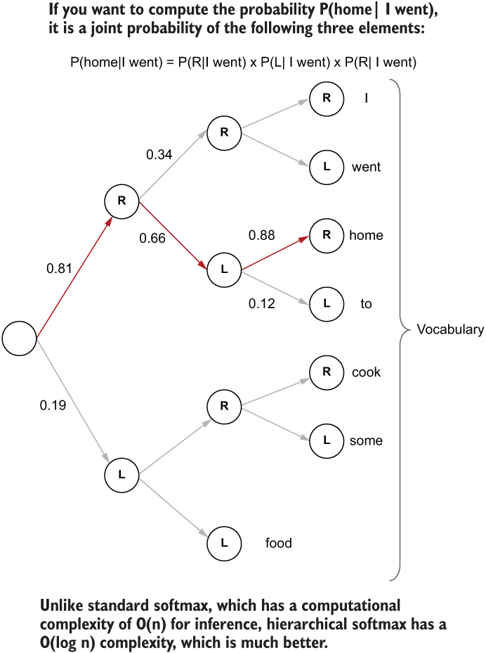
Hierarchical softmax representation of the final layer. The dark path represents the path the model must follow to compute the probability of P(home| I went).
Next, we will see how we can deal with language in the case of a large vocabulary.
10.1.3 Too large vocabulary? N-grams to the rescue
Here, we start the first step of defining various text preprocessors and the data pipeline. We suspect that going forward with a large vocabulary size can have adverse repercussions on our modeling journey. Let’s find some ways to reduce the vocabulary size. Given that children’s stories use a relatively simple language style, we can represent text as n-grams (at the cost of the expressivity of our model). N-grams are an approach where a word is decomposed to finer sub-words of fixed length. For example, the bigrams (or two-grams) of the sentence
I went to the bookshop
"I ", " w", "we", "en", "nt", "t ", " t", "to", "o ", "th", "he", "e ", " b", "bo", "oo", "ok", "ks", "sh", "ho", "op"
"I w", " we", "wen", "ent", "nt ", "t t", " to", "to ", "o t", " th", "the", "he ", "e b", " bo", "boo", "ook", "oks", "ksh", "sho", "hop"
The unigrams (or one-grams) would simply be the individual characters. In other words, we are moving a window of fixed length (with a stride of 1), while reading the characters within that window at a time. You could also generate n-grams without overlaps by moving the window at a stride equal to the length of the window. For example, bigrams without overlapping would be
"I ", "we", "nt", " t", "o ", "th", "e ", "bo", "ok", "sh", "op"
Which one to use depends on your use case. For the language modeling task, it makes sense to use the non-overlapping approach. This is because by joining the n-grams that we generated, we can easily generate readable text. For certain use cases, the non-overlapping approach can be disadvantageous as it leads to a coarser representation of text because it doesn’t capture all the different n-grams that appear in text.
By using bigrams instead of words to develop your vocabulary, you can cut down the size of the vocabulary by a significant factor. There are many other advantages that come with the n-gram approach, as we will see soon. We will write a function to generate n-grams given a text string:
def get_ngrams(text, n):
    return [text[i:i+n] for i in range(0,len(text),n)]
All we do here is go from the beginning to the end of the text with a stride equal to n and read the sequence of characters from position i to i+n. We can test how this performs on sample text:
test_string = "I like chocolates"
print("Original: {}".format(test_string))
for i in list(range(3)):
    print("	{}-grams: {}".format(i+1, get_ngrams(test_string, i+1)))
This will print the following output:
Original: I like chocolates
    1-grams: ['I', ' ', 'l', 'i', 'k', 'e', ' ', 'c', 'h', 'o', 'c',
➥ 'o', 'l', 'a', 't', 'e', 's']
    2-grams: ['I ', 'li', 'ke', ' c', 'ho', 'co', 'la', 'te', 's']
    3-grams: ['I l', 'ike', ' ch', 'oco', 'lat', 'es']
Let’s now repeat the process for analyzing the vocabulary size, but with n-grams instead of words:
from itertools import chain
from collections import Counter

# Create a counter with the bi-grams
ngrams = 2

text = chain(*[get_ngrams(s, ngrams) for s in stories])
cnt = Counter(text)

# Create a pandas series with the counter results
freq_df = pd.Series(list(cnt.values()), index=list(cnt.keys())).sort_values(ascending=False)
Now, if we check the number of words that appear at least 10 times in the text
n_vocab = (freq_df>=10).sum()
print("Size of vocabulary: {}".format(n_vocab))Size of vocabulary: 735
Wow! Compared to the 15,000 words we had, 735 is much smaller and more manageable.
10.1.4 Tokenizing text
We will tokenize the text now (i.e., split a string into a list of smaller tokens—words). By the end of this section, you will have defined and fitted a tokenizer on the bigrams generated for your text. First, let’s import the Tokenizer from TensorFlow:
from tensorflow.keras.preprocessing.text import Tokenizer
We don’t have to do any preprocessing and want to convert text to word IDs as it is. We will define the num_words argument to limit the vocabulary size as well as an oov_token that will be used to replace all the n-grams that appear less than 10 times in the training corpus:
tokenizer = Tokenizer(num_words=n_vocab, oov_token='unk', lower=False)
Let’s generate n-grams from the stories in training data. train_ngram_stories will be a list of lists of strings, where the inner list represents a list of bigrams for a single story and the outer list represents all the stories in the training data set:
train_ngram_stories = [get_ngrams(s,ngrams) for s in stories]
We will fit the Tokenizer on the two-grams of the training stories:
tokenizer.fit_on_texts(train_ngram_stories)
Now convert all training, validation, and testing stories to sequences of IDs, using the already fitted Tokenizer trained using two-grams from the training data:
train_data_seq = tokenizer.texts_to_sequences(train_ngram_stories)

val_ngram_stories = [get_ngrams(s,ngrams) for s in val_stories]
val_data_seq = tokenizer.texts_to_sequences(val_ngram_stories)

test_ngram_stories = [get_ngrams(s,ngrams) for s in test_stories]
test_data_seq = tokenizer.texts_to_sequences(test_ngram_stories)
Let’s analyze how the data looks after converting to word IDs by printing some test data. Specifically, we’ll print the first three story strings (test_stories), n-gram strings (test_ngram_stories), and word ID sequences (test_data_seq):
Original: the yellow fairy book the cat and the mouse in par
n-grams: ['th', 'e ', 'ye', 'll', 'ow', ' f', 'ai', 'ry', ' b', 'oo', 'k ',
➥ 'th', 'e ', 'ca', 't ', 'an', 'd ', 'th', 'e ', 'mo', 'us', 'e ', 'in',
➥ ' p', 'ar']
Word ID sequence: [6, 2, 215, 54, 84, 35, 95, 146, 26, 97, 123, 6, 2, 128,
➥ 8, 15, 5, 6, 2, 147, 114, 2, 17, 65, 52]


Original: chapter i. down the rabbit-hole alice was beginnin
n-grams: ['ch', 'ap', 'te', 'r ', 'i.', ' d', 'ow', 'n ', 'th', 'e ', 'ra',
➥ 'bb', 'it', '-h', 'ol', 'e ', 'al', 'ic', 'e ', 'wa', 's ', 'be', 'gi',
➥ 'nn', 'in']
Word ID sequence: [93, 207, 57, 19, 545, 47, 84, 18, 6, 2, 126, 344,
➥ 38, 400, 136, 2, 70, 142, 2, 66, 9, 71, 218, 251, 17]


Original: a patent medicine testimonial `` you might as well
n-grams: ['a ', 'pa', 'te', 'nt', ' m', 'ed', 'ic', 'in', 'e ', 'te', 'st',
➥ 'im', 'on', 'ia', 'l ', '``', ' y', 'ou', ' m', 'ig', 'ht', ' a', 's ',
➥ 'we', 'll']
Word ID sequence: [60, 179, 57, 78, 33, 31, 142, 17, 2, 57, 50, 125, 43,
➥ 266, 56, 122, 92, 29, 33, 152, 149, 7, 9, 103, 54]
10.1.5 Defining a tf.data pipeline
Now the preprocessing has happened, and we have text converted to word ID sequences. We can define the tf.data pipeline that will deliver the final processed data ready to be consumed by the model. The main steps involved in the process are illustrated in figure 10.1.
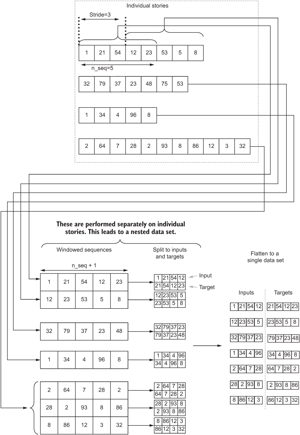
Figure 10.1 The high-level steps of the data pipeline we will be developing. First the individual stories are broken down to fixed-length sequences (or windows). Then, from the windowed sequences, inputs and targets are generated.
As we did before, let’s define the word ID corpus as a tf.RaggedTensor object, as the sentences in the corpus have variable sequence lengths:
text_ds = tf.data.Dataset.from_tensor_slices(tf.ragged.constant(data_seq))
Remember that a ragged tensor is a tensor that has variable-sized dimensions. Then we will shuffle the data so that stories come at a random order if shuffle is set to True (e.g., training time):
if shuffle:
    text_ds = text_ds.shuffle(buffer_size=len(data_seq)//2)
Now comes the tricky part. In this section, we will see how to generate fixed-sized windowed sequences from an arbitrarily long text. We will do that through a series of steps. This section can be slightly complex compared to the rest of the pipeline. This is because there will be interim steps that result in data sets nested up to three levels. Let’s try to go through this in as much detail as possible.
First, let’s make it clear what we need to achieve. The first steps we need to perform are to do the following for each individual story S:
-
Create a tf.data.Dataset() object containing the word IDs of the story S as its items.
-
Call the tf.data.Dataset.window() function to window word IDs with a n_seq+1-sized window and a predefined shift. The window() function returns a WindowDataset object for each story S.
After this, you will have a three-level nested data structure having the specification
tf.data.Dataset(              # <- From the original dataset
  tf.data.Dataset(    # <- From inner dataset containing word IDs of story S only
    tf.data.WindowDataset(...)  # <- Dataset returned by the window() function
  )
)
We will need to flatten this data set and untangle the nesting in our data set to end up with a flat tf.data.Dataset. You can remove these inner nestings using the tf.data.Dataset.flat_map() function. We will soon see how to use the flat_ map() function. To be specific, we have to use two flat_map calls to remove two levels of nesting so that we end up with only the flat original data set containing simple tensors as elements. In TensorFlow, this process can be achieved using the following line of code:
    text_ds = text_ds.flat_map(
        lambda x: tf.data.Dataset.from_tensor_slices(
            x
        ).window(
            n_seq+1,shift=shift
        ).flat_map(
            lambda window: window.batch(n_seq+1, drop_remainder=True)
        )
    )
    )
This is what we are doing here: first, we create a tf.data.Dataset object from a single story (x) and then call the tf.data.Dataset.window() function on that to create the windowed sequences. This windowed sequence contains windows, where each window is a sequence with n_seq+1 consecutive elements in the story x.
Then we call the tf.data.Dataset.flat_map() function, where, for each window element, we get all the individual IDs as a single batch. In other words, a single window element produces a single batch with all the elements in that window. Make sure you use drop_remainder=True; otherwise, the data set will return smaller subwindows within that window that contain fewer elements. Using tf.data.Dataset.flat_map() instead of map makes sure that the inner-most nesting will be removed. This whole thing is called with a tf.data.Dataset.flat_map() call, which gets rid of the next level of nesting immediately following the innermost nesting we removed. It is quite a complex process for a single liner. I suggest you go through it again if you have not fully understood the process.
You might notice that we are defining the window size as n_seq+1 and not n_seq. The reason for this will become evident later, but using n_seq+1 makes our life so much easier when we have to generate inputs and targets from the windowed sequences.
The hardest part of our data pipeline is done. By now, you have a flat data set, and each item is n_seq+1 consecutive word IDs belonging to a single story. Next, we will perform a window-level shuffle on the data. This is different from the first shuffle we did as that was on the story level (i.e., not the window level):
    # Shuffle the data (shuffle the order of n_seq+1 long sequences)
    if shuffle:
        text_ds = text_ds.shuffle(buffer_size=10*batch_size)
We’re then going to batch the data so that we will get a batch of windows every time we iterate the data set:
    # Batch the data
    text_ds = text_ds.batch(batch_size)
Finally, the reason we chose the sequence length as n_seq+1 will become clearer. Now we will split the sequences into two versions, where one sequence will be the other shifted to the right by 1. In other words, the targets to this model will be inputs shifted to the right by 1. For example, if the sequence is [0,1,2,3,4], then the two resulting sequences will be [0,1,2,3] and [1,2,3,4]. Furthermore, we will use prefetching to speed up the data ingestion:
    # Split each sequence to an input and a target
    text_ds = tf.data.Dataset.zip(
        text_ds.map(lambda x: (x[:,:-1], x[:, 1:]))
    ).prefetch(buffer_size=tf.data.experimental.AUTOTUNE)
Finally, the full code can be encapsulated in a function as in the next listing.
Listing 10.3 The tf.data pipeline from free text sequences
def get_tf_pipeline(data_seq, n_seq, batch_size=64, shift=1, shuffle=True):
    """ Define a tf.data pipeline that takes a set of sequences of text and
    convert them to fixed length sequences for the model """

    text_ds = tf.data.Dataset.from_tensor_slices(tf.ragged.constant(data_seq))❶

    if shuffle:
        text_ds = text_ds.shuffle(buffer_size=len(data_seq)//2)               ❷

    text_ds = text_ds.flat_map(                                               ❸
        lambda x: tf.data.Dataset.from_tensor_slices(
            x
        ).window(
            n_seq+1, shift=shift
        ).flat_map(
            lambda window: window.batch(n_seq+1, drop_remainder=True)
        )
    )

    if shuffle:
        text_ds = text_ds.shuffle(buffer_size=10*batch_size)                  ❹

    text_ds = text_ds.batch(batch_size)                                       ❺

    text_ds = tf.data.Dataset.zip(
        text_ds.map(lambda x: (x[:,:-1], x[:, 1:]))
    ).prefetch(buffer_size=tf.data.experimental.AUTOTUNE)                     ❻

    return text_ds
❶ Define a tf.dataset from a ragged tensor created from data_seq.
❷ If shuffle is set, shuffle the data (shuffle story order).
❸ Here we create windows from longer sequences, given a window size and a shift, and then use a series of flat_map operations to remove the nesting that’s created in the process.
❹ Shuffle the data (shuffle the order of the windows generated).
❻ Split each sequence into an input and a target and enable pre-fetching.
All this hard work wouldn’t mean as much as it should unless we looked at the generated data
ds = get_tf_pipeline(train_data_seq, 5, batch_size=6)

for a in ds.take(1):
print(a)(
<tf.Tensor: shape=(6, 5), dtype=int32, numpy=
array([[161, 12, 69, 396, 17],
[ 2, 72, 77, 84, 24],
[ 87, 6, 2, 72, 77],
[276, 484, 57, 5, 15],
[ 75, 150, 3, 4, 11],
[ 11, 73, 211, 35, 141]])>,
<tf.Tensor: shape=(6, 5), dtype=int32, numpy=
array([[ 12, 69, 396, 17, 44],
[ 72, 77, 84, 24, 51],
[ 6, 2, 72, 77, 84],
[484, 57, 5, 15, 67],
[150, 3, 4, 11, 73],
[ 73, 211, 35, 141, 98]])>
)Great, you can see that we get a tuple of tensors as a single batch: inputs and targets. Moreover, you can validate the correctness of the results, as we can clearly see that the targets are the input shifted to the right by 1. One last thing: we will save the same hyperparameters to the disk. Particularly
print("n_grams uses n={}".format(ngrams))
print("Vocabulary size: {}".format(n_vocab))

n_seq=100
print("Sequence length for model: {}".format(n_seq))

with open(os.path.join('models', 'text_hyperparams.pkl'), 'wb') as f:
    pickle.dump({'n_vocab': n_vocab, 'ngrams':ngrams, 'n_seq': n_seq}, f)
Here, we are defining the sequence length n_seq=100; this is the number of bigrams we will have in a single input/label sequence.
In this section, we learned about the data used for language modeling and defined a capable tf.data pipeline that can convert sequences of text into input label sequences that can be used to train the model directly. Next, we will define a machine learning model to generate text with.
You are given a sequence x that has values [1,2,3,4,5,6,7,8,9,0]. You have been asked to write a tf.data pipeline that generates an input and target tuple, and the target is the input shifted two elements to the right (i.e., the target of the input 1 is 3). You have to do this so that a single input/target has three elements and no overlap between the consecutive input sequences. For the previous sequence it should generate [([1,2,3], [3,4,5]), ([6,7,8], [8,9,0])].
10.2 GRUs in Wonderland: Generating text with deep learning
Now we’re on to the rewarding part: implementing a cool machine learning model. In the last chapter, we talked about deep sequential models. Given the sequential nature of the data, you probably have guessed that we’re going to use one of the deep sequential models like LSTMs. In this chapter, we will use a slightly different model called gated recurrent units (GRUs). The principles that drive the computations in the model remain the same as LSTMs. To maintain the clarity of our discussion, it’s worthwhile to remind ourselves how LSTM models work.
LSTMs are a family of deep neural networks that are specifically designed to process sequential data. They process a sequence of inputs, one input at a time. An LSTM cell goes from one input to the next while producing outputs (or states) at each time step (figure 10.2). Additionally, to produce the outputs of a given time step, LSTMs uses previous outputs (or states) it produced. This property is very important for LSTMs and gives them the ability to memorize things over time.

Figure 10.2 Overview of the LSTM model and how it processes a sequence of inputs spread over time
Let’s summarize what we learned about LSTMs in the previous chapter, as that will help us to compare LSTMs and GRUs. An LSTM has two states known as the cell state and the output state. The cell state is responsible for maintaining long-term memory, whereas the output state can be thought of as the short-term memory. The outputs and interim results within an LSTM cell are controlled by three gates:
-
Input gate—Controls the amount of the current input that will contribute to the final output at a given time step
-
Forget gate—Controls how much of the previous cell state affects the current cell state computation
-
Output gate—Controls how much the current cell state contributes to the final output produced by the LSTM model
The GRU model was introduced in the paper “Learning Phrase Representations using RNN Encoder-Decoder for Statistical Machine Translation” by Cho et al. (https://arxiv.org/pdf/1406.1078v3.pdf). The GRU model can be considered a simplification of the LSTM model while preserving on-par performance. The GRU cell has two gates:
-
Update gate (zt)—Controls how much of the previous hidden state is carried to the current hidden state
-
Reset gate (rt)—Controls how much of the hidden state is reset with the new input
Unlike the LSTM cell, a GRU cell has only one state vector. In summary, there are two major changes in a GRU compared to an LSTM model:
-
Both the input gate and forget gate are combined into a single gate called the update gate (zt). The input gate is computed as (1-zt), whereas the forget gate stays zt.
-
There’s only one state (ht) in contrast to the two states found in an LSMT cell (i.e., cell state and the output state).
Figure 10.3 depicts the various components of the GRU cell. Here is the full list of equations that make a GRU spin:
h̃t = tanh(Wh(rht-1) + Wxxt + b)

Figure 10.3 Overview of the computations transpiring in a GRU cell
This discussion was immensely helpful to not only understand the GRU model but also to learn how it’s different from an LSTM cell. You can define a GRU cell in TensorFlow as follows:
tf.keras.layers.GRU(units=1024, return_state=False, return_sequences=True)
The parameter units, return_state and return_sequences, have the same meaning as they do in the context of an LSTM cell. However, note that the GRU cell has only one state; therefore, if return_state=true, the same state is duplicated to mimic the output state and the cell state of the LSTM layer. Figure 10.4 shows what these parameters do for a GRU layer.
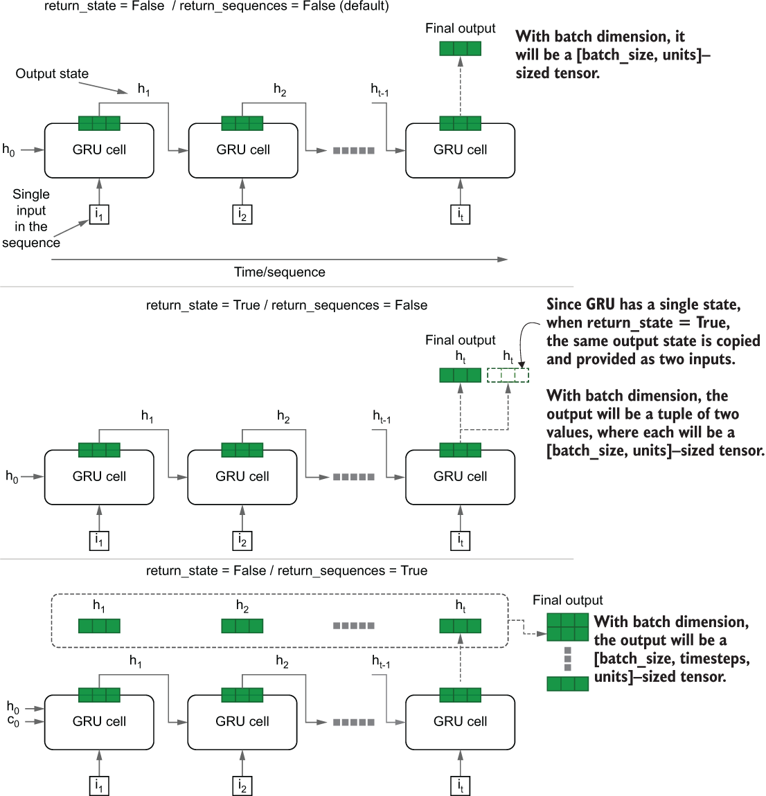
Figure 10.4 Changes in results depending on the return_state and return_sequences arguments of the GRU cell
We now know everything we need to define the final model (listing 10.4). Our final model will consist of
-
A GRU layer (1,024 units) that returns all the final state vectors as a tensor that has shape [batch size, sequence length, number of units]
Listing 10.4 Implementing the language model
model = tf.keras.models.Sequential([
    tf.keras.layers.Embedding(
        input_dim=n_vocab+1, output_dim=512,input_shape=(None,)           ❶
    ),

    tf.keras.layers.GRU(1024, return_state=False, return_sequences=True), ❷

    tf.keras.layers.Dense(512, activation='relu'),                        ❸

    tf.keras.layers.Dense(n_vocab, name='final_out'),                     ❹
    tf.keras.layers.Activation(activation='softmax')                      ❹
])
❶ Define an embedding layer to learn word vectors of the bigrams.
❹ Define a final Dense layer and softmax activation.
You will notice that the Dense layer after the GRU receives a three-dimensional tensor (as opposed to the typical two-dimensional tensor passed to Dense layers). Dense layers are smart enough to work with both two-dimensional and three-dimensional inputs. If the input is three-dimensional (like in our case), then a Dense layer that accepts a [batch size, number of units] tensor is passed through all the steps in the sequence to generate the Dense layer’s output. Also note how we are separating the softmax activation from the Dense layer. This is actually an equivalent of
.Dense(n_vocab, activation=’softmax’, name=’final_out’)
We will not prolong the conversation by reiterating what’s shown in listing 10.4, as it is self-explanatory.
You have been given the model as follows and have been asked to add another GRU layer with 512 units that returns all the state outputs, on top of the existing GRU layer. What changes would you make to the following code?
model = tf.keras.models.Sequential([
    tf.keras.layers.Embedding(
        input_dim=n_vocab+1, output_dim=512,input_shape=(None,)
    ),
    tf.keras.layers.GRU(1024, return_state=False, return_sequences=True),
    tf.keras.layers.Dense(n_vocab, activation=’softmax’, name='final_out'), ])
In this section, we learned about gated recurrent units (GRUs) and how they compare to LSTMs. Finally, we defined a language model that can be trained on the data we downloaded and processed earlier. In the next section, we are going to learn about evaluation metrics for assessing the quality of generated text.
10.3 Measuring the quality of the generated text
Performance monitoring has been an integral part of our modeling journey in every chapter. It is no different here. Performance monitoring is an important aspect of our language model, and we need to find metrics that are suited for language models. Naturally, given that this is a classification task, you might be thinking, “Wouldn’t accuracy be a good choice for a metric?” Well, not quite in this task.
For example, if the language model is given the sentence “I like my pet dog,” then when asked to predict the missing word given “I like my pet ____,” the model might predict “cat,” and the accuracy would be zero. But that’s not correct; “cat” makes as much sense as “dog” in this example. Is there a better solution here?
Enter perplexity! Intuitively, perplexity measures how “surprised” the model was to see a target given the previous word sequence. Before understanding perplexity, you need to understand what “entropy” means.
Entropy is a term coined by the famous Claude Shannon, who is considered the father of information theory. Entropy measures the surprise/uncertainty/randomness of an event. The event can have some outcome generated by an underlying probability distribution over all the possible outcomes. For example, if you consider tossing a coin (with a probability p of landing on heads) an event, if p = 0.5, you will have the maximum entropy, as that is the most uncertain scenario for a coin toss. If p = 1 or p = 0, then you have the minimum entropy, as you know what the outcome is before tossing the coin.
The original interpretation of entropy is the expected value of the number of bits required to send a signal or a message informing of an event. A bit is a unit of memory, which can be 1 or 0. For example, you are the commander of an army that’s at war with countries A and B. Now you have four possibilities: A and B both surrender, A wins and B loses, A loses and B wins, and both A and B win. If all these events are equally likely to happen, you need two bits to send a message, where each bit represents whether that country won. Entropy of a random variable X is quantified by the equation

where x is an outcome of X. Believe it or not, we have been using this equation without knowing it every time we used the categorical cross-entropy loss. The crux of the categorical cross entropy is this equation. Coming back to the perplexity measure, perplexity is simply
Since perplexity is a function of entropy, it measures how surprised/uncertain the model was to see the target word, given the sequence of previous words. Perplexity can also be thought of as the number of all possible combinations of a given signal. For example, assume you are sending a message with two bits, where all the events are equally likely; then the entropy = 2, which means perplexity = 2^2 = 4. In other words, there are four combinations two bits can be in: 00, 01, 10, and 11.
In more of a modeling perspective, you can think of perplexity as the number of different targets that the model thinks fit the blank as the next word, given a sequence of previous words. The smaller this number, the better, as that means the model is trying to find a word from a smaller subset, indicating signs of language understanding.
To implement perplexity, we will define a custom metric. The computation is very simple. We compute the categorical cross entropy and then exponentiate it to get the perplexity. The categorical cross entropy is simply an extension of the entropy to measure entropy in classification problems with more than two classes. For an input example (xi,yi), it is typically defined as
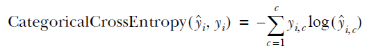
where yi denotes the one-hot encoded vector representing the true class the example belongs to and ŷi is the predicted class probability vector of C elements, with ŷi,c denoting the probability of the example belonging to class c. Note that in practice, an exponential (natural) base is used instead of base, 2 as the computations are faster. The following listing delineates the process.
Listing 10.5 Implementation of the perplexity metric
import tensorflow.keras.backend as K

class PerplexityMetric(tf.keras.metrics.Mean):

    def __init__(self, name='perplexity', **kwargs):
      super().__init__(name=name, **kwargs)
      self.cross_entropy = tf.keras.losses.SparseCategoricalCrossentropy(
         from_logits=False, reduction='none'
       )

    def _calculate_perplexity(self, real, pred):   ❶

      loss_ = self.cross_entropy(real, pred)       ❷

      mean_loss = K.mean(loss_, axis=-1)           ❸
      perplexity = K.exp(mean_loss)                ❹

      return perplexity

    def update_state(self, y_true, y_pred, sample_weight=None):
      perplexity = self._calculate_perplexity(y_true, y_pred)
      super().update_state(perplexity)
❶ Define a function to compute perplexity given real and predicted targets.
❷ Compute the categorical cross-entropy loss.
❸ Compute the mean of the loss.
❹ Compute the exponential of the mean loss (perplexity).
What we’re doing is very simple. First, we subclass the tf.keras.metrics.Mean class. The tf.keras.metrics.Mean class will keep track of the mean value of any outputted metric passed into its update_state() function. In other words, when we subclass the tf.keras.metrics.Mean class, we don’t specifically need to manually compute the mean of the accumulated perplexity metric as the training continues. It will be automatically done by that parent class. We will define the loss function we will use in the self.cross_entropy variable. Then we write the function _calculate_perplexity(), which takes the real targets and the predictions from the model. We compute the sample-wise loss and then compute the mean. Finally, to get the perplexity, we exponentiate the mean loss. With that, we can compile the model:
model.compile(
    loss='sparse_categorical_crossentropy',
    optimizer='adam',
    metrics=['accuracy', PerplexityMetric()]
)
In this section, we learned about the performance metrics, such as entropy and perplexity, used to evaluate language models. Furthermore, we implemented a custom perplexity metric that is used to compile the final model. Next, we’ll train our model on the data we have prepared and evaluate the quality of generated text.
Imagine a classification problem that has three outputs. There are two scenarios with different predictions:
Predictions: [[0.6, 0.2, 0.2], [0.1, 0.1, 0.8], [0.3, 0.5, 0.2]]
Predictions: [[0.3, 0.3, 0.4], [0.4, 0.3, 0.3], [0.3, 0.3, 0.4]]
Which one will have the lowest perplexity?
10.4 Training and evaluating the language model
In this section, we will train the model. Before training the model, let’s instantiate the training and validation data sets using the previously implemented get_tf_pipeline() function. We will only use the first 50 stories (out of a total of 98) in the training set to save time. We will take a sequence of 100 bigrams at a time and hop the story by shifting the window by 25 bigrams. This means the starting index of the sequences for a single story is 0, 25, 50, . . ., and so on. We will use a batch size of 128:
n_seq = 100
train_ds = get_tf_pipeline(
    train_data_seq[:50], n_seq, stride=25, batch_size=128
)
valid_ds = get_tf_pipeline(
    val_data_seq, n_seq, stride=n_seq, batch_size=128
)
To train the model, we will define the callbacks as before. We will define
-
A CSV logger that will log performance over time during training
-
A learning rate scheduler that will reduce the learning rate when performance has plateaued
-
An early stopping callback to terminate the training if the performance is not improving
os.makedirs('eval', exist_ok=True)

csv_logger =
➥ tf.keras.callbacks.CSVLogger(os.path.join('eval','1_language_modelling.
➥ log'))

monitor_metric = 'val_perplexity'
mode = 'min'
print("Using metric={} and mode={} for EarlyStopping".format(monitor_metric, mode))


lr_callback = tf.keras.callbacks.ReduceLROnPlateau(
    monitor=monitor_metric, factor=0.1, patience=2, mode=mode, min_lr=1e-8
)

es_callback = tf.keras.callbacks.EarlyStopping(
    monitor=monitor_metric, patience=5, mode=mode,
➥ restore_best_weights=False
)
Finally, it’s time to train the model. I wonder what sort of cool stories I can squeeze out from the trained model:
model.fit(train_ds, epochs=50,  validation_data = valid_ds,
➥ callbacks=[es_callback, lr_callback, csv_logger])
NOTE On an Intel Core i5 machine with an NVIDIA GeForce RTX 2070 8 GB, the training took approximately 1 hour and 45 minutes to run 25 epochs.
After training the model, you will see a validation perplexity close to 9.5. In other words, this means that, for a given word sequence, the model thinks there can be 9.5 different next words that are the right word (not exactly, but it is a close-enough approximation). Perplexity needs to be judged carefully as the goodness of the measure tends to be subjective. For example, as the size of the vocabulary increases, this number can go up. But this doesn’t necessarily mean that the model is bad. The number can go up because the model has seen more words that fit the occasion compared to when the vocabulary was smaller.
We will evaluate the model on the test data to gauge how well our model can anticipate some of the unseen stories without being surprised:
batch_size = 128
test_ds = get_tf_pipeline(
    test_data_seq, n_seq, shift=n_seq, batch_size=batch_size
)
model.evaluate(test_ds)
This will give you approximately
61/61 [==============================] - 2s 39ms/step - loss: 2.2620 -
➥ accuracy: 0.4574 - perplexity: 10.5495
which is on par with the validation performance we saw. Finally, save the model with
os.makedirs('models', exist_ok=True)
tf.keras.models.save_model(model, os.path.join('models', '2_gram_lm.h5'))
In this section, you learned to train and evaluate the model. You trained the model on the training data set and evaluated the model on validation and testing sets. In the next section, you will learn how to use the trained model to generate new children’s stories. Then, in the following section, you will learn how to generate text with the model we just trained.
Assume you want to use the validation accuracy (val_accuracy) instead of validation perplexity (val_perlexity) to define the early stopping callback. How would you change the following callback?
es_callback = tf.keras.callbacks.EarlyStopping(
    monitor=’val_perlexity’, patience=5, mode=’min’,
➥ restore_best_weights=False
)
10.5 Generating new text from the language model: Greedy decoding
One of the coolest things about a language model is the generative property it possesses. This means that the model can generate new data. In our case, the language model can generate new children’s stories using the knowledge it garnered from the training phrase.
But to do so, we have to use some extra elbow grease. The text-generation process is different from the training process. During the training, we had the full sequence end to end. This means you can process a sequence of arbitrary length in one go. But when generating new text, you don’t have a sequence of text available to you; in fact, you are trying to generate one. You start with a random word or words and get an output word, and then recursively feed the current output as the next input to generate new text. In order to facilitate this process, we need to define a new version of the trained model. Let’s flesh out the generative process a bit more. Figure 10.5 compares the training process versus the generation/inference process.
-
Define an initial word wt (random word from the vocabulary).
-
Define a list, words, to hold the predicted words and initialize it with the initial word.
-
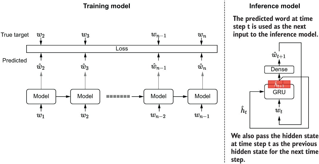
Figure 10.5 Comparison between the language model at training time and the inference/decoding phrase. In the inference phase, we predict one time step at a time. In each time step, we get the predicted word as the input and the new hidden state as the previous hidden state for the next time step.
We will use the Keras functional API to build this model, as shown in the next listing. First, let’s define two inputs.
Listing 10.6 Implementation of the inference/decoding language model
inp = tf.keras.layers.Input(shape=(None,))                                 ❶
inp_state = tf.keras.layers.Input(shape=(1024,))                           ❷

emb_layer = tf.keras.layers.Embedding(
    input_dim=n_vocab+1, output_dim=512, input_shape=(None,)
)                                                                          ❸
emb_out = emb_layer(inp)                                                   ❹

gru_layer = tf.keras.layers.GRU(
    1024, return_state=True, return_sequences=True
)
gru_out, gru_state = gru_layer(emb_out, initial_state=inp_state)         ❺❻

dense_layer = tf.keras.layers.Dense(512, activation='relu')                ❼
dense_out = dense_layer(gru_out)                                           ❼

final_layer = tf.keras.layers.Dense(n_vocab, name='final_out')             ❽
final_out = final_layer(dense_out)                                         ❽
softmax_out = tf.keras.layers.Activation(activation='softmax')(final_out)  ❽

infer_model = tf.keras.models.Model(
    inputs=[inp, inp_state], outputs=[softmax_out, gru_state]
)                                                                          ❾
❶ Define an input that can take an arbitrarily long sequence of word IDs.
❷ Define another input that will feed in the previous state.
❹ Get the embedding vectors from the input word ID.
❺ Define a GRU layer that returns both the output and the state. However, note that they will be the same for a GRU.
❻ Get the GRU output and the state from the model.
❼ Compute the first fully connected layer output.
❽ Define a final layer that is the same size as the vocabulary and get the final output of the model.
❾ Define the final model that takes an input and a state vector as the inputs and produces the next word prediction and the new state vector as the outputs.
We have to perform an important step after defining the model. We must transfer the weights from the trained model to the newly defined inference model. For that, we have to identify layers with trainable weights, get the weights for those layers from the trained model, and assign them to the new model:
# Copy the weights from the original model
emb_layer.set_weights(model.get_layer('embedding').get_weights())
gru_layer.set_weights(model.get_layer('gru').get_weights())
dense_layer.set_weights(model.get_layer('dense').get_weights())
final_layer.set_weights(model.get_layer('final_out').get_weights())
To get weights of a specific layer in the trained model, you can call
model.get_layer(<layer name>).get_weights()
This will return a NumPy array with the weights. Next, to assign those weights to a layer, call
layer.set_weights(<weight matrix>)
We can now call the newly defined model recursively to generate as many bigrams as we like. We will discuss the process to do that in more detail. Instead of starting with a single random word, let’s start with a sequence of text. We will convert the text to bigrams and subsequently to word IDs using the Tokenizer:
text = get_ngrams(
    "CHAPTER I. Down the Rabbit-Hole Alice was beginning to get very tired
➥ of sitting by her sister on the bank ,".lower(),
    ngrams
)

seq = tokenizer.texts_to_sequences([text])
Next, let’s reset the states of the model (this is not needed here because we’re starting fresh, but it’s good to know that we can do that). We will define a state vector with all zeros:
# Reset the state of the model initially
model.reset_states()
# Defining the initial state as all zeros
state = np.zeros(shape=(1,1024))
Then we will recursively predict on each bigram in the seq variable to update the state of the GRU model with the input sequence. Once we sweep through the whole sequence, we will get the final predicted bigram (that will be our first predicted bigram) and append that to the original bigram sequence:
# Recursively update the model by assining new state to state
for c in seq[0]:
    out, state = infer_model.predict([np.array([[c]]), state])

# Get final prediction after feeding the input string
wid = int(np.argmax(out[0],axis=-1).ravel())
word = tokenizer.index_word[wid]
text.append(word)
We will define a new input x with the last word ID that was predicted:
# Define first input to generate text recursively from
x = np.array([[wid]])
The fun begins now. We will predict 500 bigrams (i.e., 1,000 characters) using the approach discussed earlier. In every iteration, we predict a new bigram and the new state with the infer_model using the input x and the state vector state. The new bigram and the new state recursively replace x and state variables with these new outputs (see the next listing).
Listing 10.7 Recursively predicting a new word using the previous word as an input
for _ in range(500):

    out, state = infer_model.predict([x, state])                   ❶

    out_argsort = np.argsort(out[0], axis=-1).ravel()              ❷
    wid = int(out_argsort[-1])                                     ❷
    word = tokenizer.index_word[wid]                               ❷


    if word.endswith(' '):                                         ❸
        if np.random.normal()>0.5:
            width = 3                                              ❹
            i = np.random.choice(                                  ❹
                list(range(-width,0)),
                p=out_argsort[-width:]/out_argsort[-width:].sum()
            )
            wid = int(out_argsort[i])                              ❹
            word = tokenizer.index_word[wid]                       ❹
    text.append(word)                                              ❺

    x = np.array([[wid]])                                          ❻
❶ Get the next output and state.
❷ Get the word ID and the word from out.
❸ If the word ends with space, we introduce a bit of randomness to break repeating text.
❹ Essentially pick one of the top three outputs for that timestep depending on their likelihood.
❺ Append the prediction cumulatively to text.
❻ Recursively make the current prediction the next input.
Note that a little bit of work is required to get the final value of x as the model predicts a probability prediction (assigned to out) as its output, not a word ID. Furthermore, we’re going to use some additional logic to improve the randomness (or entropy, one could say) in the generated text by picking a word randomly from the top three words. But we don’t pick them with equal probability. Rather, let’s use their predicted probabilities to predict the word. To make sure we don’t get too much randomness and to avoid getting random tweaks in the middle of words, let’s do this only when the last character is a space character. The final word ID (picked either as the word with the highest probability or at random) is assigned to the variable x. This process will repeat for 500 steps, and by the end, you’ll have a cool machine-generated story on your hands. You can print the final text and see how it looks. To do that, simply join the bigrams in the text sequence as follows:
# Print the final output
print('
')
print('='*60)
print("Final text: ")
print(''.join(text))Final text: chapter i. down the rabbit-hole alice was beginning to get very tired of ➥ sitting by her sister on the bank , and then they went to the shore , ➥ and then the princess was so stilling that he was a little girl , ... it 's all right , and i 'll tell you how young things would n't be able to ➥ do it . i 'm not goin ' to think of itself , and i 'm going to be sure to see you . i 'm sure i can notice them . i 'm going to see you again , and i 'll tell you what i 've got , '
It’s certainly not bad for a simple single layer GRU model. Most of the time, the model spits out actual words. But there are occasional spelling mistakes and more frequent grammatical errors haunting the text. Can we do better? In the next section, we are going to learn about a new technique to generate text called beam search.
Assume you have the following code that chooses the next word greedily without randomness. You run this code and realize that the results are very bad:
for _ in range(500):

    out, new_s = infer_model.predict([x, s])

    out_argsort = np.argsort(out[0], axis=-1).ravel()
    wid = int(out_argsort[-1])
    word = tokenizer.index_word[wid]

    text.append(word)

    x = np.array([[wid]])
What do you think is the reason for the poor performance?
10.6 Beam search: Enhancing the predictive power of sequential models
We can do better that greedy decoding. Beam search is a popular decoding algorithm used in sequential/time-series tasks like this to generate more accurate predictions. The idea behind beam search is very simple. Unlike in greedy decoding, where you predict a single timestep, with beam search you predict several time steps ahead. In each time step, you get the top k predictions and branch out from them. Beam search has two important parameters: beam width and beam depth. Beam width controls how many candidates are considered at each step, whereas beam depth determines how many steps to search. For example, for a beam width of 3 and a beam depth of 5, the number of possible options become 35 = 243. Figure 10.6 further illustrates how beam search works.

Figure 10.6 Beam search in action. Beam search leads to better solutions as it looks several steps into the future to make a prediction. Here, we are performing a beam search with beam width = 3 and beam depth = 5.
First let’s define a function that will take a model, input, and state and return the output and the new state:
def beam_one_step(model, input_, state):
    """ Perform the model update and output for one step"""
    output, new_state = model.predict([input_, state])
    return output, new_state
Then, using this function, we will define a recursive function (recursive_fn) that will recursively predict the next word from the previous prediction for a predefined depth (defined by beam_depth). At each time step, we consider the top k candidates (defined by beam_width) to branch out from. The recursive_fn function will populate a variable called results. results will contain a list of tuples, where each tuple represents a single path in the search. Specifically, each tuple contains the
This function is outlined in the following listing.
Listing 10.8 Implementation of the beam search as a recursive function
def beam_search(
    model, input_, state, beam_depth=5, beam_width=3, ignore_blank=True
):                                                                           ❶
    """ Defines an outer wrapper for the computational function of beam
➥ search """

    def recursive_fn(input_, state, sequence, log_prob, i):                  ❷
        """ This function performs actual recursive computation of the long
➥ string"""

        if i == beam_depth:                                                  ❸
            """ Base case: Terminate the beam search """
            results.append((list(sequence), state, np.exp(log_prob)))        ❹
            return sequence, log_prob, state                                 ❹
        else:
            """ Recursive case: Keep computing the output using the
➥ previous outputs"""
            output, new_state = beam_one_step(model, input_, state)          ❺

            # Get the top beam_widht candidates for the given depth
            top_probs, top_ids = tf.nn.top_k(output, k=beam_width)           ❻
            top_probs, top_ids = top_probs.numpy().ravel(),
➥ top_ids.numpy().ravel()                                                   ❻

            # For each candidate compute the next prediction
            for p, wid in zip(top_probs, top_ids):                           ❼
                new_log_prob = log_prob + np.log(p)                          ❼
                if len(sequence)>0 and wid == sequence[-1]:                  ❽
                    new_log_prob = new_log_prob + np.log(1e-1)               ❽

                sequence.append(wid)                                         ❾
                _ = recursive_fn(
                    np.array([[wid]]), new_state, sequence, new_log_prob, i+1❿
                )
                sequence.pop()

    results = []
    sequence = []
    log_prob = 0.0
    recursive_fn(input_, state, sequence, log_prob, 0)                       ⓫

    results = sorted(results, key=lambda x: x[2], reverse=True)              ⓬

    return results
❶ Define an outer wrapper for the computational function of beam search.
❷ Define an inner function that is called recursively to find the beam paths.
❸ Define the base case for terminating the recursion.
❹ Append the result we got at the termination so we can use it later.
❺ During recursion, get the output word and the state by calling the model.
❻ Get the top k candidates for that step.
❼ For each candidate, compute the joint probability. We will do this in log space to have numerical stability.
❽ Penalize joint probability whenever the same symbol repeats.
❾ Append the current candidate to the sequence that maintains the current search path at the time.
❿ Call the function recursively to find the next candidates.
⓫ Make a call to the recursive function to trigger the recursion.
⓬ Sort the results by log probability.
Finally, we can use this beam_search function as follows: we will use a beam depth of 7 and a beam width of 2. Up until the for loop, things are identical to how we did things using greedy decoding. In the for loop, we get the results list (sorted high to low on joint probability). Then, similar to what we did previously, we’ll get the next prediction randomly from the top 10 predictions based on their likelihood as the next prediction. The following listing delineates the code to do so.
Listing 10.9 Implementation of beam search decoding to generate a new story
text = get_ngrams(
    "CHAPTER I. Down the Rabbit-Hole Alice was beginning to get very tired
➥ of sitting by her sister on the bank ,".lower(),
    ngrams
)                                                                ❶

seq = tokenizer.texts_to_sequences([text])                       ❷

state = np.zeros(shape=(1,1024))
for c in seq[0]:
    out, state = infer_model.predict([np.array([[c]]), state     ❸

wid = int(np.argmax(out[0],axis=-1).ravel())                     ❹
word = tokenizer.index_word[wid]                                 ❹
text.append(word)                                                ❹

x = np.array([[wid]])

for i in range(100):                                             ❺

    result = beam_search(infer_model, x, state, 7, 2)            ❻

    n_probs = np.array([p for _,_,p in result[:10                ❼
    p_j = np.random.choice(list(range(
       n_probs.size)), p=n_probs/n_probs.sum())                  ❼

    best_beam_ids, state, _ = result[p_j]                        ❽
    x = np.array([[best_beam_ids[-1]]])                          ❽

    text.extend([tokenizer.index_word[w] for w in best_beam_ids])

print('
')
print('='*60)
print("Final text: ")
print(''.join(text))
❶ Define a sequence of ngrams from an initial sequence of text.
❷ Convert the bigrams to word IDs.
❸ Build up model state using the given string.
❹ Get the predicted word after processing the sequence.
❻ Get the results from beam search.
❼ Get one of the top 10 results based on their likelihood.
❽ Replace x and state with the new values computed.
Running the code in listing 10.9, you should get text similar to the following:
Final text:

chapter i. down the rabbit-hole alice was beginning to get very tired of
➥ sitting by her sister on the bank , and there was no reason that her
➥ father had brought him the story girl 's face .
 `` i 'm going to bed , '' said the prince , `` and you can not be able
➥ to do it . ''
 `` i 'm sure i shall have to go to bed , '' he answered , with a smile
➥ .
 `` i 'm so happy , '' she said .
 `` i do n't know how to bring you into the world , and i 'll be sure
➥ that you would have thought that it would have been a long time .
 there was no time to be able to do it , and it would have been a
➥ little thing . ''
 `` i do n't know , '' she said .

...

 `` what is the matter ? ''
 `` no , '' said anne , with a smile .
 `` i do n't know what to do , '' said mary .
 `` i 'm so glad you come back , '' said mrs. march , with
The text generated with beam search reads much better than the text we saw with greedy decoding. You see improved grammar and less spelling mistakes when text is generated with beam search.
This concludes our discussion on language modeling. In the next chapter, we will learn about a new type of NLP problem known as a sequence-to-sequence problem. Let’s summarize the key highlights of this chapter.
You used the line result = beam_search(infer_model, x, state, 7, 2) to perform beam search. You want to consider five candidates at a given time and search only three levels deep into the search space. How would you change the line?
Summary
-
Language modeling is the task of predicting the next word given a sequence of words.
-
Language modeling is the workhorse of some of the top-performing models in the field, such as BERT (a type of Transformer-based model).
-
To limit the size of the vocabulary and avoid computational issues, n-gram representation can be used.
-
In n-gram representation, text is split into fixed-length tokens, as opposed to doing character-level or word-level tokenization. Then, a fixed sized window is moved over the sequence of text to generate inputs and targets for the model. In TensorFlow, you can use the tf.data.Dataset.window() function to implement this functionality.
-
The gated recurrent unit (GRU) is a sequential model that operates similarly to an LSTM, where it jumps from one input to the next in a sequence while generating a state at each time step.
-
The GRU is a compact version of an LSTM model that maintains a single state and two gates but delivers on-par performance.
-
Perplexity measures how surprised the model was to see the target word given the input sequence.
-
The computation of the perplexity measure is inspired by information theory, in which the measure entropy is used to quantify the uncertainty in a random variable that represents an event where the outcomes are generated with some underlying probability distribution.
-
The language models after training can be used to generate new text. There are two popular techniques—greedy decoding and beam search decoding:
Answers to exercises
ds = tf.data.Dataset.from_tensor_slices(x)
ds = ds.window(5,shift=5).flat_map(
    lambda window: window.batch(5, drop_remainder=True)
)
ds = ds.map(lambda xx: (xx[:-2], xx[2:]))model = tf.keras.models.Sequential([
tf.keras.layers.Embedding(
input_dim=n_vocab+1, output_dim=512,input_shape=(None,)
),
tf.keras.layers.GRU(1024, return_state=False, return_sequences=True),
tf.keras.layers.GRU(512, return_state=False, return_sequences=True),
tf.keras.layers.Dense(n_vocab, activation=’softmax’, name='final_out'),
])Scenario A will have the lowest perplexity.
es_callback = tf.keras.callbacks.EarlyStopping(
    monitor=’val_accuracy’, patience=5, mode=’max’, restore_best_weights=False
)The line out, new_s = infer_model.predict([x, s]), is wrong. The state is not recursively updated in the inference model. This will lead to a working model but with poor performance. It should be corrected as out, s = infer_model.predict([x, s]).
result = beam_search(infer_model, x, state, 3, 5)