
16
Futures, Scheduling, and Work Distribution
16.1 Introduction
In this chapter we show how to decompose certain kinds of problems into components that can be executed in parallel. Some applications break down naturally into parallel threads. For example, when a request arrives at a web server, the server can just create a thread (or assign an existing thread) to handle the request. Applications that can be structured as producers and consumers also tend to be easily parallelizable. In this chapter, however, we look at applications that have inherent parallelism, but where it is not obvious how to take advantage of it.
Let us start by thinking about how to multiply two matrices in parallel. Recall that if aij is the value at position (i,j) of matrix A, then the product C of two n × n matrices A and B is given by:
![]()
As a first step, we could put one thread in charge of computing each cij. Fig. 16.1 shows a matrix multiplication program that creates an n × n array of Worker threads (Fig. 16.2), where the worker thread in position (i,j) computes cij. The program starts each task, and waits for them all to finish.1

Figure 16.1 The MMThread task: matrix multiplication using threads.
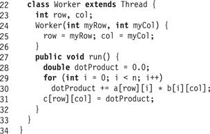
Figure 16.2 The MMThread task: inner Worker thread class.
In principle, this might seem like an ideal design. The program is highly parallel, and the threads do not even have to synchronize. In practice, however, while this design might perform well for small matrices, it would perform very poorly for matrices large enough to be interesting. Here is why: threads require memory for stacks and other bookkeeping information. Creating, scheduling, and destroying threads takes a substantial amount of computation. Creating lots of short-lived threads is an inefficient way to organize a multi-threaded computation.
A more effective way to organize such a program is to create a pool of long-lived threads. Each thread in the pool repeatedly waits until it is assigned a task, a short-lived unit of computation. When a thread is assigned a task, it executes that task, and then rejoins the pool to await its next assignment. Thread pools can be platform-dependent: it makes sense for large-scale multiprocessors to provide large pools, and vice versa. Thread pools avoid the cost of creating and destroying threads in response to short-lived fluctuations in demand.
In addition to performance benefits, thread pools have another equally important, but less obvious advantage: they insulate the application programmer from platform-specific details such as the number of concurrent threads that can be scheduled efficiently. Thread pools make it possible to write a single program that runs equally well on a uniprocessor, a small-scale multiprocessor, and a large-scale multiprocessor. They provide a simple interface that hides complex, platform-dependent engineering trade-offs.
In Java, a thread pool is called an executor service (interface java.util.ExecutorService). It provides the ability to submit a task, the ability to wait for a set of submitted tasks to complete, and the ability to cancel uncompleted tasks. A task that does not return a result is usually represented as a Runnable object, where the work is performed by a run() method that takes no arguments and returns no results. A task that returns a value of type T is usually represented as a Callable<T> object, where the result is returned by a call() with the T method that takes no arguments.
When a Callable<T> object is submitted to an executor service, the service returns an object implementing the Future<T> interface. A Future<T> is a promise to deliver the result of an asynchronous computation, when it is ready. It provides a get() method that returns the result, blocking if necessary until the result is ready. (It also provides methods for canceling uncompleted computations, and for testing whether the computation is complete.) Submitting a Runnable task also returns a future. Unlike the future returned for a Callable<T> object, this future does not return a value, but the caller can use that future’s get() method to block until the computation finishes. A future that does not return an interesting value is declared to have class Future<?>.
It is important to understand that creating a future does not guarantee that any computations actually happen in parallel. Instead, these methods are advisory: they tell an underlying executor service that it may execute these methods in parallel.
We now consider how to implement parallel matrix operations using an executor service. Fig. 16.3 shows a Matrix class that provides put() and get() methods to access matrix elements, along with a constant-time split() method that splits an n-by-n matrix into four (n/2)-by-(n/2) submatrices. In Java terminology, the four submatrices are backed by the original matrix, meaning that changes to the submatrices are reflected in the original, and vice versa.
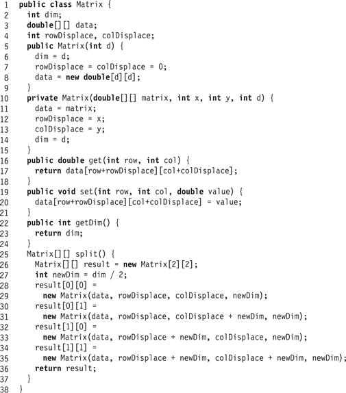
Figure 16.3 The Matrix class.
Our job is to devise a MatrixTask class that provides parallel methods to add and multiply matrices. This class has one static field, an executor service called exec, and two static methods to add and multiply matrices.
For simplicity, we consider matrices whose dimension n is a power of 2. Any such matrix can be decomposed into four submatrices:
![]()
Matrix addition C = A + B can be decomposed as follows:
These four sums can be done in parallel.
The code for multithreaded matrix addition appears in Fig. 16.4. The AddTask class has three fields, initialized by the constructor: a and b are the matrices to be summed, and c is the result, which is updated in place. Each task does the following. At the bottom of the recursion, it simply adds the two scalar values (Line 20 of Fig. 16.4).2 Otherwise, it splits each of its arguments into four sub-matrices (Line 22), and launches a new task for each sub-matrix (Lines 24–27). Then, it waits until all futures can be evaluated, meaning that the sub-computations have finished (Lines 28–30). At that point, the task simply returns, the result of the computation having been stored in the result matrix. Matrix multiplication C = A ⋅ B can be decomposed as follows:

The eight product terms can be computed in parallel, and when those computations are done, the four sums can then be computed in parallel.
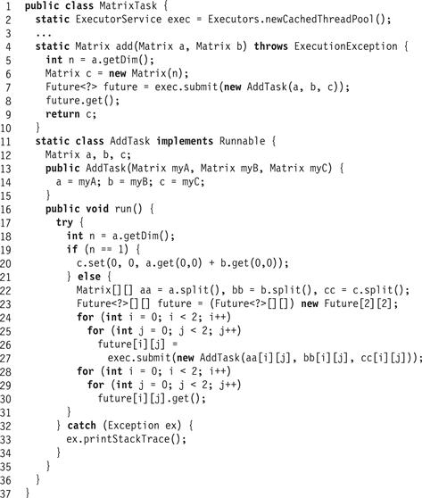
Figure 16.4 The MatrixTask class: parallel matrix addition.
Fig. 16.5 shows the code for the parallel matrix multiplication task. Matrix multiplication is structured in a similar way to addition. The MulTask class creates two scratch arrays to hold the matrix product terms (Line 42). It splits all five matrices (Line 50), submits tasks to compute the eight product terms in parallel (Line 56), and waits for them to complete (Line 60). Once they are complete, the thread submits tasks to compute the four sums in parallel (Line 64), and waits for them to complete (Line 65).

Figure 16.5 The MatrixTask class: parallel matrix multiplication.
The matrix example uses futures only to signal when a task is complete. Futures can also be used to pass values from completed tasks. To illustrate this use of futures, we consider how to decompose the well-known Fibonacci function into a multithreaded program. Recall that the Fibonacci sequence is defined as follows:

Fig. 16.6 shows one way to compute Fibonacci numbers in parallel. This implementation is very inefficient, but we use it here to illustrate multithreaded dependencies. The call() method creates two futures, one that computes F(n − 2) and another that computes F(n − 1), and then sums them. On a multiprocessor, time spent blocking on the future for F(n − 1) can be used to compute F(n − 2).

Figure 16.6 The FibTask class: a Fibonacci task with futures.
16.2 Analyzing Parallelism
Think of a multithreaded computation as a directed acyclic graph (DAG), where each node represents a task, and each directed edge links a predecessor task to a successor task, where the successor depends on the predecessor’s result. For example, a conventional thread is just a chain of nodes where each node depends on its predecessor. By contrast, a node that creates a future has two successors: one node is its successor in the same thread, and the other is the first node in the future’s computation. There is also an edge in the other direction, from child to parent, that occurs when a thread that has created a future calls that future’s get() method, waiting for the child computation to complete. Fig. 16.7 shows the DAG corresponding to a short Fibonacci execution.

Figure 16.7 The DAG created by a multithreaded Fibonacci execution. The caller creates a FibTask(4) task, which in turn creates FibTask(3) and FibTask(2) tasks. The round nodes represent computation steps and the arrows between the nodes represent dependencies. For example, there are arrows pointing from the first two nodes in FibTask(4) to the first nodes in FibTask(3) and FibTask(2) respectively, representing submit() calls, and arrows from the last nodes in FibTask(3) and FibTask(2) to the last node in FibTask(4) representing get() calls. The computation’s critical path has length 8 and is marked by numbered nodes.
Some computations are inherently more parallel than others. Let us make this notion precise. Assume that all individual computation steps take the same amount of time, which constitutes our basic measuring unit. Let TP be the minimum time (measured in computation steps) needed to execute a multithreaded program on a system of P dedicated processors. TP is thus the program’s latency, the time it would take it to run from start to finish, as measured by an outside observer. We emphasize that TP is an idealized measure: it may not always be possible for every processor to find steps to execute, and actual computation time may be limited by other concerns, such as memory usage. Nevertheless, TP is clearly a lower bound on how much parallelism one can extract from a multithreaded computation.
Some values of T are important enough that they have special names. T1, the number of steps needed to execute the program on a single processor, is called the computation’s work. Work is also the total number of steps in the entire computation. In one time step (of the outside observer), P processors can execute at most P computation steps, so
![]()
The other extreme is also of special importance: T∞, the number of steps to execute the program on an unlimited number of processors, is called the critical-path length. Because finite resources cannot do better than infinite resources,
![]()
The speedup on P processors is the ratio:
![]()
We say a computation has linear speedup if T1/TP = Θ(P). Finally, a computation’sparallelism is the maximum possible speedup: T1/T∞. A computation’s parallelism is also the average amount of work available at each step along the critical path, and so provides a good estimate of the number of processors one should devote to a computation. In particular, it makes little sense to use substantially more than that number of processors.
To illustrate these concepts, we now revisit the concurrent matrix add and multiply implementations introduced in Section 16.1.
Let AP(n) be the number of steps needed to add two n × n matrices on P processors. Recall that matrix addition requires four half-size matrix additions, plus a constant amount of work to split the matrices. The work A1(n) is given by the recurrence:
![]()
This program has the same work as the conventional doubly-nested loop implementation.
Because the half-size additions can be done in parallel, the critical path length is given by the following formula.
![]()
Let MP(n) be the number of steps needed to multiply two n × n matrices on P processors. Recall that matrix multiplication requires eight half-size matrix multiplications and four matrix additions. The work M1(n) is given by the recurrence:

This work is also the same as the conventional triply-nested loop implementation. The half-size multiplications can be done in parallel, and so can the additions, but the additions must wait for the multiplications to complete. The critical path length is given by the following formula:

The parallelism for matrix multiplication is given by:
![]()
which is pretty high. For example, suppose we want to multiply two 1000-by-1000 matrices. Here, n3 = 109, and log n = log 1000 ≈ 10 (logs are base two), so the parallelism is approximately 109/102 = 107. Roughly speaking, this instance of matrix multiplication could, in principle, keep roughly a million processors busy well beyond the powers of any multiprocessor we are likely to see in the immediate future.
We should understand that the parallelism in the computation given here is a highly idealized upper bound on the performance of any multithreaded matrix multiplication program. For example, when there are idle threads, it may not be easy to assign those threads to idle processors. Moreover, a program that displays less parallelism but consumes less memory may perform better because it encounters fewer page faults. The actual performance of a multithreaded computation remains a complex engineering problem, but the kind of analysis presented in this chapter is an indispensable first step in understanding the degree to which a problem can be solved in parallel.
16.3 Realistic Multiprocessor Scheduling
Our analysis so far has been based on the assumption that each multithreaded program has P dedicated processors. This assumption, unfortunately, is not realistic. Multiprocessors typically run a mix of jobs, where jobs come and go dynamically. One might start, say, a matrix multiplication application on P processors. At some point, the operating system may decide to download a new software upgrade, preempting one processor, and the application then runs on P − 1 processors. The upgrade program pauses waiting for a disk read or write to complete, and in the interim the matrix application has P processors again.
Modern operating systems provide user-level threads that encompass a program counter and a stack. (A thread that includes its own address space is often called a process.) The operating system kernel includes a scheduler that runs threads on physical processors. The application, however, typically has no control over the mapping between threads and processors, and so cannot control when threads are scheduled.
As we have seen, one way to bridge the gap between user-level threads and operating system-level processors is to provide the software developer with a three-level model. At the top level, multithreaded programs (such as matrix multiplication) decompose an application into a dynamically-varying number of short-lived tasks. At the middle level, a user-level scheduler maps these tasks to a fixed number of threads. At the bottom level, the kernel maps these threads onto hardware processors, whose availability may vary dynamically. This last level of mapping is not under the application’s control: applications cannot tell the kernel how to schedule threads (especially because commercially available operating systems kernels are hidden from users).
Assume for simplicity that the kernel works in discrete steps: at step i, the kernel chooses an arbitrary subset of 0 ≤ pi ≤ P user-level threads to run for one step. The processor average PA over T steps is defined to be:
![]() 16.3.1
16.3.1
Instead of designing a user-level schedule to achieve a P-fold speedup, we can try to achieve a PA-fold speedup. A schedule is greedy if the number of program steps executed at each time step is the minimum of pi, the number of available processors, and the number of ready nodes (ones whose associated step is ready to be executed) in the program DAG. In other words, it executes as many of the ready nodes as possible, given the number of available processors.
Theorem 16.3.1
Consider a multithreaded program with work T1, critical-path length T∞, and P user-level threads. We claim that any greedy execution has length T which is at most
![]()
Proof
Equation 16.3.1 implies that:
![]()
We bound T by bounding the sum of the pi. At each kernel-level step i, let us imagine getting a token for each thread that was assigned a processor. We can place these tokens in one of two buckets. For each user-level thread that executes a node at step i, we place a token in a work bucket, and for each thread that remains idle at that step (that is, it was assigned to a processor but was not ready to execute because the node associated with its next step had dependencies that force it to wait for some other threads), we place a token in an idle bucket. After the last step, the work bucket contains T1 tokens, one for each node of the computation DAG. How many tokens does the idle bucket contain?
We define an idle step as one in which some thread places a token in the idle bucket. Because the application is still running, at least one node is ready for execution in each step. Because the scheduler is greedy, at least one node will be executed, so at least one processor is not idle. Thus, of the pi threads scheduled at step i, at most pi − 1 ≤ P − 1 can be idle.
How many idle steps could there be? Let Gi be a sub-DAG of the computation consisting of the nodes that have not been executed at the end of step i. Every node that does not have incoming edges (apart from its predecessor in program order) in Gi−1 (such as the last node of FibTask(2) at the end of step 6) was ready at the start of step i. There must be fewer than pi such nodes, because otherwise the greedy schedule could execute pi of them, and the step i would not be idle. Thus, the scheduler must have executed this step. It follows that the longest directed path in Gi is one shorter than the longest directed path in Gi−1. The longest directed path before step 0 is T∞, so the greedy schedule can have at most T∞ idle steps. Combining these observations we deduce that at most T∞ idle steps are executed with at most (P − 1) tokens added in each, so the idle bucket contains at most T∞(P − 1) tokens.
The total number of tokens in both buckets is therefore
![]()
yielding the desired bound.
It turns out that this bound is within a factor of two of optimal. Actually, achieving an optimal schedule is NP-complete, so greedy schedules are a simple and practical way to achieve performance that is reasonably close to optimal.
16.4 Work Distribution
We now understand that the key to achieving a good speedup is to keep user-level threads supplied with tasks, so that the resulting schedule is as greedy as possible. Multithreaded computations, however, create and destroy tasks dynamically, sometimes in unpredictable ways. A work distribution algorithm is needed to assign ready tasks to idle threads as efficiently as possible.
One simple approach to work distribution is work dealing: an overloaded thread tries to offload tasks to other, less heavily loaded threads. This approach may seem sensible, but it has a basic flaw: if most threads are overloaded, then they waste effort in a futile attempt to exchange tasks.
Instead, we first consider work stealing, in which a thread that runs out of work tries to “steal” work from others. An advantage of work stealing is that if all threads are already busy, then they do not waste time trying to offload work on one another.
16.4.1 Work Stealing
Each thread keeps a pool of tasks waiting to be executed in the form of a double-ended queue (DEQueue), providing pushBottom(), popBottom(), and popTop() methods (there is no need for a pushTop() method). When a thread creates a new task, it calls pushBottom() to push that task onto its DEQueue. When a thread needs a task to work on, it calls popBottom() to remove a task from its own DEQueue. If the thread discovers its queue is empty, then it becomes a thief: it chooses a victim thread at random, and calls that thread’s DEQueue’s popTop() method to “steal” a task for itself.
In Section 16.5 we devise an efficient linearizable implementation of a DEQueue. Fig. 16.8 shows one possible way to implement a thread used by a work-stealing executor service. The threads share an array of DEQueues (Line 2), one for each thread. Each thread repeatedly removes a task from its own DEQueue and runs it (Lines 12–15). If it runs out, then it repeatedly chooses a victim thread at random and tries to steal a task from the top of the victim’s DEQueue (Lines 16–22). To avoid code clutter, we ignore the possibility that stealing may trigger an exception.

Figure 16.8 The WorkStealingThread class: a simplified work stealing executer pool.
This simplified executer pool may keep trying to steal forever, long after all work in all queues has been completed. To prevent threads from endlessly searching for nonexistent work, we can use a termination-detecting barrier of the kind described in Chapter 17, section 17.6.
16.4.2 Yielding and Multiprogramming
As noted earlier, multiprocessors provide a three-level model of computation: short-lived tasks are executed by system-level threads, which are scheduled by the operating system on a fixed number of processors. A multiprogrammed environment is one in which there are more threads than processors, implying that not all threads can run at the same time, and that any thread can be preemptively suspended at any time. To guarantee progress, we must ensure that threads that have work to do are not unreasonably delayed by (thief) threads which are idle except for task-stealing. To prevent this situation, we have each thief call Thread.yield() immediately before trying to steal a task (Line 17 in Fig. 16.8). This call yields the thief’s processor to another thread, allowing descheduled threads to regain a processor and make progress. (We note that calling yield() has no effect if there are no descheduled threads capable of running.)
16.5 Work-Stealing Dequeues
Here is how to implement a work-stealing DEQueue. Ideally, a work-stealing algorithm should provide a linearizable implementation whose pop methods always return a task if one is available. In practice, however, we can settle for something weaker, allowing a popTop() call to return null if it conflicts with a concurrent popTop() call. Though we could have the unsuccessful thief simply try again, it makes more sense in this context to have a thread retry the popTop() operation on a different, randomly chosen DEQueue each time. To support such a retry, a popTop() call may return null if it conflicts with a concurrent popTop() call.
We now describe two implementations of the work-stealing DEQueue. The first is simpler, because it has bounded capacity. The second is somewhat more complex, but virtually unbounded in its capacity; that is, it does not suffer from the possibility of overflow.
16.5.1 A Bounded Work-Stealing Dequeue
For the executer pool DEQueue, the common case is for a thread to push and pop a task from its own queue, calling pushBottom() and popBottom(). The uncommon case is to steal a task from another thread’s DEQueue by calling popTop(). Naturally, it makes sense to optimize the common case. The idea behind the BoundedDEQueue in Figs. 16.9 and 16.10 is thus to have the pushBottom() and popBottom() methods use only reads–writes in the common case. The BoundedDEQueue consists of an array of tasks indexed by bottom and top fields that reference the bottom and top of the dequeue, and depicted in Fig. 16.11. The pushBottom() and popBottom() methods use reads–writes to manipulate the bottom reference. However, once the top and bottom fields are close (there might be only a single item in the array), popBottom() switches to compareAndSet() calls to coordinate with potential popTop() calls.

Figure 16.9 The BDEQueue class: fields, constructor, pushBottom() and isEmpty() methods.
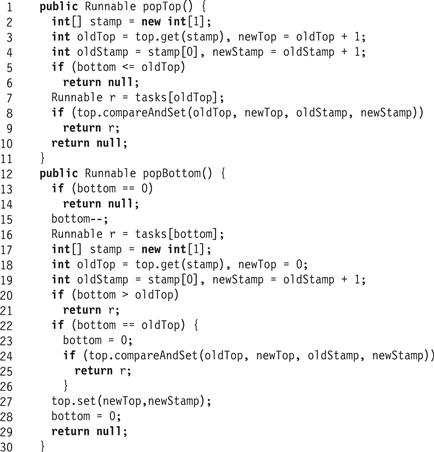
Figure 16.10 The BoundedDEQueue class: popTop() and popBottom() methods.

Figure 16.11 The BoundedDEQueue implementation. In Part (a) popTop() and popBottom() are called concurrently while there is more than one task in the BoundedDEQueue. The popTop() method reads the element in entry 2 and calls compareAndSet() to redirect the top reference to entry 3. The popBottom() method redirects the bottom reference from 5 to 4 using a simple store and then, after checking that bottom is greater than top it removes the task in entry 4. In Part (b) there is only a single task. When popBottom() detects that after redirecting from 4 to 3 top and bottom are equal, it attempts to redirect top with a compareAndSet(). Before doing so it redirects bottom to 0 because this last task will be removed by one of the two popping methods. If popTop() detects that top and bottom are equal it gives up, and otherwise it tries to advance top using compareAndSet(). If both methods apply compareAndSet() to the top, one wins and removes the task. In any case, win or lose, popBottom() resets top to 0 since the BoundedDEQueue is empty.
Let us describe the algorithm in more detail. The BoundedDEQueue algorithm is ingenious in the way it avoids the use of costly compareAndSet() calls. This elegance comes at a cost: it is delicate and the order among instructions is crucial. We suggest the reader take time to understand how method interactions among methods are determined by the order in which reads-writes and compareAndSet() calls occur.
The BoundedDEQueue class has three fields: tasks, bottom, and top (Fig. 16.9, Lines 2–4). The tasks field is an array of Runnable tasks that holds the tasks in the queue, bottom is the index of the first empty slot in tasks, and top is an AtomicStampedReference<Integer>.3 The top field encompasses two logical fields; the reference is the index of the first task in the queue, and the stamp is a counter incremented each time the reference is changed. The stamp is needed to avoid an “ABA” problem of the type that often arises when using compareAndSet(). Suppose thread A tries to steal a task from index 3. A reads a reference to the task at that position, and tries to steal it by calling compareAndSet() to set the index to 4. It is delayed before making the call, and in the meantime, thread B removes all the tasks and inserts three new tasks. When A awakens, its compareAndSet() call will succeed in changing the index from 3 to 4, but it will have stolen a task that has already been completed, and removed a task that will never be completed. The stamp ensures that A’s compareAndSet() call will fail because the stamps no longer match.
The popTop() method (Fig. 16.10) checks whether the BoundedDEQueue is empty, and if not, tries to steal the top element by calling compareAndSet() to increment top. If the compareAndSet() succeeds, the theft is successful, and otherwise the method simply returns null. This method is nondeterministic: returning null does not necessarily mean that the queue is empty.
As we noted earlier, we optimize for the common case where each thread pushes and pops from its own local BoundedDEQueue. Most of the time, a thread can push and pop tasks on and off its own BoundedDEQueue object, simply by loading and storing the bottom index. If there is only one task in the queue, then the caller might encounter interference from a thief trying to steal that task. So if bottom is close to top, the calling thread switches to using compareAndSet() to pop tasks.
The pushBottom() method (Fig. 16.9, Line 10) simply stores the new task at the bottom queue location and increments bottom.
The popBottom() method (Fig. 16.10) is more complex. If the queue is empty, the method returns immediately (Line 13), and otherwise, it decrements bottom, claiming a task (Line 15). Here is a subtle but important point. If the claimed task was the last in the queue, then it is important that thieves notice that the BoundedDEQueue is empty (Line 5). But, because popBottom()’s decrement is neither atomic nor synchronized, the Java memory model does not guarantee that the decrement will be observed right away by concurrent thieves. To ensure that thieves can recognize an empty BoundedDEQueue, the bottom field must be declared volatile.4
After the decrement, the caller reads the task at the new bottom index (Line 16), and tests whether the current top field refers to a higher index. If so, the caller cannot conflict with a thief, and the method returns (Line 20). Otherwise, if the top and bottom fields are equal, then there is only one task left in the BoundedDEQueue, but there is a danger that the caller conflicts with a thief. The caller resets bottom to 0 (Line 23). (Either the caller will succeed in claiming the task, or a thief will steal it first.) The caller resolves the potential conflict by calling compareAndSet() to reset top to 0, matching bottom (Line 22). If this compareAndSet() succeeds, the top has been reset to 0, and the task has been claimed by the caller, so the method returns. Otherwise the queue must be empty because a thief succeeded, but this means that top points to some entry greater than bottom which was set to 0 earlier. So before the caller returns null, it resets top to 0 (Line 27).
As noted, an attractive aspect of this design is that an expensive compareAndSet() call is needed only rarely when the BoundedDEQueue is almost empty.
We linearize each unsuccessful popTop() call at the point where it detects that the BoundedDEQueue is empty, or at a failed compareAndSet(). Successful popTop() calls are linearized at the point when a successful compareAndSet() took place. We linearize pushBottom() calls when bottom is incremented, and popBottom() calls when bottom is decremented or set to 0, though the outcome of popBottom() in the latter case is determined by the success or failure of the compareAndSet() that follows.
The isEmpty() method (Fig. 16.10) first reads top, then bottom, checking whether bottom is less than or equal to top (Line 4). The order is important for linearizability, because top never decreases unless bottom is first reset to 0, and so if a thread reads bottom after top and sees it is no greater, the queue is indeed empty because a concurrent modification of top could only have increased top. On the other hand, if bottom is greater than top, then even if top is increased after it was read and before bottom is read (and the queue becomes empty), it is still true that the BoundedDEQueue must not have been empty when top was read. The only alternative is that bottom is reset to 0 and then top is reset to 0, so reading top and then bottom will correctly return empty. It follows that the isEmpty() method is linearizable.
16.5.2 An Unbounded Work-Stealing DEQueue
A limitation of the BoundedDEQueue class is that the queue has a fixed size. For some applications, it may be difficult to predict this size, especially if some threads create significantly more tasks than others. Assigning each thread its own BoundedDEQueue of maximal capacity wastes space.
To address these limitations, we now consider an unbounded double-ended queue UnboundedDEQueue class that dynamically resizes itself as needed.
We implement the UnboundedDEQueue in a cyclic array, with top and bottom fields as in the BoundedDEQueue (except indexed modulo the array’s capacity). As before, if bottom is less than or equal to top, the UnboundedDEQueue is empty. Using a cyclic array eliminates the need to reset bottom and top to 0. Moreover, it permits top to be incremented but never decremented, eliminating the need for top to be an AtomicStampedReference. Moreover, in the UnboundedDEQueue algorithm, if pushBottom() discovers that the current circular array is full, it can resize (enlarge) it, copying the tasks into a bigger array, and pushing the new task into the new (larger) array. Because the array is indexed modulo its capacity, there is no need to update the top or bottom fields when moving the elements into a bigger array (although the actual array indexes where the elements are stored might change).
The CircularArray() class is depicted in Fig. 16.12. It provides get() and put() methods that add and remove tasks, and a resize method that allocates a new circular array and copies the old array’s contents into the new array. The use of modular arithmetic ensures that even though the array has changed size and the tasks may have shifted positions, thieves can still use the top field to find the next task to steal.

Figure 16.12 The UnboundedDEQueue class: the circular task array.
The UnboundedDEQueue class has three fields: tasks, bottom, and top (Fig. 16.13, Lines 3–5). The popBottom() (Fig. 16.13) and popTop() methods (Fig. 16.14) are almost the same as those of the BoundedDEQueue, with one key difference: the use of modular arithmetic to compute indexes means the top index need never be decremented. As noted, there is no need for a timestamp to prevent ABA problems. Both methods, when competing for the last task, steal it by incrementing top. To reset the UnboundedDEQueue to empty, simply increment the bottom field to equal top. In the code, popBottom(), immediately after the compareAndSet() in Line 25, sets bottom to equal top +1 whether or not the compareAndSet() succeeds, because, even if it failed, a concurrent thief must have stolen the last task. Storing top +1 into bottom makes top and bottom equal, resetting the UnboundedDEQueue object to an empty state.

Figure 16.13 The UnboundedDEQueue class: fields, constructor, pushBottom(), and isEmpty() methods.

Figure 16.14 The UnboundedDEQueue class: popTop() and popBottom() methods.
The isEmpty() method (Fig. 16.13) first reads top, then bottom, checking whether bottom is less than or equal to top (Line 4). The order is important because top never decreases, and so if a thread reads bottom after top and sees it is no greater, the queue is indeed empty because a concurrent modification of top could only have increased the top value. The same principle applies in the popTop() method call. An example execution is provided in Fig. 16.15.

Figure 16.15 The UnboundedDEQueue class implementation. In Part (a) popTop() and popBottom() are executed concurrently while there is more than one task in the UnboundedDEQueue object. In Part (b) there is only a single task, and initially bottom refers to Entry 3 and top to 2. The popBottom() method first decrements bottom from 3 to 2 (we denote this change by a dashed line pointing to Entry 2 since it will change again soon). Then, when popBottom() detects that the gap between the newly-set bottom and top is 0, it attempts to increment top by 1 (rather than reset it to 0 as in the BoundedDEQueue). The popTop() method attempts to do the same. The top field is incremented by one of them, and the winner takes the last task. Finally, the popBottom() method sets bottom back to Entry 3, which is equal to top.
The pushBottom() method (Fig. 16.13) is almost the same as that of the BoundedDEQueue. One difference is that the method must enlarge the circular array if the current push is about to cause it to exceed its capacity. Another is that popTop() does not need to manipulate a timestamp. The ability to resize carries a price: every call must read top (Line 20) to determine if a resize is necessary, possibly causing more cache misses because top is modified by all processes. We can reduce this overhead by having threads save a local value of top and using it to compute the size of the UnboundedDEQueue object. A thread reads the top field only when this bound is exceeded, indicating that a resize may be necessary. Even though the local copy may become outdated because of changes to the shared top, top is never decremented, so the real size of the UnboundedDEQueue object can only be smaller than the one calculated using the local variable.
In summary, we have seen two ways to design a nonblocking linearizable DEQueue class. We can get away with using only loads and stores in the most common manipulations of the DEQueue, but at the price of having more complex algorithms. Such algorithms are justifiable for an application such as an executer pool whose performance may be critical to a concurrent multithreaded system.
16.5.3 Work Balancing
We have seen that in work-stealing algorithms, idle threads steal tasks from others. An alternative approach is to have each thread periodically balance its workloads with a randomly chosen partner. To ensure that heavily loaded threads do not waste effort trying to rebalance, we make lightly-loaded threads more likely to initiate rebalancing. More precisely, each thread periodically flips a biased coin to decide whether to balance with another. The thread’s probability of balancing is inversely proportional to the number of tasks in the thread’s queue. In other words, threads with few tasks are likely to rebalance, and threads with nothing to do are certain to rebalance. A thread rebalances by selecting a victim uniformly at random, and, if the difference between its workload and the victim’s exceeds a predefined threshold, they transfer tasks until their queues contain the same number of tasks. It can be shown that this algorithm provides strong fairness guarantees: the expected length of each thread’s task queue is pretty close to the average. One advantage of this approach is that the balancing operation moves multiple tasks at each exchange. A second advantage occurs if one thread has much more work than the others, especially if tasks require approximately equal computation. In the work-stealing algorithm presented here, contention could occur if many threads try to steal individual tasks from the overloaded thread.
In such a case, in the work-stealing executer pool, if some thread has a lot of work, chances are that that other threads will have to repeatedly compete on the same local task queue in an attempt to steal at most a single task each time. On the other hand, in the work-sharing executer pool, balancing multiple tasks at a time means that work will quickly be spread out among tasks, and there will not be a synchronization overhead per individual task.
Fig. 16.16 illustrates a work-sharing executor. Each thread has its own queue of tasks, kept in an array shared by all threads (Line 2). Each thread repeatedly dequeues the next task from its queue (Line 12). If the queue was empty, the deq() call returns null, and otherwise, the thread runs the task (Line 13). At this point, the thread decides whether to rebalance. If the thread’s task queue has size s, then the thread decides to rebalance with probability 1/(s + 1) (Line 15). To rebalance, the thread chooses a victim thread uniformly at random. The thread locks both queues (Lines 17–20), in thread ID order (to avoid deadlock). If the difference in queue sizes exceeds a threshold, it evens out the queue sizes. (Fig. 16.16, Lines 27–35).

Figure 16.16 The WorkSharingThread class: a simplified work sharing executer pool.
16.6 Chapter Notes
The DAG-based model for analysis of multithreaded computation was introduced by Robert Blumofe and Charles Leiserson [20]. They also gave the first deque-based implementation of work stealing. Some of the examples in this chapter were adapted from a tutorial by Charles Leiserson and Harald Prokop [102]. The bounded lock-free dequeue algorithm is credited to Anish Arora, Robert Blumofe, and Greg Plaxton [15]. The unbounded timestamps used in this algorithm can be made bounded using a technique due to Mark Moir [117]. The unbounded dequeue algorithm is credited to David Chase and Yossi Lev [28]. Theorem 16.3.1 and its proof are by Anish Arora, Robert Blumofe, and Greg Plaxton [15]. The work-sharing algorithm is by Larry Rudolph, Tali Slivkin-Allaluf, and Eli Upfal [134]. The algorithm of Anish Arora, Robert Blumofe, and Greg Plaxton [15] was later improved by Danny Hendler and Nir Shavit [56] to include the ability to steal half of the items in a dequeue.
Exercise 185. Consider the following code for an in-place merge-sort:
void mergeSort(int[] A, int lo, int hi) {
if (hi > lo) {
int mid = (hi - lo)/2;
executor.submit(new mergeSort(A, lo, mid));
executor.submit(new mergeSort(A, mid+1, hi));
awaitTermination();
merge(A, lo, mid, hi);
}
Assuming that the merge method has no internal parallelism, give the work, critical path length, and parallelism of this algorithm. Give your answers both as recurrences and as Θ(f(n)), for some function f.
Exercise 186. You may assume that the actual running time of a parallel program on a dedicated P-processor machine is
![]()
Your research group has produced two chess programs, a simple one and an optimized one. The simple one has T1 = 2048 seconds and T∞ = 1 second. When you run it on your 32-processor machine, sure enough, the running time is 65 steps. Your students then produce an “optimized” version with ![]() seconds and
seconds and ![]() seconds. Why is it optimized? When you run it on your 32-processor machine, the running time is 40 seconds, as predicted by our formula.
seconds. Why is it optimized? When you run it on your 32-processor machine, the running time is 40 seconds, as predicted by our formula.
Which program will scale better to a 512-processor machine?
Exercise 187. Write a class, ArraySum that provides a method
static public int sum(int[] a)
that uses divide-and-conquer to sum the elements of the array argument in parallel.
Exercise 188. Professor Jones takes some measurements of his (deterministic) multithreaded program, which is scheduled using a greedy scheduler, and finds that T4 = 80 seconds and T64 = 10 seconds. What is the fastest that the professor’s computation could possibly run on 10 processors? Use the following inequalities and the bounds implied by them to derive your answer. Note that P is the number of processors.

(The last inequality holds on a greedy scheduler.)
Exercise 189. Give an implementation of the Matrix class used in this chapter. Make sure your split() method takes constant time.
Exercise 190. Let ![]() and
and ![]() be polynomials of degree d, where d is a power of 2. We can write
be polynomials of degree d, where d is a power of 2. We can write
![]()
where P0(x), P1(x), Q0(x), and Q1(x) are polynomials of degree d/2.
The Polynomial class shown in Fig. 16.17 provides put() and get() methods to access coefficients and it provides a constant-time split() method that splits a d-degree polynomial P (x) into the two (d/2)-degree polynomials P0(x) and P1(x) defined above, where changes to the split polynomials are reflected in the original, and vice versa.
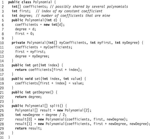
Figure 16.17 The Polynomial class.
Your task is to devise parallel addition and multiplication algorithms for this polynomial class.
1. The sum of P (x) and Q (x) can be decomposed as follows:
![]()
a) Use this decomposition to construct a task-based concurrent polynomial addition algorithm in the manner of Fig. 16.13.
b) Compute the work and critical path length of this algorithm.
2. The product of P (x) and Q (x) can be decomposed as follows:
![]()
a) Use this decomposition to construct a task-based concurrent polynomial multiplication algorithm in the manner of Fig. 16.4
b) Compute the work and critical path length of this algorithm.
Exercise 191. Give an efficient and highly parallel multithreaded algorithm for multiplying an n × n matrix A by a length-n vector x that achieves work Θ(n2) and critical path Θ(log n). Analyze the work and critical-path length of your implementation, and give the parallelism.
Exercise 192.Fig. 16.18 shows an alternate way of rebalancing two work queues: first, lock the smaller queue, then lock the larger queue, and rebalance if their difference exceeds a threshold. What is wrong with this code?

Figure 16.18 Alternate rebalancing code.
Exercise 193.
1. In the popBottom() method of Fig. 16.10, the bottom field is volatile to assure that in popBottom() the decrement at Line 15 is immediately visible. Describe a scenario that explains what could go wrong if bottom were not declared as volatile.
2. Why should we attempt to reset the bottom field to zero as early as possible in the popBottom() method? Which line is the earliest in which this reset can be done safely? Can our BoundedDEQueue overflow anyway? Describe how.
Exercise 194.
![]() In popTop(), if the compareAndSet() in Line 8 succeeds, it returns the element it read right before the successful compareAndSet() operation. Why is it important to read the element from the array before we do the compareAndSet()?
In popTop(), if the compareAndSet() in Line 8 succeeds, it returns the element it read right before the successful compareAndSet() operation. Why is it important to read the element from the array before we do the compareAndSet()?
Exercise 195. What are the linearization points of the UnboundedDEQueue methods? Justify your answers.
Exercise 196. Modify the popTop() method of the linearizable BoundedDEQueue implementation so it will return null only if there are no tasks in the queue. Notice that you may need to make its implementation blocking.
Exercise 197. Do you expect that the isEmpty() method call of a BoundedDEQueue in the executer pool code will actually improve its performance?
1 In real code, you should check that all the dimensions agree. Here we omit most safety checks for brevity.
2 In practice, it is usually more efficient to stop the recursion well before reaching a matrix size of one. The best size will be platform-dependent.
3 See Chapter 10, Pragma 10.6.1.
4 In a C or C++ implementation you would need to introduce a write barrier as described in Appendix B.