The most common difficulty that you may encounter when trying to solve SQL problems is when you have to program against what might charitably be called an “unconventional” design. Writing a query that performs well is often the most visible challenge. However, I must underline that the complex SQL queries that are forced upon developers by a poor design only mirror the complication of programs (including triggers and stored procedures) that the same poor design requires in order to perform basic operations such as integrity checking. By contrast, a sound design allows you to declare constraints and let the DBMS check them for you, removing much of the risk associated with complexity. After all, ensuring data integrity is exactly what a DBMS, a rather fine piece of software, has been engineered to achieve. Unfortunately, haphazard designs will force you to spend days coding application controls. As a bonus, you get very high odds of letting software bugs creep in. Unlike popular software systems that are in daily use by millions of users, where bugs are rapidly exposed and fixed, your home-grown software can hide bugs for weeks or months before they are discovered.

Rows That Should Have Been Columns

Rows that should have been originally specified as columns are most often encountered with that appalling “design” having the magical four attributes--entity_id, attribute_name, attribute_type, attribute_value--that are supposed to solve all schema evolution issues. Frighteningly, many supporters of this model seem to genuinely believe that it represents the ultimate sophistication in terms of normalization. You will find it under various, usually flattering, names—such as meta-design , or fact dimension with data warehouse designers.

Proponents of the magical four attributes praise the “flexibility” of this model. There is an obvious confusion of flexibility with flabbiness. Being able to add “attributes” on the fly is not flexibility; those attributes need to be retrieved and processed meaningfully. The dubious benefit of inserting rows instead of painstakingly designing the database in the first place is absolutely negligible compared to the major coding effort that is required, first, to process those new rows, and second, to insure some minimal degree of integrity and data consistency. The proper way to deal with varying numbers of attributes is to define subtypes, as explained in Chapter 1. Subtypes let you define clean referential integrity constraints—checks that you will not need to code and maintain. A database should not be a mere repository where data is dumped without any thought to its semantic integrity.

The predominant characteristic of queries against meta-design tables, as tables designed around our magical four attributes are sometimes called, is that you find the same table invoked a very high number of times in the from clause. Typically, queries will resemble something like:

select emp_last_name.entity_id        employee_id,
       emp_last_name.attribute_value  last_name,
       emp_first_name.attribute_value first_name,
       emp_job.attribute_value        job_description,
       emp_dept.attribute_value       department,
       emp_sal.attribute_value        salary
from employee_attributes emp_last_name,
     employee_attributes emp_first_name,
     employee_attributes emp_job,
     employee_attributes emp_dept,
     employee_attributes emp_sal
where emp_last_name.entity_id = emp_first_name.entity_id
  and emp_last_name.entity_id = emp_job.entity_id
  and emp_last_name.entity_id = emp_dept.entity_id
  and emp_last_name.entity_id = emp_sal.entity_id
  and emp_last_name.attribute_name = 'LASTNAME'
  and emp_first_name.attribute_name = 'FIRSTNAME'
  and emp_job.attribute_name = 'JOB'
  and emp_dept.attribute_name = 'DEPARTMENT'
  and emp_sal.attribute_sal = 'SALARY'
order by emp_last_name.attribute_value

Note how the same table is referenced five times in the from clause. The number of self-joins is usually much higher than in this simple example. Furthermore, such queries are frequently spiced up with outer joins as well.

A query with a high number of self-joins performs extremely badly on large volumes; it is clear that the only reason for the numerous conditions in the where clause is to patch all the various “attributes” together. Had the table been defined as the more logical employees(employee_id, last_name, first_name, job_description, department, salary), our query would have been as simple as:

select *
from employees
order by last_name

And the best course for executing this query is obviously a plain table scan. The multiple joins and associated index accesses of the query against employee_attributes are performance killers.

We can never succeed in making a query run as fast against a rotten design as it will run against a clean design. Any clever rewriting of a SQL query against badly designed tables will be nothing more than a wooden leg, returning only some degree of agility to a crippled query. However, we can often obtain spectacular results in comparison to the multiple joins approach by trying to achieve a single pass on the attribute table.

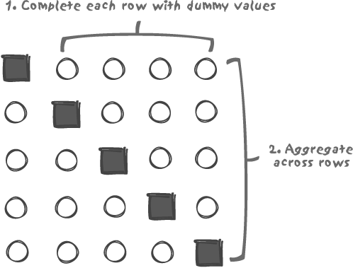
We basically want one row with several attributes (reflecting what the table design should have been in the first place) instead of multiple rows, each with only one attribute of interest per row. Consolidating a multi-row result into a single row is a feat we know how to perform: aggregate functions do precisely this. The idea is therefore to proceed in two steps, as shown in Figure 11-1:

1. Complete each row that contains only one value of interest, with as many dummy values as required to obtain the total number of attributes that we ultimately want.

2. Aggregate the different rows so as to keep only the single value of interest from each (the single value in each column). A function such as max( ), that has the advantage of being applicable to most data types, is perfect for this kind of operation.

To be certain that max( ) will only retain meaningful values, we must use dummy values that will necessarily be smaller than any legitimate value we may have in a given column. It is probably better to use an explicit value rather than null as a dummy value, even though max( ) ignores null values according to the standard.

If we apply the “recipe” illustrated in Figure 11-1 to our previous example, we can get rid of the numerous joins by writing:

Figure 11-1. Transmogrification of several rows into one row

select employee_id,
       max(last_name)        last_name,
       max(first_name)       first_name,
       max(job_description)  job_desription,
       max(department)       department,
       max(salary)           salary
from  -- select all the rows of interest, returning
      -- as many columns as we have rows, one column
      -- of interest per row and values smaller
      -- than any value of interest everywhere else
     (select entity_id                   employee_id,
             case attribute_name
               when 'LASTNAME' then attribute_value
               else ''
             end                         last_name,
             case attribute_name
               when 'FIRSTNAME' then attribute_value
               else ''
             end                         first_name,
             case attribute_name
               when 'JOB' then attribute_value
               else ''
             end                         job_description,
             case attribute_name
               when 'DEPARTMENT' then attribute_value
               else -1
             end                         department,
             case attribute_name
               when 'SALARY' then attribute_value
               else -1
             end                         salary
      from employee_attributes
      where attribute_name in ('LASTNAME',
                               'FIRSTNAME',
                               'JOB',
                               'DEPARTMENT',
                               'SALARY')) as inner
group by inner.employee_id
order by 2

The inner query is not strictly required—we could have used a series of max(case when ... end)--but the query as written makes the two steps appear more clearly.

An aggregate is not, as you might expect, the best option in terms of performance. But in the kingdom of the blind, the one-eyed man is king, and this type of query just shown usually has no trouble outperforming one having a monstrous number of self-joins. A word of caution, though: in order to accommodate any unexpectedly lengthy attribute, the attribute_value column is usually a fairly large variable-length string. As a result, the aggregation process may require a significant amount of memory, and in some extreme cases you may run into difficulties if the number of attributes exceeds a few dozen.

Important

Multiple self-joins can often be avoided by retrieving all rows in a single pass, spreading the values across separate columns, and using an aggregate function to collapse the many rows into one.

Columns That Should Have Been Rows

In contrast to the previous design in which rows have been defined for each attribute, another example of poor design occurs where columns are created instead of individual rows. The classic design mistake made by many beginners is to predefine a fixed number of columns for a number of variables, with some of the columns set to null when values are missing. A typical example is illustrated in Figure 11-2, with a very poorly designed movie database (compare this design to the correct design of Figure 8-3 in Chapter 8).

Figure 11-2. A badly designed movie database

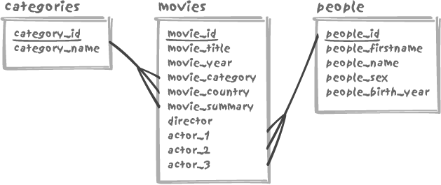
Instead of using a movie_credits table as we did in Chapter 8 to link the movies table to the people table and record the nature of each individual’s involvement, the poor design shown in Figure 11-2 assumes that we will never need to record more than a fixed number of lead actors and one director. The first assumption is blatantly wrong and so is the second one since many sketch comedies have had multiple directors. As a representation of reality, this model is plainly flawed, which should already be sufficient reason to discard it. To make matters worse, a poor design, in which data is stored as columns and yet reporting output obviously requires data to be presented as rows, often results in rather confusing queries. Unfortunately, writing queries against poor database designs seems to be as unavoidable as taxes and death in the world of SQL development.

When you want different columns to be displayed as rows, you need a pivot table. Pivot tables are used to pivot, or turn sideways, tables where we want to see columns as rows. A pivot table is, in the context of SQL databases, a utility table that contains only one column, filled with incrementing values from 1 to whatever is needed. It can be a true table or a view—or even a query embedded in the from clause of a query. Using such a utility table is a favorite old trick of experienced SQL developers, and the next few subsections show how to create and use them.

Creating a pivot table

The constructs you have seen in Chapter 7 for walking trees are usually quite convenient for generating pivot table values; for instance, we can use a recursive withaction with those database systems that support it. Here is a DB2 example to generate numbers from 1 to 50:

with pivot(row_num)
   -- Generate 50 values
   -- 1 to 50, one value per row
   as (select 1 row_num
      from sysibm.sysdummy1
      union all
      select row_num + 1
      from pivot
      where row_num < 50)
select row_num
from pivot;

Similar tricks are of course possible with Oracle’s connect by; for instance:^[*]

select level
from dual
connect by level <= 50

Using one of these constructs inside the from clause of a query can make that query particularly illegible, and it is therefore often advisable to use a regular table as pivot. But a recursive query can be useful to fill the pivot table (an alternate solution to fill a pivot table is to use Cartesian joins between existing tables). Typically, a pivot table would hold something like 1,000 rows.

Multiplying rows with a pivot table

Now that we have a pivot table, what can we do with it? One way to look at a pivot table is to view it as a row-multiplying device. By combining a pivot to a table we want to see pivoted, we repeat each of the rows of the table to be transformed as many times as we wish. Specifying the number of times we want to see one row repeated is simply a matter of adding to the join a limiting condition on the pivot table, for instance:

where pivot.row_num <= multiplying value

We can thus multiply the three rows in a test employees table in a very simple way. First, here are the three rows:

SQL> select name, job
  2  from employees;
NAME       JOB
---------- ------------------------------
Tom        Manager
Dick       Software engineer
Harry      Software engineer

And now, here is the multiplication, by three, of those rows:

SQL> select e.name, e.job, p.row_num
  2  from employees e,
  3       pivot     p
  4  where p.row_num <= 3;

NAME       JOB                               ROW_NUM
---------- ------------------------------ ----------
Tom        Manager                                 1
Dick       Software engineer                       1
Harry      Software engineer                       1
Tom        Manager                                 2
Dick       Software engineer                       2
Harry      Software engineer                       2
Tom        Manager                                 3
Dick       Software engineer                       3
Harry      Software engineer                       3

9 rows selected.

It’s best to index the only column in the pivot table so as not to fully scan this table when you need to use very few rows from it (as in the preceding example).

Using pivot table values

Besides the mere multiplying effect, the Cartesian join also allows us to associate a unique number in the range 1 to multiplying value for every copy of a row of the table we want to pivot. This value is simply the row_num column contributed by the pivot table, and it will enable us in turn to pick from each copy of a row only partial data. The full process of multiplication of the source rows and selection is illustrated, with a single row, in Figure 11-3. If we want the initial row to finally appear as a single column (which by the way implicitly requires the data types of col1 ... coln to be consistent), we must pick just one column into each of the rows generated by the Cartesian product. By checking the number coming from the pivot table, we can specify with a case for each resulting row which column is to be displayed to the exclusion of all the others. For instance, we can decide to display col1 if the value coming from the pivot table is 1, col2 if it is 2, and so on.

Figure 11-3. Pivoting a row

Needless to say, multiplying rows and discarding most of the columns we are dealing with is not the most efficient way of processing data; keep in mind that we are rowing upstream. An ideal database design would avoid the need for such multiplication and discarding.

Interestingly, and still in the hypothetical situation of a poor (to put it mildly) database design, a pivot table can in some circumstances bring direct performance benefits. Let’s suppose that, in our badly designed movie database, we want to count how many different actors are recorded (note that none of the actor_... columns are indexed, and that we therefore have to fetch the values from the table). One way to write this query is to use a union:

select count(*)
from (select actor_1
      from movies
      union
      select actor_2
      from movies
      union
      select actor_3
      from movies) as m

But we can also pivot the table to obtain something that looks more like a select on the movie_credits table of the properly designed database:

select count(distinct actor_id)
from --  Use a 3-row pivot to multiply
     --  the number of rows by 3
     --  and return actor_1 the first row in each
     --  set of 3, actor_2 for the second one
     --  and actor_3 for the third one
     (select case pv.row_num
                when 1 then actor_1
                when 2 then actor_2
                else actor_3
             end actor_id
      from movies as m,
           pivot as pv
      where pv.row_num <= 3) as m

The second version runs about twice as fast as the first one—significantly faster.

The pivot and unpivot operators

As a possibly sad acknowledgment of the generally poor quality of database designs, SQL Server 2005 has introduced two operators called pivot and unpivot to perform the toppling of rows into columns and vice-versa, respectively. The previous employee_attributes example can be written as follows using the pivot operator:

select entity_id as employee_id,
       [lastname],
       [firstname],
       [job],
       [department],
       [salary]
from employee_attributes as employees
     pivot (max(attribute_value)
            for attribute_name in ([lastname],
                                   [firstname],
                                   [job],
                                   [department],
                                   [salary])
                 as pivoted_employees
order by 2

The specific values in the attribute_name column that we want to appear as columns are listed in the for ... in clause, using a particular syntax that transforms the character data into column identifiers. There is an implicit group by applied to all the columns from employee_attributes that are not referenced in the pivot clause; we must be careful if we have other columns (for instance, an attribute_type column) than entity_id, as they may require an additional aggregation layer.

The unpivot operator performs the reverse operation, and allows us to see the link between movie and actor as a more logical collection of (movie_id, actor_id) pairs by writing:

select movie_id, actor_type, actor_id
from movies
     unpivot (actor_id for actor_type in ([actor_1],
                                          [actor_2],
                                          [actor_3])) as movie_actors

Note that this query doesn’t exactly produce the result we want, since it introduces the name of the original column as a virtual actor_type column. There is no need to qualify actors as actor_1, actor_2, or actor_3, and once again the query may need to be wrapped into another query that only returns movie_id and actor_id.

The use of a pivot table, or of the pivot and unpivot operators, is a very interesting technique that can help extricate us from more than one quagmire. The support for pivoting operators by major database systems is not, of course, to be interpreted as an endorsement of bad design, but as an example of realpolitik.

Important

Pivot tables and operators can be a useful technique in their own right, but they should never be used as a means of glossing over the inadequacies of a bad design.

Single Columns That Should Have Been Something Else

Some designers of our movie database may well have been sensitive to the limitation on the number of actors we may associate with one movie. Trying to solve design issues with a creative use of irrelevant techniques, someone may have come up with a “bright idea”: what about storing the actor identifiers as a comma-separated string in one wide actors column? For instance:

first actor id, second actor id, ...

And so much for the first normal form.... The big design mistake here is to store several pieces of data that we need to handle one by one into one column. There would be no issue if a complex string—for instance a lengthy XML message—were considered as an opaque object by the DBMS and handled as if it were an atomic item. But that’s not the case here. Here we have several values in one column, and we do want to treat and manipulate each value individually. We are in trouble.

There are only two workable solutions with a creative design of this sort:

• Scrapping it and rewriting everything. This is, of course, by far the best solution.

• When delays, costs, and politics require a fast solution, the only way out may be to apply a creative SQL solution; once again, let me state that “solution” is probably not the best choice of words in this case, “fix” would be a better description.

I’ll also point out that a more elaborate version of the same mistake could use an “XML type” column; I am going to use simple character-string manipulation functions in my example, but they could as well be XML-extracting functions.

Note

Be warned: “creative SQL” is often a euphemism for ugly SQL!

First normal form on the fly

Our problem is to extract various individual components from a string of characters and return them one by one on separate rows. This is easier with some database systems (for instance, Oracle has a very rich set of string functions that noticeably eases the work) than with others. Conventions such as systematically starting or ending the string with a comma may further help us. We are not wimps, but real SQL developers, and we are therefore going to take the north face route and assume the worst:

1. First, let’s assume that our lists of identifiers are in the following form:

   id1, id2, id3, ..., idn

2. Second, we shall also assume that the only sets of functions at our disposal are those common to the major database systems. We shall use Transact-SQL for our example and only use built-in functions. As you will see, a well-designed user function might ease both the writing and the performance of the resulting query.

Let’s start with a (very small) movies table in which a list of actor identifiers is (wrongly) stored as an attribute of the movie:

1> select movie_id, actors
2> from movies
3> go
 movie_id              actors
 --------------------- ----------------------------------------
                     1 123,456,78,96
                     2 23,67,97
                     3 67,456

(3 rows affected)

The first step is to use as many rows from our pivot table as we may have characters in the actors string—arbitrarily set to a maximum length of 50 characters. We are going to multiply the number of rows in the movies table by this number, 50. We would naturally be rather reluctant to do something similar on millions of rows (as an aside, a function allowing us to return the position of the nth separator or the nth item in the string would make it necessary to multiply only by the maximum number of identifiers we can encounter, instead of by the maximum string length).

Our next move is to use the substring( ) function to successively get subsets (that can be null) of actors, starting at the first character, then moving to the second, and so forth, up to the last character (at most, the 50th character). We just have to use the row_num value from the pivot table to find the starting character of each substring. If we take for instance the string from the actors column that is associated to the movie identified by the value 1 for movie_id, we shall get something like:

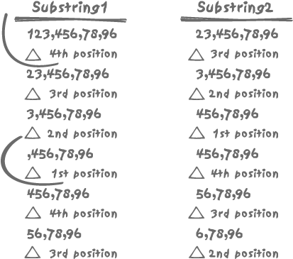
123,456,78,96  associated to the row_num value 1
23,456,78,96   associated to the row_num value 2
3,456,78,96    associated to the row_num value 3
,456,78,96      ....
456,78,96
56,78,96
6,78,96
,78,96
78,96
....

We’ll compute these subsets in a column that we’ll call substring1. Having these successive substrings, we can now check the position of the first comma in them. Our next move is to return as a column called substring2 the content of substring1 shifted by one position. We also locate the position of the first comma in substring2. These operations are illustrated in Figure 11-4. Among the various resulting rows, the only ones to be of interest are those marking the beginning of a new identifier in the string: the first row in the series that is associated with the row_num value of 1, and all the rows for which we find a comma in first position of substring1. For all these rows, the position of the comma in substring2 tells us the length of the identifier that we are trying to isolate.

Figure 11-4. Splitting-up a comma separated list

Translated into SQL code, here is what we get:

1> select row_num,
2>        movie_id,
3>        actors,
4>        first_sep,
5>        next_sep
6> from (select row_num,
7>              movie_id,
8>              actors,
9>              charindex(',', substring(actors, row_num,
10>                                      char_length(actors))) first_sep,
11>             charindex(',', substring(actors, row_num + 1,
12>                                  char_length(actors))) + 1 next_sep
13>      from movies,
14>           pivot
15>     where row_num <= 50) as q
16> where row_num = 1
17>    or first_sep = 1
18> go
 row_num     movie_id       actors             first_sep   next_sep
 ----------- -------------- ------------------ ----------- -----------
           1              1 123,456,78,96                4           4
           4              1 123,456,78,96                1           5
           8              1 123,456,78,96                1           4
          11              1 123,456,78,96                1           1
           1              2 23,67,97                     3           3
           3              2 23,67,97                     1           4
           6              2 23,67,97                     1           1
           1              3 67,456                       3           3
           3              3 67,456                       1           1

(9 rows affected)

If we accept that we must take some care to remove commas, and the particular cases of both the first and last identifiers in a list, getting the various identifiers is then reasonably straightforward, even if the resulting code is not for the faint-hearted:

1> select movie_id,
2>        actors,
3>        substring(actors,
4>                  case row_num
5>                    when 1 then 1
6>                    else row_num + 1
7>                  end,
8>                  case next_sep
9>                    when 1 then char_length(actors)
10>                   else
11>                     case row_num
12>                       when 1 then next_sep - 1
13>                       else next_sep - 2
14>                     end
15>                 end) as id
16> from (select row_num,
17>              movie_id,
18>              actors,
19>              first_sep,
20>              next_sep
21>       from (select row_num,
22>                    movie_id,
23>                    actors,
24>                    charindex(',', substring(actors, row_num,
25>                              char_length(actors))) first_sep,
26>                    charindex(',', substring(actors, row_num + 1,
27>                              char_length(actors))) + 1 next_sep
28>             from movies,
29>                  pivot
30>             where row_num <= 50) as q
31>       where row_num = 1
32>          or first_sep = 1) as q2
33> go
 movie_id         actors                         id
 ---------------- ------------------------------ -----------------
                1 123,456,78,96                  123
                1 123,456,78,96                  456
                1 123,456,78,96                  78
                1 123,456,78,96                  96
                2 23,67,97                       23
                2 23,67,97                       67
                2 23,67,97                       97
                3 67,456                         67
                3 67,456                         456

(9 rows affected)

We could have made the code slightly simpler by prepending and appending a comma to the actors column. I leave doing that as an exercise for the undaunted reader. Note that as the left alignment shows, the resulting id column is a string and should be explicitly converted to numeric before joining to the table that stores the actors’ names.

The preceding case, besides being an interesting example of solving a SQL problem by successively wrapping queries, also comes as a healthy warning of what awaits us on the SQL side of things when tables are poorly designed.

Lifting the veil on the Chapter 7 mystery path explosion

You may remember that in Chapter 7 I described the materialized path model for tree representations. In that chapter I noted that it would be extremely convenient if we could “explode” a materialized path into the different materialized paths of all its ancestors. The advantage of this method is that when we want to walk a hierarchy from the bottom up, we can make efficient use of the index that should hopefully exist on the materialized path. If we don’t “explode” the materialized path, the only way we have to find the ancestors of a given row is to specify a condition such as:

and offspring.materialized_path
    like concat(ancestor.materialized_path, '%')

Sadly, this is a construct that cannot use the index (for reasons that are quite similar to those in the credit card prefix problem of Chapter 8).

How can we “explode” the materialized path? The time has come to explain how we can pull that rabbit out of the hat. Since our node will have, in the general case, several ancestors, the very first thing we have to do is to multiply the rows by the number of preceding generations. In this way we’ll be able to extract from the materialized path of our initial row (for example the row that represents the Hussar regiment under the command of Colonel de Marbot) the paths of the various ancestors. As always, the solution for multiplying rows is to use a pivot table. If we do it this time with MySQL, there is a function called substring_index( ) that very conveniently returns the substring of its first argument from the beginning up to the third argument occurrence of the second argument (hopefully, the example is easier to understand). To know how many rows we need from the pivot table, we just compute how many elements we have in the path in exactly the same way that we computed the depth in Chapter 7, namely by comparing the length of the path to the length of the same when separators have been stripped off. Here is the query, and the results:

mysql>  select mp.materialized_path,
    ->         substring_index( mp.materialized_path, '.', p.row_num )
    ->                                     as ancestor_path
    -> from materialized_path_model as mp,
    ->      pivot as p
    -> where mp.commander = 'Colonel de Marbot'
    ->   and p.row_num <= 1 + length( mp.materialized_path )
    ->                      - length(replace(mp.materialized_path, '.', ''));
+-------------------+---------------+
| materialized_path | ancestor_path |
+-------------------+---------------+
| F.1.5.1.1         | F             |
| F.1.5.1.1         | F.1           |
| F.1.5.1.1         | F.1.5         |
| F.1.5.1.1         | F.1.5.1       |
| F.1.5.1.1         | F.1.5.1.1     |
+-------------------+---------------+
5 rows in set (0.00 sec)

There is another, and rather important, use of pivot tables that I must now mention. In previous chapters I have underlined the importance of binding variables , in other words of passing parameters to SQL queries. Variable binding allows the DBMS kernel to skip the parsing phase (in other words, the compilation of the statement) after it has done it once. Keep in mind that parsing includes steps as potentially costly as the search for the best execution path. Even when SQL statements are dynamically constructed, it is quite possible, as you have seen in Chapter 8, to pass variables to them. There is, however, one difficult case: when the end user can make multiple choices out of a combo box and pass a variable number of parameters for use in an in list. The selection of multiple values raises several issues:

The ability provided by pivot tables to split a string allows us to pass a list of values as a single string to the statement, irrespective of the actual number of values. This is what I am going to demonstrate with Oracle in this section.

The following example shows how most developers would approach the problem of passing a list of values to an in list when that list of values is contained within a single string. In our case the string is v_list, and most developers would concatenate several strings together, including v_list, to produce a complete select statement:

v_statement := 'select count(order_id)'
                   || ' from order_detail'
                   || ' where article_id in ('
                   || v_list || ')';
execute immediate v_statement into n_count;

This example looks dynamic, but for the DBMS it’s in fact all hardcoded. Two successive executions will each be different statements, both of which will have to be parsed before execution. Can we pass v_list as a parameter to the statement, instead of concatenating it into the statement? We can, by applying exactly the same techniques to the comma-separated value stored in variable v_list as we have applied to the comma-separated value stored in column actors in the example of on-the-fly normalization. A pivot table allows us to write the following somewhat wilder SQL statement:

select count(od.order_id)
into n_count
from order_detail od,
     (  -- Return at many rows as we have items in the list
        -- and use character functions to return the nth item
        -- on the nth row
      select to_number(substr(v_list,
                              case row_num
                                when 1 then 1
                                else 1 + instr(v_list, ',', 1, row_num - 1)
                               end,
                               case instr(v_list, ',', 1, row_num)
                                 when 0 then length(v_list)
                                 else
                                   case row_num
                                     when 1  then instr(v_list, ',',
                                                        1, row_num) - 1
                                     else instr(v_list, ',', 1, row_num) - 1
                                          - instr(v_list, ',',
                                                  1, row_num - 1)
                                   end
                                 end)) article_id
      from pivot
      where instr(v_list||',', ',', 1, row_num) > 0
        and row_num <= 250) x
where od.article_id = x.article_id;

You may need, if you are really motivated, to study this query a bit to figure out how it all works. The mechanism is all based on repeated use of the Oracle function instr( ). Let me just say that this function instr( haystack , needle , from_pos , count ) returns the countth occurrence of needle in haystack starting at position from_pos (0 is returned when nothing is found), but the logic is exactly the same as with the previous examples.

I have run the pivot and hardcoded versions of the query successively 1, 10, 100, 1,000, 10,000, and 100,000 times. Each time, I randomly generated a list of from 1 to 250 v_list values. The results are shown in Figure 11-5, and they are telling: the “pivoted” list is 30% faster as soon as the query is repeatedly executed.

Figure 11-5. Performance of a hardcoded list versus a list transformed with a pivot table

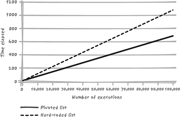
Remember that the execution of a hardcoded query requires parsing and then execution, while a query that takes parameters (bind variables) can be re-executed subsequently for only a marginal cost of the first execution. Even if this later query is noticeably more complicated, as long as the execution is faster than execution plus parsing for the hardcoded query, the later query wins hands-down in terms of performance.

There are actually two other benefits that don’t show up in Figure 11-5:

Some people have trouble writing SQL queries that return aggregates for bands. Such queries are actually quite easy to write using the case construct. By way of example, look at the problem of reporting on the distribution of tables by their total row counts. For instance, how many tables contain fewer than 100 rows, how many contain 100 to 10,000 rows, how many 10,000 to 1,000,000 rows, and how many tables store more than 1,000,000 rows?

Information about tables is usually accessible through data dictionary views: for instance, INFORMATION_SCHEMA.TABLES, pg_statistic, and pg_tables, dba_tables, syscat.tables, sysobjects and systabstats, and so on. In my explanation here, I’ll assume the general case of a view named table_info, containing, among other things, the columns table_name and row_count. Using this table, a simple use of case and the suitable group by can give us the distribution by row_count that we are after:

select case
         when row_count < 100
              then 'Under 100 rows'
          when row_count >= 100 and row_count < 10000
               then '100 to 10000'
          when row_count >= 10000 and row_count < 1000000
               then '10000 to 1000000'
          else
               'Over 1000000 rows'
        end as range,
        count(*) as table_count
from table_info
where row_count is not null
group by case
           when row_count < 100
                then 'Under 100 rows'
           when row_count >= 100 and row_count < 10000
                then '100 to 10000'
           when row_count >= 10000 and row_count < 1000000
                then '10000 to 1000000'
           else
                'Over 1000000 rows'
         end

There is only one snag here: group by performs a sort before aggregating data. Since we are associating a label with each of our aggregates, the result is, by default, alphabetically sorted on that label:

RANGE             TABLE_COUNT
----------------- ------------
100 to 10000                18
10000 to 1000000            15
Over 1000000 rows            6
Under 100 rows              24

The ordering that would be logical to a human eye in such a case is to see Under 100 rows appear first, and then each band by increasing number of rows, with Over 1,000,000 rows coming last. Rather than trying to be creative with labels, the stratagem to solve this problem consists of two steps:

Here is the query that results from applying the preceding two steps:

select row_range, table_count
from ( -- Build a sort key to have bands suitably ordered
       -- and hide it inside a subquery
       select case
               when row_count < 100
                 then 1
               when row_count >= 100 and row_count < 10000
                 then 2
               when row_count >= 10000 and row_count < 1000000
                 then 3
               else
                 4
             end as sortkey,
             case
               when row_count < 100
                 then 'Under 100 rows'
               when row_count >= 100 and row_count < 10000
                 then '100 to 10000'
               when row_count >= 10000 and row_count < 1000000
                 then '10000 to 1000000'
               else
                 'Over 1000000 rows'
             end  as row_range,
             count(*) as table_count
      from table_info
      where row_count is not null
      group by case
                 when row_count < 100
                   then 'Under 100 rows'
                 when row_count >= 100 and row_count < 10000
                   then '100 to 10000'
                 when row_count >= 10000 and row_count < 1000000
                   then '10000 to 1000000'
                 else
                   'Over 1000000 rows'
               end,
               case
                 when row_count < 100
                   then 1
                 when row_count >= 100 and row_count < 10000
                   then 2
                 when row_count >= 10000 and row_count < 1000000
                   then 3
                 else
                   4
               end) dummy
order by sortkey;

And following are the results from executing that query:

ROW_RANGE         TABLE_COUNT
----------------- -----------
Under 100 rows             24
100 to 10000               18
10000 to 1000000           15
Over 1000000 rows           6

The technique of hiding a sort key within a query in the from clause, which I used in the previous section to display bands, can also be helpful in other situations. A particularly important case is when a table contains the definition of a general rule that happens to be superseded from time to time by a particular case defined in another table. I’ll illustrate by example.

I mentioned in Chapter 1 that the handling of various addresses is a difficult issue. Let’s take the case of an online retailer, one that knows at most two addresses for each customer: a billing address and a shipping address. In most cases, the two addresses are the same. The retailer has decided to store the mandatory billing address in the customers table and to associate the customer_id identifier with the various components of the address (line_1, line_2, city, state, postal_code, country) in a different shipping_addresses table for those few customers for whom the two addresses differ.

The wrong way to get the shipping address when you know the customer identifier is to execute two queries:

An alternate way to approach this problem is to apply an outer join on shipping_addresses and customers. You will then get two addresses, one of which will in most cases be a suite of null values. Either you check programmatically if you indeed have a valid shipping address, which is a bad solution, or you might imagine using the coalesce( ) function that returns its first non-null argument:

select ... coalesce(shipping_address.line_1, customers.line_1), ...

Such a use of coalesce( ) would be a very dangerous idea, because it implicitly assumes that all addresses have exactly the same number of non-null components. If you suppose that you do indeed have a different shipping address, but that its line_2 component is null while the line_2 component of the billing address is not, you may end up with a resulting invalid address that borrows components from both the shipping and billing addresses. A correct approach is to use case to check for a mandatory component from the address—which admittedly can result in a somewhat difficult to read query. An even better solution is probably to use the “hidden sort key” technique, combined with a limit on the number of rows returned (select top 1..., limit 1, where rownum = 1 or similar, depending on the DBMS) and write the query as follows:

select *
from (select 1 as sortkey,
             line_1,
             line_2,
             city,
             state,
             postal_code,
             country
      from shipping_addresses
      where customer_id = ?
      union
      select 2 as sortkey,
             line_1,
             line_2,
             city,
             state,
             postal_code,
             country
      from customers
      where customer_id = ?
      order by 1) actual_shipping_address
limit 1

The basic idea is to use the sort key as a preference indicator. The limit set on the number of rows returned will therefore ensure that we’ll always get the “best match” (note that similar ideas can be applied to several rows when a row_number( ) OLAP function is available). This approach greatly simplifies processing on the application program side, since what is retrieved from the DBMS is “certified correct” data.

The technique I’ve just described can also be used in multilanguage applications where not everything has been translated into all languages. When you need to fetch a message, you can define a default language and be assured that you will always get at least some message, thus removing the need for additional coding on the application side.

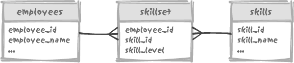
An interesting problem is that of how to write queries based on some criteria referring to a varying list of values. This case is best illustrated by looking for employees who have certain skills, using the three tables shown in Figure 11-6. The skillset table links employees to skills, associating a 1 to 3 skill_level value to distinguish between honest competency, strong experience, and outright wizardry.

Figure 11-6. Tables used for querying employee skills

Finding employees that have a level 2 or 3 SQL skill is easy enough:

select e.employee_name
from employees e
where e.employee_id in
     (select ss.employee_id
      from skillset ss,
           skills s
      where s.skill_id = ss.skill_id
        and s.skill_name = 'SQL'
        and ss.skill_level >= 2)
order by e.employee_name

(We can also write the preceding query with a simple join.) If we want to retrieve the employees who are competent with Oracle or DB2, all we need to do is write:

select e.employee_name, s.skill_name, ss.skill_level
from employees e,
     skillset ss,
     skills s
where e.employee_id = ss.employee_id
  and s.skill_id = ss.skill_id
  and s.skill_name in ('ORACLE', 'DB2')
order by e.employee_name

No need to test for the skill level, since we will accept any level. However, we do need to display the skill name; otherwise, we won’t be able to tell why a particular employee was returned by the query. We also encounter a first difficulty, namely that people who are competent in both Oracle and DB2 will appear twice. What we can try to do is to aggregate skills by employee. Unfortunately, not all SQL dialects provide an aggregate function for concatenating strings (you can sometimes write it as a user-defined aggregate function, though). We can nevertheless perform a skill aggregate by using the simple stratagem of a double conversion . First we convert our value from string to number, then from number back to string once we have aggregated numbers.

Skill levels are in the 1 through 3 range. We can therefore confidently represent any combination of Oracle and DB2 skills by a two-digit number, assigning for instance the first digit to DB2 and the second one to Oracle. This is easily done as follows:

select e.employee_name,
       (case s.skill_name
          when 'DB2' then 10
          else 1
        end) * ss.skill_level as computed_skill_level
from employees e,
     skillset ss,
     skills s
where e.employee_id = ss.employee_id
  and s.skill_id = ss.skill_id
  and s.skill_name in ('ORACLE', 'DB2')

computed_skill_level will result in 10, 20, or 30 for DB2 skill levels, while Oracle skill levels will remain 1, 2, and 3. We then can very easily aggregate our skill levels, and convert them back to a more friendly description:

select employee_name,
       --  Decode the numerically encoded skill + skill level combination
       --  Tens are DB2 skill levels, and units Oracle skill levels
      case
        when aggr_skill_level >= 10
          then 'DB2:' + str(round(aggr_skill_level/10,0)) + ' '
      end
      + case
          when aggr_skill_level % 10 > 0
           then 'Oracle:' + str(aggr_skill_level % 10)
       end as skills
from (select e.employee_name,
             -- Numerically encode skill + skill level
             -- so that we can aggregate them
             sum((case s.skill_name
                    when 'DB2' then 10
                    else 1
                  end) * ss.skill_level)  as aggr_skill_level
      from employees e,
           skillset ss,
           skills s
      where e.employee_id = ss.employee_id
        and s.skill_id = ss.skill_id
        and s.skill_name in ('ORACLE', 'DB2')
     group by e.employee_name) as encoded_skills
order by employee_name

But now let’s try to answer a more difficult question. Suppose that the project we want to staff happens to be a migration from one DBMS to another one. Instead of finding people who know Oracle or DB2, we want people who know both Oracle and DB2.

We have several ways to answer such a question. If the SQL dialect we are using supports it, the intersect operator is one solution: we find people who are skilled on Oracle on one hand, people who are skilled on DB2 on the other hand, and keep the happy few that belong to both sets. We certainly can also write the very same query with an in( ):

select e.employee_name
from employees e,
     skillset ss,
     skills s
where s.skill_name = 'ORACLE'
  and s.skill_id = ss.skill_id
  and ss.employee_id = e.employee_id
  and e.employee_id in (select ss2.employee_id
                        from skillset ss2,
                             skills s2
                        where s2.skill_name = 'DB2'
                          and s2.skill_id = ss2.skill_id)

We can also use the double conversion solution and filter on the numerical aggregate by using the same expressions as we have been using for decoding the encoded_skills computed column. The double conversion stratagem has other advantages:

Let’s conclude our adventures in the SQL wilderness by combining several of the techniques shown in this chapter and try to select employees on the basis of some rather complex and fuzzy conditions. We want to find, from among our employees, that one member of staff who happens to be the best candidate for a project that requires a range of skills across several different environments (for example, Java, .NET, PHP, and SQL Server). The ideal candidate is a guru in all environments; but if we issue a query asking for the highest skill level everywhere it shall probably return no row. In the absence of the ideal candidate, we are usually left with imperfect candidates, and we must identify someone who has the best competency in as many of our environments as possible and is therefore the best suited for the project. For instance, if our Java guru is a world expert, but knows nothing of PHP, that person is unlikely to be selected.

“Best suited” implies a comparison between the various employees, or, in other words, a sort, from which the winner will emerge. Since we want only one winner, we shall have to limit the output of our list of candidates to the first row. You should already be beginning to see the query as a select ... from (select ... order by) limit 1 or whatever your SQL dialect permits.

The big question is, of course, how we are going to order the employees. Who is going to get the preference between one who has a decent knowledge of three of the specified topics, and one who is an acknowledged guru of two subjects? It is likely, in a case such as we are discussing, that the width of knowledge is what matters more to us than the depth of knowledge. We can use a major sort key on the number of skills from the requirement list that are mastered, and a minor sort key on the sum of the various skill_level values by employee for the skills in the requirement list. Our inner query comes quite naturally:

select e.employee_name,
       count(ss.skill_id) as major_key,
       sum(ss.skill_level) as minor_key
from employees e,
     skillset ss,
     skills s
where s.skill_name in ('JAVA', '.NET', 'PHP', 'SQL SERVER')
  and s.skill_id = ss.skill_id
  and ss.employee_id = e.employee_id
group by e.employee_name
order by 2, 3

This query, however, doesn’t tell us anything about the actual skill level of our best candidate. We should therefore combine this query with a double conversion to get an encoding of skills. I leave doing that as an exercise, assuming that you have not yet reached a semi-comatose state.

You should also note, from a performance standpoint, that we need not refer to the employees table in the inner query. The employee name is information that we need only when we display the final result. We should therefore handle only employee_id values, and do the bulk of the processing using the tables skills and skillset. You should also think about the rare situation in which two candidates have exactly the same skills—do you really want to restrict output to one row?

I shall conclude this chapter with a cautionary note about optimizer directives . An SQL optimizer can be compared to the program that computes shutter speed and exposure in an automated camera. There are conditions when the “auto” mode is no longer appropriate—for instance, when the subject of the picture is backlit or for the shooting of night scenes. Similarly, all database systems provide one way or another to override or at least direct decisions taken by the query optimizer in its quest for the Dream Execution Path. There are basically two techniques to constrain the optimizer:

In the latter case the syntax between products varies, since you may have these directives written as an inherent part of the SQL statement (for instance force index(...) with MySQL or option loop join with Transact-SQL), or written as a special syntax comment (such as /*+ all_rows */ with Oracle).

Optimizer directives have so far been mostly absent from this book, and for good reasons. Repeatedly executing queries against living data is, to some degree, similar to repeatedly photographing the same subject at various times of day: what is backlit in the morning may be in full light in the afternoon. Directives are destined to override particular quirks in the behavior of the optimizer and are better left alone. The most admissible directives are those directives specifying either the expected outcome, such as sql_small_result or sql_big_result with MySQL, or whether we are more interested in a fast answer, as is generally the case in transactional processing, with directives such as option fast 100 with SQL Server or /*+ first_rows(100) */ with Oracle. These directives, which we could compare to the “landscape” or “sports” mode of a camera, provide the optimizer with information that it would not otherwise be able to gather. They are directives that don’t depend on the volume or distribution of data; they are therefore stable in time, and they do add value. In any case, even directives that add value should not be employed unless they are required. The optimizer is able to determine a great deal about the best way to proceed when it is given a properly written query in the first place. The best and most simple example of implicit guidance of the optimizer is possibly the use of correlated versus uncorrelated subqueries. They are to be used under dissimilar circumstances to achieve functionally identical results.

One of the nicest features of database optimizers is their ability to adapt to changing circumstances. Freezing their behavior by using constraining directives is indicative of a very short-term view that can be potentially damaging to performance in the future. Some directives are real time-bombs, such as those specifying indexes by name. If, for one reason or another a DBA renames an index used in a directive, the result can be disastrous. We can get a similarly catastrophic effect when a directive specifies a composite index, and this index is rebuilt one day with a different column order.

Let me add that it is common to see inexperienced developers trying to derive a query from an existing one. When the original query contains directives, beginners rarely bother to question whether these directives are appropriate to their new case. Beginners simply apply what they see as minor changes to the select list and the search criteria. As a result, you end up with queries that look like they have been fine-tuned, but that often follow a totally irrelevant execution path.